Electron Correlations in Bilayer Graphene
Abstract
The nature of electron correlations in bilayer graphene has been investigated. An analytic expression for the radial distribution function is derived for an ideal electron gas and the corresponding static structure factor is evaluated. We also estimate the interaction energy of this system. In particular, the functional form of the pair-correlation function was found to be almost insensitive to the electron density in the experimentally accessible range. The inter-layer bias potential also has a negligible effect on the pair-correlation function. Our results offer valuable insights into the general behavior of the correlated systems and serve as an essential starting-point for investigation of the fully-interacting system.
pacs
73.22.Pr, 71.10.-wDespite intense studies for many decades, the important role of many-particle correlations in electron liquids [1], particularly in systems with reduced dimensions, remains a challenging issue in condensed-matter physics. This subject has become even more pressing in recent years as the physical properties of graphene have been unmasked at a rapid pace [2]. Monolayer and bilayer graphene are totally new classes of two-dimensional electron systems with unusual band structures and chiral charge carriers. The influence of electron correlations on various physical properties of the chiral two-dimensional electron gas in monolayer graphene has been the subject of several investigations [3, 4, 5]. These were all carried out with the aid of established pertubative techniques. On the other hand, our earlier work based on exact analytical treatment [6] indicated that the electron correlations completely vanish from the two-particle kinetic energy of monolayer graphene, a fact which was attributed to the specific spinor structure of the single-particle wave functions which in turn is a direct manifestation of the chirality of the massless Dirac fermions in monolayer graphene. Such cancellations were not found to occur for electrons in bilayer graphene [6], due to the massive chiral nature of the low-energy quasiparticles. Clearly, we have a long way to go in order to find a satisfactory understanding of the role interactions play in these unique electron systems, but it is evident that the effects of correlations in bilayer graphene is an important and relevant issue.
In this Rapid Communication, we will lay out the foundation for the process of establishing the behavior of the correlation function of interacting electrons in bilayer graphene, which is an essential step for evaluation of the thermodynamic properties of this system. We derive an analytic expression for the pair-correlation function (PCF) of an ideal electron system, and use it to compute the corresponding static structure factor as a function of the electron density. We make a detailed comparison of the PCF with the same quantity in a traditional two-dimensional electron gas (2DEG), and compute the exchange energy for the bilayer graphene system. Evaluation of the PCF with full electron correlations included is certainly a very arduous task [7], and has not yet been attempted for bilayer graphene. Our present approach is an important and necessary first step in describing a fully correlated system, but it already provides valuable insights into the general behavior of these functions.
Bilayer graphene has a hexagonal Brillouin zone where the low-energy features are located near two inequivalent corners, called the K points [8, 9]. There are four low-energy bands for each spin species in the vicinity of each K point. In unbiased bilayer graphene the second and third of these bands (called the ‘low-energy branches’) touch exactly at the charge-neutrality point, making intrinsic bilayer graphene a zero-gap semiconductor. There are two more bands (the ‘split’ branches), each seperated from the low-energy branch by the inter-layer coupling parameter . We label these bands as follows: The conduction and valence bands are given by ; the branches are ; the valleys are ; and the spins are . Adding the electron wave vector , we have the complete set of quantum numbers . At half-filling, all eight valence bands are filled, and the eight conduction bands are empty.
Spin- and valley-dependent contributions to the PCF are defined as [1]
| (1) |
where is the field operator for an electron in valley with spin . The total PCF can be expressed in terms of these functions as .
To evaluate this expression we substitute the well-known form of the single-particle wave functions in bilayer graphene
| (2) |
where and are respectively the valley and spin parts of the wave function, is the normalization area, and the functional form of the wave function components and single-particle energies are easily derived from the Schrödinger equation for the tight-binding Hamiltonian. Substituting Eq. (2) into Eq. (1), we find that
| (3) |
with and where is the occupancy of state . As expected, the off-diagonal components of the PCF are constant with unit value. We have also assumed that (i.e. that electrons are equally distributed between the valley and spin components and that electron density is uniform in space).
To procede, we must be careful about how we define the various densities. The total density of electrons is denoted by , but we also consider the density of charge carriers (also called the excess density) which may be either positive (for electrons) or negative (for holes). Then, the sums over occupied wave vector states must be taken independently for each combination of band and branch quantum numbers. Taking the limit of an infinite system (with the electron density held constant) means that we can replace the sums over wave vectors with two-dimensional integrals. The integrals which result from this procedure are not automatically convergent for large wave vectors. Therefore, we must introduce a cut-off wave vector using some physical reasoning. Consideration of the lattice structure shows that each unit cell contributes four electrons (one per carbon atom), so that the density of electrons at half-filling is where is the lattice constant. Therefore, we can set the wave vector cut-off because
where is the total number of electrons at half-filling. As an example, in intrinsic graphene (where the Fermi energy is exactly at the charge neutrality point) the valence bands are all filled and the conduction bands are all empty. Therefore, the sum over bands and branches in Eq. (3) becomes
Using the expressions for the wave functions in Eq. (2) and evaluating the elementary integrations over the angles, we arrive at
| (4) |
where all terms are evaluated with , and and are the zeroeth order and first order cylindrical Bessel function respectively. In the case of positively-doped graphene (where the charge carriers are holes and the Fermi energy is in the valence band), we assume that for moderate densities only the low-energy band is depopulated [10] so that the lower integration limit becomes the Fermi wave vector when . For negatively-doped graphene, each squared term in Eq. (4) gains a contribution from the low-energy conduction band (, ) with the Fermi wave vector replacing as the upper limit in this integral.
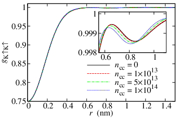
In order to obtain the PCF, these integrals are evaluated numerically and the resulting function is plotted in Fig. 1 for various densities. The behavior of the function is clearly similar to that in a conventional 2DEG [11], with an exchange hole with radius approximately . The reason that is finite is explained as follows: The PCF evaluated here specifies all-but-two quantum numbers. Therefore for any given combination of band and branch, there can be an electron at with one of three other combinations which does not violate the Pauli principle. Hence the minimum value of the PCF is , as seen in Fig 1. If we were to calculate the for a fully-specified combination of valley, spin, band and branch then this function would indeed go to zero at the origin, just as it does for the conventional 2DEG.
The dependence of the PCF on the density is tiny for physically reasonable values of the excess density. The reason for this tiny variation is that the electrons in the filled valence bands contribute more to the sum over states than those in the partially filled conduction band. The PCF contains essentially an average over all particles (where is the total number of electrons and runs over all filled states). The intrinsic density of electrons due to the valence bands which are filled in the charge-neutral case is , which is much greater than the density of charge carriers due to the excess density induced by gating or doping. Therefore when the average over all states is taken, the effect of the partially filled conduction band (or partially empty valence band) is swamped by the contribution from the filled valence band. This effect is highlighted by comparison with the non-interacting PCF in a traditional semiconductor 2DEG (in the lower inset to Fig. 1). When the 2DEG PCF is plotted for , the exchange hole is much larger than in graphene. But when the total density is used the exchange hole is of a much more similar size.
Once we obtain the radial distribution function, the static structure factor for the system can be derived from the following expression [1]
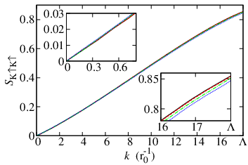
which is, in principle, an experimentally observable function via X-ray and neutron diffraction where the correlation functions are usually extracted from the measured diffraction intensity profile [12]. We have evaluated the integral numerically and the resulting function is plotted in Fig. 2 for several values of the electron density. We see that the variation with density is rather small, but at low wave vector, increases with density (upper-left inset) while at high wave vector the opposite is true (lower-right inset). The structure factor is almost linear even up to the wave vector cut-off . This behavior has been noticed before in the context of monolayer graphene [3, 7]. This is noticably different from the result for the conventional 2DEG [11], where the static structure function is roughly linear at small wave vector but saturates at for . We emphasize that the static structure function of bilayer graphene behaves similarly to the conventional 2DEG at small wave vector, but like monolayer graphene at large wave vector. This behavior might be expected when the quadratic-to-linear crossover in the hyperbolic band structure is considered.
Finally, we calculate the exchange energy per electron associated with the exchange-correlation hole
where is the Coulomb potential and we use the full . This function is linear in the quasi-particle density, with eV.
Let us now turn our attention to the effect of a finite inter-layer bias potential on the radial distribution function. When an electrostatic potential is applied perpendicularly to the plane of the graphene, a gap opens at the charge-neutrality point, and the shape of the low-energy bands changes to a ‘Mexican hat’ form [9]. This also changes the form of the wave functions, and causes the Fermi surface to become ring-shaped for small charge carrier density [13]. Therefore, the integration limits in Eq. (4) change if the Fermi energy . In that case, integrals relating to partially-filled bands become with
On the other hand, if [which occurs when ] then as before.

We plot the change in the PCF with the introduction of a bias as a function of the inter-particle separation in Fig. 3. We see that the change is greatest at small charge carrier density and large . However, overall the change is very small which is predictable since the PCF is related to the electron wave functions, and the inter-layer potential only induces a change for . Similarly, the static structure factor shows only very small deviation from the results for finite .
In conclusion, we have investigated the PCF and the corresponding static structure function for an ideal gas of electrons in bilayer graphene and compared it to the same quantity in the traditional 2DEG system. We have found behavior quite similar to that of the conventional 2DEG at equivalent density, in that an exchange hole is formed with density-dependent radius. However, the manifestation of effects due to the bands, especially the existence of the filled valence band means that the dependence of these functions on the density of charge carriers is minimal in the experimentally accessible range. We have evaluated these functions for the gapped system as well, and found that the effect of the inter-layer bias potential on these quantities was also negligable. This general picture will also be true for all Dirac-like systems which have filled valence bands. In the case when the many-body correlations are taken into account, we expect very similar behavior for the dependence on density because electron-electron interactions do not alter the situation of filled valence bands. In monolayer graphene, we previously expected that the functional form of the PCF remain insensitive to electron density in order to explain the observed behavior of the electron compressibility [6]. It is interesting to observe a similar situation in the case of another Dirac-like graphene system based on very general considerations.
This work was supported by the Canada Research Chairs Programme.
References
- [1] G. F. Giuliani and G. Vignale, Quantum Theory of the Electron Liquid (Cambridge University Press, Cambridge, 2005).
- [2] For a review on graphene, see D. S. L. Abergel, V. Apalkov, J. Berashevich, K. Ziegler, and T. Chakraborty, Adv. Phys. 59, 261 (2010).
- [3] M. Polini, R. Asgari, Y. Barlas, T. Pereg-Barnea, and A. H. MacDonald, Solid State Commun. 143, 58 (2007); Y. Barlas, T. Pereg-Barnea, M. Polini, R. Asgari, and A. H. MacDonald, Phys. Rev. Lett. 98, 236601 (2007).
- [4] E. G. Mishchenko, Phys. Rev. Lett. 98, 216801 (2007).
- [5] O. Vafek, Phys. Rev. Lett. 98, 216401 (2007).
- [6] D. S. L. Abergel, P. Pietiläinen, and T. Chakraborty, Phys. Rev. B 80, 081408(R) (2009).
- [7] M. W. C. Dharma-wardana, Phys. Rev. B 75, 075427 (2007); S. S. Z. Ashraf, K. N. Mishra and A. C. Sharma, J. Phys.: Condens. Matter 22, 355303 (2010).
- [8] E. McCann and V. I. Falko, Phys. Rev. Lett. 96, 086805 (2006)
- [9] E. McCann, Phys. Rev. B 74, 161403(R) (2006).
- [10] The split band is unoccupied while . The wave vector at which this band begins to be occupied (at zero temperature) is which corresponds to a density of .
- [11] M. L. Glasser, J. Phys. C: Solid State Phys. 10, L121 (1977).
- [12] Similar studies undertaken on carbon nanotubes can be found, for example, in, A. Loiseua, P. Launoi-Bernede, P. Petit, S. Roche, and J.-P. Salvetat, (Eds.) Understanding Carbon Nanotubes: From Basics to Applications (Springer, Heidelberg 2006).
- [13] T. Stauber, N. M. R. Peres, F. Guinea, and A. H. Castro Neto, Phys. Rev. B 75, 115425 (2007).