Lack of Hyperbolicity in Asymptotic Erdös–Renyi Sparse Random GraphsThanks: I. Saniee and G. H. Tucci are with Bell Laboratories, Alcatel-Lucent, 600 Mountain Avenue, Murray Hill, New Jersey 07974, USA. O. Narayan is at Department of Physics, University of California, Santa Cruz, California 95064, USA. E-mail: narayan@wagner.ucsc.edu, iis@research.bell-labs.com, gabriel.tucci@alcatel-lucent.com
Abstract.
In this work we prove that the giant component of the Erdös–Renyi random graph for a constant greater than (sparse regime), is not Gromov –hyperbolic for any with probability tending to one as . As a corollary we provide an alternative proof that the giant component of when has zero spectral gap almost surely as .
1. Introduction and Motivation
Random graphs constitute an important and active research area with numerous applications to geometry, percolation theory, information theory, queuing systems and communication networks, to mention a few. They also provide analytical means to settle prototypical questions and conjectures that may be harder to resolve in specific circumstances (such as statistical evidence for hyperbolicity or its lack via curvature plots, as discussed in [19], which is our focus here). In this work we study two questions regarding the asymptotic geometry of Erdös–Renyi random graphs [7, 8, 4], partly motivated by inference that random graphs may be hyperbolic [12] or may have a spectral gap [6]. These and other authors use the term random graph in different senses. To fix definition and notation, we call a random graph where is the the number of nodes and is the probability of an edge between any node pair, independently of all other edges. The construction of a consists of connecting any pair of these nodes independently with probability 11 1 This is actually the model of a random graph due to Gilbert [8], rather than the Erdös–Renyi [7] model known as ; but we follow the now almost universal proclivity of referring to these as Erdös–Renyi random graphs..
Our main result is that in the constant average–degree regime with a constant greater than , with probability approaching one these graphs are not –hyperbolic in the sense of Gromov [9] (which we make precise in Section 2) for any non–negative . One might think that this is equivalent to the lack of spectral gap, since Gromov’s notion of hyperbolicity and the linear isoperimetric inequality are intimately related in a coarse sense, see [2]. In fact, despite the connection between the two, neither one implies the other as we discuss in more detail in Section 2. This implies that the questions of hyperbolicity and spectral gap of random graphs need to be addressed independently.
This paper is organized as follows. In Section 2, we show that the giant component of is not –hyperbolic for any with probability tending to one as . This implies that for every positive there are triangles in that are not –thin. These triangles are called –fat. In Section 3, we present plots that suggest that “fat” triangles not only exist almost surely as but are abundant in these random graphs. We also present numerical results that show a surprising degree of closeness between the spectral distribution of the normalized Laplacian of and that of –regular trees using well–known explicit formulas due to McKay [15].
2. Non–hyperbolicity for the Erdös–Renyi Random Graphs
2.1. Relationship Between Hyperbolicity and Spectral Gap
It is known that the giant component of does not have a spectral gap almost surely in the regime . This follows, for instance, from [11] to cite a recent paper. This means that as , the smallest non–zero eigenvalue of the Laplacian of the giant component of (see [4]) goes to zero. One natural way to prove this is to show that there are arbitrarily long paths with a unique single attachment to the graph almost surely. In this Section, we prove a stronger result for the Erdös–Renyi random graphs in the sparse regime (), showing that these graphs possess arbitrarily long loops with the ends attached to the rest of the graph, thus demonstrating that these graphs are not –hyperbolic in the sense of Gromov [9] for any .
To be more precise about the expression “–hyperbolic in the sense of Gromov” for a family of finite graphs, let be a (finite) graph together with an edge metric (thus satisfies the triangle inequality). Let denote a shortest path between vertices and in . A triangle with vertices and is said to be –thin if
| (2.1) |
where is the neighbourhood of and so on. The graph is said to be –hyperbolic if all its triangles are –thin. Intuitively, –hyperbolicity means that any three shortest paths , and between any triple of vertices and in come to within a distance of each other for a some fixed . Thus trees are –hyperbolic, the two dimensional square grid is not –hyperbolic for any finite but any finite graph with diameter is –hyperbolic.
We say a family of graphs is –hyperbolic if each member is –hyperbolic for a fixed value . We say a family is asymptotically –hyperbolic if for large enough all are –hyperbolic. When a family is not –hyperbolic for any , then it must be the case that for any positive there is an such that there are some –fat triangles in . This is precisely in the sense in which we prove that the family where is the giant component of with is not –hyperbolic.
The concept of hyperbolicity is usually associated with the existence of a spectral gap. This is because for standard hyperbolic spaces with constant negative curvature, the eigenvalues of the Laplace operator are bounded away from zero [3]. Indeed, it might be thought that the existence of a spectral gap and –hyperbolicity are equivalent: the first is clearly equivalent to the existence of a linear isoperimetric inequality, and the second is shown to be equivalent to a linear isoperimetric inequality, for example see Proposition III.2.7 of [2]. However, the term “linear isoperimetric inequality” is used in different senses in the two cases. In the first, the entire perimeter of any arbitrary subset has to be considered. In the second, disk–like subsets are considered, and only the loop part of the perimeter (ignoring any boundary edges on the “flat” part of the disk) is used. Thus neither does the existence of a spectral gap imply --hyperbolicity nor vice versa.22 2 We thank M.R. Bridson for a useful discussion on this point.
As examples to illustrate this fact, we note that a graph that consists of an infinite chain (the integers ) has a zero Cheeger constant and a zero spectral gap, even though it is –hyperbolic because – as discussed in the next subsection – all tree graphs trivially are. On the other hand, the Cayley graph associated with the product of two free groups, has a positive Cheeger constant and non-zero spectral gap. But since it includes the graph (the Euclidean grid) as a subgraph it is not hyperbolic. Thus questions regarding the spectral gap and hyperbolicity need to be addressed independently.
2.2. Positive Measure of Large Loops
It is commonly stated that the Erdös–Renyi random graphs are “tree–like” for large values of , on the strength of the notion that any small neighborhood (the “small scale”) has a very small probability of localized links, see for example figure 1 (see [16, 13]). This “treeness” in the small scale is sometimes loosely interpreted to imply that random graphs are hyperbolic. There are several concerns about these heuristic notions and clarification is needed.
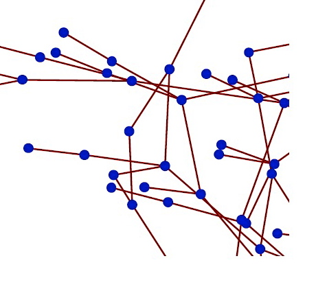
First, the probability regime of the construction of the random graph needs to be specified. Second, more formal definitions of small, middle and large scale are needed. As it is well known, there are different regimes in the model of a random graph:
- (1)
, then the random graph is a large collection of disconnected small trees.
- (2)
with , then all the connected components of the graph are either trees or unicycle components. The giant connected component is a tree and has nodes.
- (3)
with , then a giant component emerges. This one has nodes almost surely where a function depending on and independent on . Also the average degree of a node is bounded away from .
- (4)
with , then the graph is almost surely connected.
Beyond these, for example when , there is a single highly connected component whose average nodal degree is unbounded as .
With these clarifications, we make the following observations. First, random graphs in the (middle) regime are not –hyperbolic, in the sense that they contain –fat triangles for arbitrary large almost surely as . This is proved in Theorem 2.2. This observation was made experimentally in [19] (see the taxonomy chart there) and for which we provide a proof in this work. Figure 2 provides a visualization of this claim. Second, simulations suggest that the proportion of –fat triangles is not only positive but is in fact quite significant for any as grows. These are shown in Section 3.1.

Definition 2.1.
Let be a family of random graphs. We say that a property holds asymptotically almost surely if the probability of this to occur goes to one as .
Theorem 2.2.
For every non–negative , the giant component of with is not –hyperbolic asymptotically almost surely.
Proof.
Let be an Erdös–Renyi random graph with and let be its giant connected component. It is well known that has nodes asymptotically almost surely where is a function on and independent on (see [4] for a proof of this result). Take and let us expose of the nodes of (by exposing we mean to generate the Erdös–Renyi random graph generated by these nodes). We call this set the exposed set. The remaining set of is called the hidden set and is denoted by . It is easy to see that if is such that then the exposed set has a giant connected component of size . Moreover, by taking as before we see that the giant component of the exposed set is contained in the giant component of the whole graph . This is because in the graph there is a unique component of size proportional to all the other components have size .
Let be a node in and let be a positive integer. The probability that has only two neighbors in and no other neighbor is equal to . This probability converges to as . The probability of their neighbors to have another unique neighbor in is asymptotically . Moreover, the probability of the following neighbors to have a unique neighbor and so on until the nodes and (see figure 3) are in the giant component of the exposed set is
| (2.2) |
Where the symbol denotes that the quantities are asymptotically equal.
We say that is the base of a –handle if is a node as in figure 3. Let and be the nodes in the –handle that belong to the giant component of the exposed set. Note that since the nodes and were already in the giant component of the exposed set there exists at least one shortest path connecting them inside the exposed set and not passing through the node . Let be the random variable that is equal to if the node is the base of a –handle with and otherwise.

Let and be the neighbors of and let be the midpoint of the points and (these are the nodes marked in red in the figure) in any path that connects and without passing through . It is clear that the geodesic triangle is at least –fat.
Define to be the random variable . To prove the existence of a –fat triangle in the giant component almost surely it is enough to prove that as . Moreover, we will prove the following stronger result. For every constant , there are almost surely –handles as . Taking in equation (2.2) we obtain that
| (2.3) | |||||
| (2.4) |
Let us define
Then the expected number of –handles in is
| (2.5) | |||||
| (2.6) |
since the random variables are identically distributed and Bernoulli. Since by assumption , we see that this quantity goes to infinity as increases. Let and be two different nodes in and let be the probability of having a –handle based at and another based at . It is rather easy to show that the quotient as . Recall that two random variables and are independent if and only if for all and integers greater or equal than . Since for all then to prove that and are asymptotically independent it is enough to show that . On the other hand,
| (2.7) |
Therefore, we showed that and are asymptotically independent for all .
It is a straightforward calculation to show that the variance satisfies
| (2.8) |
since the random variables and , as we showed, are asymptotically independent. Note that the probability of not having a –handle based at is equal to the probability of . Hence, by Chebyshev’s inequality
By our election of we know that and that as . Therefore, and our result follows. ∎
As a corollary of the previous proof we have an alternative proof of the following known result (e.g., see [11]).
Corollary 2.3.
The giant component of with has no spectral gap asymptotically almost surely.
This result follows because the previously constructed –handles are cut sets with nodes and only two boundary nodes.
3. Simulations
3.1. Numerical Results on Percentage of Fat Triangles
We have seen that random graphs in the regime are almost surely asymptotically non–hyperbolic. However, these random graphs appear to be non–hyperbolic in a much stronger sense. To see how, consider the chart in figure 4. This is an example of a curvature plot (see [19]). For any triangle the corresponding is defined by
| (3.1) |
where is the distance between and the node on that it is closest to. It can be shown (see [2]) that the maximum of over all possible triangles in a graph is finite if and only if the graph is –hyperbolic. Instead of the maximum, figure 4 shows the average value of for all triangles whose shortest side is as a function of Results for random graphs of various sizes, with are shown. The results show a linear increase in saturating at a plateau whose height increases as the size of the graph is increased. The same results are rescaled in the right panel, where all the curves are shifted down and to the left by amounts proportional to Thus the plot shows versus where and are adjusted to achieve the best possible fit. As shown in the figure, except the leftmost part of each curve where , all the curves for different collapse onto a single universal curve. This, together with the fact that the curves in the left panel also coincide before their plateaus implies that the rising part of the universal curve is linear. If , any finite is on the rising part of the universal curve, and therefore increases linearly with with the plateau pushed out to


Thus we see that a significant fraction of triangles in a typical instantiation of are –fat, a stronger demonstration of non–hyperbolicity. Therefore, it seems that –fat triangles not only exist almost surely but they are abundant! Even though we do not yet have direct proof of this observation, figure 4 clearly shows the predominance of fat triangles in due to the increasing (average) . Thus random graphs are far from hyperbolic, contrary to folklore.

Figure 5 shows that if the average for all triangles with the same longest side is plotted as a function of as increases, the height of the curves decreases for small and increases for large with the boundary between the two regions shifting to the right as increases. Thus for any fixed in accordance with the local tree-like structure. Similar results are seen for in figure 6.


3.2. Some Simulation Results on the Bulk Region of the Spectrum
Here we present some simulations of the spectral measure for the Laplacian of the Erdös–Renyi graphs . It is known that these measures converge weakly to a probability measure (see [1]). Observe in figures 7 and 8 how close these probabilities are in the bulk region to the McKay probability measure, the spectral measure of the Laplacian of the –regular tree, that is given by [15] to be
| (3.2) |


It is interesting to compare these plots with the spectral measure of the finite truncated tree. To be more precise, fix and let be the infinite regular tree of degree . The spectral measure for the Laplacian of this tree is given by equation (3.2). Consider now, for each finite the spectral measure of the truncated finite tree constructed from by just keeping only the first generations. It is a well known result (see [10]) that these measures do converge to a measure . However, and are very different. For instance, the measure has atoms while does not. This is due to the fact that repeated eigenvalues occur with large multiplicities. The main heuristic reason for this phenomena is that the truncated tree has a large number of nodes with degree one creating a significant boundary effect. See figure 8 to see this phenomena.
These figures clearly show that the distribution of the spectrum of large Erdös–Renyi random graphs provide a better approximation for the spectral measure of the corresponding infinite regular tree in the bulk region than do large finite truncated trees of the same degree. We do not yet have a complete explanation for this. We note that this result is in contrast to the regime where the distribution of the eigenvalues follow the well-known semi-circle law [5].
Of course the two spectral measures and are not exactly the same; we have shown already that does not have a spectral gap, whereas does. We also observe in figure 7 that the measure for small values of seems to have a spike at 1. As seen in figure 8, the size of this spike seems to decrease as increases, but we do not know if the spike disappears as for fixed small . Nevertheless, the close similarity observed between and naturally raises the question: what is the probability distribution of the measure ? More generally, if we consider the branching process generated by any probability distribution in the natural numbers , what is the spectral measure of the normalized Laplacian for this graph?
Acknowledgement. This work was supported by AFOSR Grant No. FA9550-08-1-0064.
References
- [1] C. Bordenave, M. Lelarge, Resolvent of Large Random Graphs, to appear in Random Structures and Algorithms, http://arxiv.org/0801.0155.
- [2] M. Brisdon, A. Haefliger, Metric Spaces of Non-positive Curvature, Springer Verlag, vol. 319, 1991.
- [3] I. Chavel, Eigenvalues in Riemannian Geometry, Academic Press, Inc., 1984.
- [4] F. Chung, Spectral Graph Theory, CBMS Number 92, AMS, 1994.
- [5] F. Chung, L. Liu, V. Vu, Spectra of Random Graphs with Given Expected Degrees, PNAS vol. 100, no. 11, pp. 6313-6318, 2007.
- [6] A. Coja-Oghlan, A. Lanka, The Spectral Gap of Random Graphs with Given Expected Degrees, The Elect. Journal of Combinatorics, vol. 16, 2009.
- [7] P. Erdös and A. Renyi, Random Graphs I, Publ. Math. Inst. Hungar. Acad. Sci. 6, pp. 290-297, 1959.
- [8] E. Gilbert, Random Graphs, Annals of Mathematical Statistics, vol. 30, no. 4, pp. 1141-1144, 1959.
- [9] M. Gromov, Hyperbolic Groups, Essays in group theory, Springer, New York, pp. 75-263, 1987.
- [10] L. He, X. Liu, G. Strang, Trees with Cantor Eigenvalue Distribution, Studies in Appl. Math. vol. 110, pp. 123-136, 2003.
- [11] B. Itai, G. Kozman, N. Wormald, The Mixing Time of the Giant Component of a Random Graph, http://arxiv.org/0610459v.
- [12] E. Jonckheere, P. Lohsoonthorn, Geometry of Network Security, Proc. of the American Control Conf., 2004.
- [13] B. Karrer, M. Newman, Random Graphs Containing Arbitrary Distribution of Sub-graphs, http://arxiv.org/1005.1659.
- [14] R. Lyons, Y. Peres, Probability on Trees and Networks, Course Notes, Fall 2004 (forthcoming book), http://php.indiana.edu/ rdlyons/prbtree/prbtree.html, 2004.
- [15] B. McKay, The Expected Eigenvalue Distribution of a Large Regular Graph, Lin. Alg. and Applications, vol. 40, pp. 203-216, 1981.
- [16] M. Mezard, A. Montanari, Information, Physics and Computation, Oxford University Press, 2009.
- [17] B. Mohar, The Laplacian Spectrum of Graphs, Graph Theory, Combinatorics, and Appl., vol. 2, pp. 871-898, 1991.
- [18] B. Mohar, W. Woess, A Survey on Spectra of Infinite Graphs, Bull. London Math. Soc., vol. 21, pp. 209-234, 1989.
- [19] O. Narayan, I. Saniee, Large-scale Curvature of Networks, (http://arxiv.org/0907.1478, 2009), Physical Review E (statistical physics), Vol. 84, No. 066108, Dec. 2011.