Integer Point Sets Minimizing Average Pairwise $L_{1}$ Distance: What is the Optimal Shape of a Town?

Selecting an optimal set of locations is a fundamental problem, not just in real estate, but also in many areas of computer science. Typically, the task is to choose $n$ sites from a given set of candidate locations; the objective is to pick a set that minimizes a cost function, e.g., the average distance between sites. As described below, there is a large variety of related results, motivated by different scenarios.

In general, problems of this type are hard, even to approximate, as the problem of finding a clique of given size is a special case. Some of the natural settings have a strong geometric flavor, so it is conceivable that more positive results can be achieved by exploiting additional structures and properties. However, even seemingly easy special cases are still surprisingly difficult. Until now, there was no complexity result (positive or negative) for the scenario in which the candidate locations correspond to the full integer grid, with distances measured by the Manhattan metric (an $n$-town). Indeed, for the shape of area 1 with minimum average $L_{1}$ distance (the “optimal shape of a city”, arising for the limit case of $n$ approaching infinity), no simple closed-form solution is known, suggesting that finding sets of $n$ distinct grid points (the “optimal shapes of towns”) may not be an easy task. This makes the problem mathematically challenging; in addition, the question of choosing $n$ grid positions with minimum average $L_{1}$ distance comes up naturally in grid computing, so the problem is of both practical and theoretical interest.

In this paper, we give the first positive result by describing an $O(n^{7.5})$ algorithm for computing sets of $n$ distinct grid points with minimum average $L_{1}$ distance. Our method is based on dynamic programming, and (despite of its relatively large exponent) for the first time allows computing optimal towns up to $n=80$.

We want to find a set of $n$ distinct points from the integer grid $\mathbb{Z}\times\mathbb{Z}$ such that the sum of all pairwise Manhattan distances is minimized. A set $S\subset\mathbb{Z}\times\mathbb{Z}$ of cardinality $n$ is an $n$-town. An $n$-town $S$ is optimal if its cost

is minimum. Figure 1 shows solutions for small $n$ and their cost, and Table 1 in Section 5 shows optimal cost values $c_{\textrm{town}}(n)$ for $n\leq 80$. We define the $x$-cost $c_{x}(S)$ as $\sum_{\{s,t\}\in S\times S}|s_{x}-t_{x}|$, where $s_{x}$ is the $x$-coordinate of $s$; $y$-cost $c_{y}(S)$ is the sum of all $y$-distances, and $c(S)=c_{x}(S)+c_{y}(S)$. For two sets $S$ and $S^{\prime}$, we define $c(S,S^{\prime})=\sum_{\{s,s^{\prime}\}\in S\times S^{\prime}}\|s-s^{\prime}\|_{1}$. If $S$ consists of a single point $t$, we write $c(t,S^{\prime})$ instead of $c(\{t\},S^{\prime})$ for convenience. A town $S$ is convex if the set of grid points in the convex hull of $S$ equals $S$.

In proving various properties of optimal towns, we will often make a local modification by moving a point $t$ of a town to a different place $r$. The next lemma expresses the resulting cost change.

The following proof holds in any dimension and with any norm for measuring the distance between points.

Obviously, if we translate every point from an $n$-town by the same vector, the cost of the town does not change. We want to distinguish towns because of their shape and not because of their position inside the grid and, therefore, we will only consider optimal towns that are placed around the origin. Lemma 3 makes this more precise: an optimal $n$-town is roughly symmetric with respect to a vertical and a horizontal symmetry line, see Fig. 2 for an illustration. Perfect symmetry is not possible since some rows or columns may have odd length and others even length.

We need some notation before: For an $n$-town $S$, the $i$-th column of $S$ is the set $C_{i}=\{\,(i,y)\in S:y\in\mathbb{Z}\,\}$ and the $i$-th row of $S$ is the set $R_{i}=\{\,(x,i)\in S:x\in\mathbb{Z}\,\}$.

From the convexity statement in Lemma 2 (together with Lemma 3) we know that $C_{0}$ is the largest column, and the column lengths decrease to both sides, and similarly for the rows. Our algorithm will only be based on this weaker property (orthogonal convexity); it will not make use of convexity per se. We will, however, use convexity one more time to prove that the lengths of the columns are $O(\sqrt{n})$, in order to reduce the running time.

In the following we assume the symmetry property of the last lemma. For an $n$-town $S$, let the width of $S$ be $w(S)=\max_{i\in\mathbb{Z}}|R_{i}|$ and the height of $S$ be $h(S)=\max_{i\in\mathbb{Z}}|C_{i}|$. We will now show that the width and the height cannot differ by more than a factor of 2. Together with convexity, this will imply that they are bounded by $O(\sqrt{n})$ (Lemma 5).

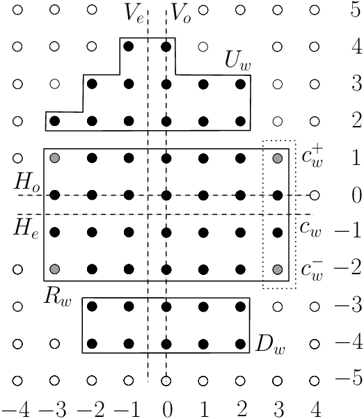
We will now describe a dynamic-programming algorithm for computing optimal towns. A program for this algorithm is listed in A.

We denote by $c_{i}=|C_{i}|$ the number of selected points in column $i$ and by $c_{i}^{+}$ and $c_{i}^{-}$ the row index of the topmost and bottommost selected point in $C_{i}$, respectively. We have $c_{i}=c_{i}^{+}-c_{i}^{-}+1$; see Fig. 2.

Now we describe the dynamic program. It starts with the initial empty grid and chooses new columns alternating from the set of columns with nonnegative and with negative column index, i.e., in the order $0,-1,1,-2,2,\ldots$. Let $w\geq 0$ be the index of the currently chosen column and fix $c_{w}$ to a value $c$. We describe the dynamic program for columns with nonnegative index; columns with negative index are handled similarly. (In the program that is described in the appendix, we use a trick to avoid dealing with negative columns: they are mapped to columns with positive index by reflecting everything at the $y$-axis, with a proper adjustment to take into account that the placement of Lemma 3 is not invariant under this transformation.)

We know from Lemma 6 that in every optimal solution, every point inside the rectangle $R_{w}=[-w,w]\times[c_{w}^{-},c_{w}^{+}]$ is selected. We define

as the minimum cost of a town with columns $-w,\ldots,w$ of height $c_{i}\geq c$ for $-w\leq i\leq w$ and $c_{w}=c$ where $U_{w}$ points lie above the rectangle $R_{w}$, having a total distance $\Delta_{w}^{\mathrm{UL}}$ and $\Delta_{w}^{\mathrm{UR}}$ to the upper-left and upper-right corner of $R_{w}$, respectively, and $D_{w}$ points lie below $R_{w}$, having a total distance $\Delta_{w}^{\mathrm{DL}}$ and $\Delta_{w}^{\mathrm{DR}}$ to the lower-left and lower-right corner of $R_{w}$. For a given $n$, we are looking for the $n$-town with minimum cost where $(2w+1)c+U_{w}+D_{w}=n$. Next we show that $\cost(w,c,\Delta_{w}^{\mathrm{UR}},\Delta_{w}^{\mathrm{DR}},\Delta_{w}^{\mathrm{UL}},\Delta_{w}^{\mathrm{DL}},U_{w},D_{w})$ can be computed recursively.

Consider the current column $w$ with $c_{w}=c$. The cost from all points in this column to all points above $R_{w}$, in $R_{w}$, and below $R_{w}$ can be expressed as

We can transform this into

which, obviously, depends only on the parameters $w$, $c$, $\Delta_{w}^{\mathrm{UR}}$, $\Delta_{w}^{\mathrm{DR}}$, $U_{w}$, and $D_{w}$ (the two parameters $\Delta_{w}^{\mathrm{UL}}$, $\Delta_{w}^{\mathrm{DL}}$ are needed if we consider a column with negative index). We denote the expression (2) by $\dist(w,c,\Delta_{w}^{\mathrm{UR}},\Delta_{w}^{\mathrm{DR}},\allowbreak\Delta_{w}^{\mathrm{UL}},\allowbreak\Delta_{w}^{\mathrm{DL}},\allowbreak U_{w},\allowbreak D_{w})$ and state the recursion for the cost function:

By Lemma 6 it suffices to consider only previous solutions with $c_{-w}\geq c$. In the step before, we considered the rectangle $R_{-w}=[-w,w-1]\times[c_{-w}^{+},c_{-w}^{-}]$. Hence, the parameters with index $-w$ can be computed from the parameters with index $w$ as follows:

The parameters $\Delta_{-w}^{\mathrm{UL}}$ and $\Delta_{-w}^{\mathrm{DL}}$ can be computed analogously and the cost function is initialized as follows:

The bound on $c$ has been shown in Lemma 5.

For large values of $n$, $n$-towns converge towards the continuous weight distributions of cities. However, the arrangement of buildings in many cities are discretized in a different sense: An $n$-block city is the union of $n$ axis-aligned unit squares (“city blocks”), see Fig. 3 below. In the following, we discuss $n$-block cities, and we discuss the relation between $n$-towns and $n$-block cities.

For a planar region $R$, let $c^{\prime}(R)$ be the integral of Manhattan distances between all point pairs in $R$:

When $R$ has area 1, this is the expected distance between two random points in $R$. Scaling a shape $R$ by a factor of $d$ increases the total cost by a factor of $d^{5}$, i.e., by a factor of $A^{2.5}$ for an area of $A$. This motivated Bender et al. (2004) to use the expression $D(R):=\frac{c^{\prime}(R)}{A(R)^{2.5}}$ as a scale-independent measure for the quality of the shape of a city. For example, a square $Q$ of any side length $a$ gets the same value

A circle $C$ yields $D(C)=\frac{512}{45\pi^{2.5}}\approx 0.6504$ and the optimal shape achieves a value of $\psi=0.650\,245\,952\,951\ldots$

We will consider $n$-block cities $Q(S)$ consisting of unit squares (“blocks”) centered at a set of $n$ grid points $S\subset\mathbb{Z}\times\mathbb{Z}$. We denote a unit square centered at point $s=(s_{x},s_{y})$ by $Q(s)=[s_{x}-\frac{1}{2},s_{x}+\frac{1}{2}]\times[s_{y}-\frac{1}{2},s_{y}+\frac{1}{2}]$, and then we have

The average distance $D(Q(S))$ of an $n$-block city can be decomposed into average distances between blocks:

Using the notation

we can express this as

The average distance $d^{\prime}(s)$ between two square blocks at an offset $s$ can be expressed as follows: If the two blocks don’t lie in the same row or column ($s_{x}\neq 0$ and $s_{y}\neq 0$), the average distance is simply the distance $\lVert s\rVert_{1}$ between the centers, since positive and negative deviations from the block centers average out. When two blocks lie in the same column, then the $y$-distances average out to the $y$-distance between the centers, but the average $x$-distance is not the $x$-distance between the centers (which would be 0), but $\int_{-1/2}^{+1/2}\int_{-1/2}^{+1/2}|x_{1}-x_{2}|\,dx_{2}\,dx_{1}=\frac{1}{3}$. Similarly, for two blocks in the same row, we must add $\frac{1}{3}$ to the distance $\lVert s\rVert_{1}$ between the centers. Finally, for two identical blocks, we have already seen that the average distance is $\frac{2}{3}$. We can express this compactly as

where the notation $[s_{x}\neq 0]$ is 1 if the predicate $s_{x}\neq 0$ holds and 0 otherwise. With these conventions, the expression (4) for the cost $c^{\prime}(Q(S))$ of an $n$-block city $Q(S)$ looks very similar to (1) for the cost $c(S)$ of a town $S$, except for the correction terms $\frac{1}{3}$ in the summands and for the factor $\frac{1}{2}$. The factor $\frac{1}{2}$ accounts for the fact that in the sum $c(S)$ of a town, each pair of (distinct) points is counted once, whereas in the integral $c^{\prime}(R)$, each pair of points is considered twice, as two ordered pairs. To make these expressions better comparable, we introduce the factor $\frac{1}{2}$ and define

The new “distance” $d^{\prime}$ is not a norm (for example, $d^{\prime}(0)\neq 0$), but the properties from Section 2 remain true for this new objective function. Thus, the dynamic programming formulation of Section 3 can be adapted to compute optimal $n$-block cities. As we shall now demonstrate, all lemmas of Section 2 hold verbatim for $n$-block cities, except that the formula for the change incurred by moving a single block to a different place (Lemma 1) must be adapted:

The proof is the same as for Lemma 1. One can easily check that the distance $d^{\prime}$ from $t$ to itself and the distance from $r$ to itself are correctly accounted for. ∎

Convexity of the optimum solution (Lemma 2) holds true for $n$-block cities. The proof goes through almost verbatim. The expression $d^{\prime}(p)$ is not a norm, but it is a convex function of $p$, and this is all that is needed. Approximate symmetry of the optimal solution (Lemma 3) remains true. The calculations (which have not been shown in detail anyway), are modified, but the conclusion is the same.

When comparing an $n$-town $S$ and a corresponding $n$-block city $Q(S)$, we have to add 1/6 for each pair of blocks that are in the same column, and for each pair of blocks that are in the same row. Using the notation $r_{j}$ and $c_{i}$ of Section 3 for row and column lengths, and writing $c_{\textrm{town}}(S)$ instead of $c(S)$ for improved clarity, we get thus:

This adjustment term accounts for the discretization effect. For example, a $1$-town has an average distance of 0, as all the weight is concentrated in a single point, while a $1$-block city has an average distance of $2/3$, just like any other square, (and a $c_{\textrm{city}}$ value of $1/3$).

Using this expression, it is easy to show that the bound of 2 on the aspect ratio holds for $n$-block cities in the same form as in Lemma 4. The proof of Lemma 4 establishes that $c_{\textrm{town}}(S)$ decreases when a top-most point $t$ from the longest column of height $h$ is added to the right of the longest row of length $w$. For an $n$-block city, the adjustment term $\Lambda(S)$ decreases by at least $h^{2}-(h-1)^{2}$ when $t$ is removed, and it increases by $(w+1)^{2}-w^{2}+1^{2}$ when $r$ is added. Under the assumption of the proof ($w\leq h/2-3$), the total change of $\Lambda$ is negative, and the modified solution is an improvement also when $S$ is regarded as an $n$-block city.

From Lemma 4 we conclude that the bound of $2\sqrt{n}+5$ on the height and width of optimal $n$-block cities (Lemma 5) holds as well. (The argument of the proof of Lemma 5 is purely geometric: it is based on convexity and does not use the objective function.)

Thus, we conclude that the adjustment term (5) is asymptotically bounded by $\Lambda(S)=\Theta(n^{1.5})$.

When considering the continuous weight distributions of $n$-block cities, we have to account twice for each pair of discrete block centers; hence, the appropriate measure for the quality of an $n$-town is $\Phi(S)={2c(S)}/{n^{2.5}}$. The measure for the corresponding $n$-block city is $\Psi(S)={2(c_{\mathrm{town}}(S)+\Lambda(S))}/{n^{2.5}}$. Thus, the relative difference is $\Theta(\frac{1}{n})$.

In Figure 3, we show the corresponding values for the small examples from Figure 1. Figure 5 shows results for some larger values $n$. One can observe how $\Phi(S)$ and $\Psi(S)$ converge from below and above towards the optimal city value $\psi$ of about 0.650 245 952 951. Note that convergence is not monotone, neither for $\Phi$ nor for $\Psi$.

Optimal $n$-towns and optimal $n$-block cities do not necessarily have the same shape. For $n\leq 21$, a comparison of Figures 1 and 3 shows that, while not all optimal $n$-towns are optimal $n$-block cities, every optimal $n$-block city is simultaneously an optimal $n$-town. However, this is not always true. In fact, for $n=72$, there are two shapes for optimal $n$-block cities, none of which is optimal for an $n$-town, see Figure 4. This is the only instance of this phenomenon up to $n=80$, but we surmise it will be more and more frequent for larger $n$. We have more comments on this phenomenon at the end of this section.

References

- Arora et al. (1999) Arora, S., Karger, D. R., Karpinski, M., 1999. Polynomial time approximation schemes for dense instances of NP-hard problems. J. Comput. Syst. Sci. 58 (1), 193–210.
- Asahiro et al. (2000) Asahiro, Y., Iwama, K., Tamaki, H., Tokuyama, T., 2000. Greedily finding a dense subgraph. J. Algorithms 34 (2), 203–221.
- Bartal et al. (2001) Bartal, Y., Charikar, M., Raz, D., 2001. Approximating min-sum -clustering in metric spaces. In: Proc. 33rd Symp. on Theory of Computation. pp. 11–20.
- Bender et al. (2004) Bender, C. M., Bender, M. A., Demaine, E. D., Fekete, S. P., 2004. What is the optimal shape of a city? Journal of Physics A: Mathematical and General 37, 147–159.
- Bender et al. (2008) Bender, M. A., Bunde, D. P., Demaine, E. D., Fekete, S. P., Leung, V. J., Meijer, H., Phillips, C. A., 2008. Communication-aware processor allocation for supercomputers: Finding point sets of small average distance. Algorithmica 50 (2), 279–298.
- Fekete and Meijer (2003) Fekete, S. P., Meijer, H., 2003. Maximum dispersion and geometric maximum weight cliques. Algorithmica 38, 501–511.
- Fekete et al. (2005) Fekete, S. P., Mitchell, J. S. B., Beurer, K., 2005. On the continuous Fermat-Weber problems. Operations Research 53, 61–76.
- Fekete et al. (2000) Fekete, S. P., Mitchell, J. S. B., Weinbrecht, K., 2000. On the continuous Weber and -median problems. In: Proceedings of the 16th Annual Symposium on Computational Geometry (SoCG). pp. 70–79.
- Guttmann-Beck and Hassin (1998) Guttmann-Beck, N., Hassin, R., 1998. Approximation algorithms for minimum sum -clustering. Disc. Appl. Math. 89, 125–142.
- Hassin et al. (2009)
Hassin, R., Levin, A., Sviridenko, M., 2009. Approximating minimum quadratic
assignment problems. To appear.
URL http://www.research.ibm.com/people/s/sviri/papers/qa5.p%df - Hassin et al. (1997) Hassin, R., Rubinstein, S., Tamir, A., 1997. Approximation algorithms for maximum dispersion. Oper. Res. Lett. 21 (3), 133–137.
- Indyk (1999) Indyk, P., 1999. A sublinear time approximation scheme for clustering in metric spaces. In: Proc. 40th Annual IEEE Symp. Found. Comp. Science (FOCS). pp. 154–159.
- Karp et al. (1975) Karp, R. M., McKellar, A. C., Wong, C. K., 1975. Near-optimal solutions to a 2-dimensional placement problem. SIAM J. Comput. 4 (3), 271–286.
- Kortsarz and Peleg (1993) Kortsarz, G., Peleg, D., 1993. On choosing a dense subgraph. In: IEEE (Ed.), Proceedings of the 34th Annual Symposium on Foundations of Comptuer Science. IEEE Computer Society Press, Palo Alto, CA, pp. 692–703.
- Krumke et al. (1997) Krumke, S., Marathe, M., Noltemeier, H., Radhakrishnan, V., Ravi, S., Rosenkrantz, D., 1997. Compact location problems. Theoret. Comp. Sci. 181 (2), 379–404.
- Leung et al. (2002) Leung, V., Arkin, E., Bender, M., Bunde, D., Johnston, J., Lal, A., Mitchell, J., Phillips, C., Seiden, S., 2002. Processor allocation on Cplant: Achieving general processor locality using one-dimensional allocation strategies. In: Proc. 4th IEEE International Conference on Cluster Computing. pp. 296–304.
- Loiola et al. (2007) Loiola, E. M., de Abreu, N. M. M., Netto, P. O. B., Hahn, P., Querido, T. M., 2007. A survey for the quadratic assignment problem. European Journal of Operational Research 176 (2), 657–690.
- Mache and Lo (1996) Mache, J., Lo, V., 1996. Dispersal metrics for non-contiguous processor allocation. Technical Report CIS-TR-96-13, University of Oregon.
- Mache and Lo (1997) Mache, J., Lo, V., 1997. The effects of dispersal on message-passing contention in processor allocation strategies. In: Proc. Third Joint Conference on Information Sciences, Sessions on Parallel and Distributed Processing. Vol. 3. pp. 223–226.
- Ravi et al. (1994) Ravi, S. S., Rosenkrantz, D. J., Tayi, G. K., 1994. Heuristic and special case algorithms for dispersion problems. Operations Research 42 (2), 299–310.
- Sahni and Gonzalez (1976) Sahni, S., Gonzalez, T., 1976. -complete approximation problems. Journal of the ACM 23 (3), 555–565.
n_target = 40 # run up to this value of n
cost_array = {} # initialize data for "array"
from math import sqrt
width_limit = int(2*sqrt(n_target)+5)
for w in range(0,width_limit+2):
for cc in range(width_limit,0,-1):
cost_array[w,cc]={}
MAX = n_target**3 # "infinity", trivial upper bound on cost
opt = (n_target+1)*[MAX] # initialize array for optimal values
cost_array[0,width_limit][0,0,0,0,0,0]=0 # starting "town" with no columns
for w in range(0,width_limit+1):
for (D_up_right, D_down_right, D_up_left, D_down_left,
n_up, n_down), cost in cost_array[w,cc].items():
D_up_left   += n_up # add 1 horizontal unit to all left-distances
D_down_left += n_down
for c in range(cc,-1,-1): # decrease size c of new column one by one
n = n_up+n_down + (w+1)*c # (w = previous value of w)
if n <= n_target: # total number of occupied points so far
new_cost = cost + ( (D_up_left + D_down_left) * c +
(n_up + n_down) * c*(c-1)/2 +
(c+1)*c*(c-1)/6 * (2*w+1) +
c*c * w*(w+1)/2 )
if c==0: # a completed town
opt[n] = min( new_cost, opt[n] )
else: # store cost of newly constructed partial town
ind = (D_up_left, D_down_left, D_up_right, D_down_right,
n_up, n_down) # exchange left and right when storing
cost_array[w+1, c][ind] = min ( new_cost,
cost_array[w+1, c].get(ind, MAX) )
# decrease c by 1:
if (c%2)==1: # remove an element from the top of the leftmost column
n_up += w
D_up_left  += n_up + w*(w+1)/2
D_up_right += n_up + w*(w-1)/2
else: # remove from the bottom
n_down += w
D_down_left  += n_down + w*(w+1)/2
D_down_right += n_down + w*(w-1)/2
for n in range(1,n_target+1): print n, opt[n]
Appendix A Program for Computing Optimal Towns
Figure 6 shows a short program in the programming language Python that
implements our algorithm.
The program calculates and prints the costs of optimal -towns for
all values of
up to the specified limit .
Instead of an 8-dimensional array, the
costs are stored as a dictionary in the variable
cost_array[w,cc][D_up_right, D_down_right, D_up_left, D_down_left,
n_up, n_down].
This makes the program a lot simpler, since we don’t have to worry about
allocating arrays with explicit limits, and
incurs little overhead, since internally, Python dictionaries
are implemented as hash tables, providing constant expected access time.
Instead of adding rows alternately on the left and on the right, the program always adds a new row on the left side, but (implicitly) reflects the town about the -axis when storing a cost value, achieving the same effect.
The main loop of the program does not use the recursion in the
form (3), which calculates the optimum cost of a
configuration from all partial solution that lead to it when a column
is added. Instead, it makes a “forward” transfer, generating
all successor configurations of a given configuration. This has the
advantage that certain “impossible” parameter sets are automatically
excluded. For example, in the running time analysis for
Theorem 7, we argued that parameter pairs with
need not be considered.
(The parameters and correspond to the variables n_up and n_down.)
Since the program only
adds columns which are (approximately) balanced about the -axis,
it will never generate solutions with such parameters.
The program can be adapted for computing optimal -block
cities. Then the additional cost
from (5)
between blocks in the same row or column must be
taken into account. One simply has to extend the last line in the
computation of new_cost:
to
c*c * w*(w+1)/2 ) * 6 + c*c + (cc-c)*w*w
The resulting cost is scaled by a factor of 6, but the end result is then always even, so we could divide it by 2 (cf. Table 1: all values are multiples of ).
For , the program takes a few seconds, but for it takes
hours.
For larger the space becomes a more severe bottleneck than
the running time; thus it is important to release
storage when it is no longer needed, for
example by resetting cost_array[w,cc]={}
after each outer loop.
There are several possibilities to speed up the program.
The cost of some approximately circular solution can be taken as an
initial upper bound. With this upper bound, one can then derive a
stronger bound width_limit on the maximum height and width by
ad-hoc methods. During the calculation, one can also prune cost
values that are so large that they cannot possibly lead to a better
solution. The given program computes only the optimum cost. We have
extended it to also remember the optimal solutions. This program has
133 lines and was used to produce the data of