跳到论文正文
W Papers独立论文阅读器 arXiv:1009.5587 论文正文 计算阅读时间 · 0%
引用这篇论文根据当前论文元数据生成,正式投稿前建议核对。


License: arXiv.org perpetual non-exclusive license
arXiv:1009.5587v3 [cond-mat.str-el] 15 Nov 2011

Boundary effects on the local density of states of one-dimensional
Mott insulators and charge density wave states

Dirk Schuricht Affiliation: Institute for Theory of Statistical Physics, RWTH Aachen, 52056 Aachen, Germany Affiliation: JARA-Fundamentals of Future Information Technology    Fabian H. L. Essler Affiliation: The Rudolf Peierls Centre for Theoretical Physics, University of Oxford, 1 Keble Road, OX1 3NP, Oxford, UK    Akbar Jaefari Affiliation: Department of Physics, University of Illinois at Urbana-Champaign, 1110 W. Green St, Urbana, Illinois 61801-3080, USA    Eduardo Fradkin Affiliation: Department of Physics, University of Illinois at Urbana-Champaign, 1110 W. Green St, Urbana, Illinois 61801-3080, USA
August 24, 2026
Abstract

We determine the local density of states (LDOS) for spin-gapped one-dimensional charge density wave (CDW) states and Mott insulators in the presence of a hard-wall boundary. We calculate the boundary contribution to the single-particle Green function in the low-energy limit using field theory techniques and analyze it in terms of its Fourier transform in both time and space. The boundary LDOS in the CDW case exhibits a singularity at momentum 2​kF2k_{\mathrm{F}}, which is indicative of the pinning of the CDW order at the impurity. We further observe several dispersing features at frequencies above the spin gap, which provide a characteristic signature of spin-charge separation. This demonstrates that the boundary LDOS can be used to infer properties of the underlying bulk system. In presence of a boundary magnetic field mid-gap states localized at the boundary emerge. We investigate the signature of such bound states in the LDOS. We discuss implications of our results on STM experiments on quasi-1D systems such as two-leg ladder materials like Sr14Cu24O41. By exchanging the roles of charge and spin sectors, all our results directly carry over to the case of one-dimensional Mott insulators.

I Introduction

Scanning tunneling microscopy (STM) and spectroscopy (STS) methods have proved to be a useful tool for studying strongly correlated electron systems such as carbon nanotubes [1], high temperature superconductors (HTSC) [2, 3, 4, 5] and rare-earth compounds [6]. STM experiments measure the tunneling current II between the sample and the STM tip as a function of its position xx and the applied voltage VV. This current can be expressed in terms of the local densities of states (LDOS) in the sample N⁡(E,x)N(E,x) and the tip Ntip​(E)N_{\mathrm{tip}}(E) as [5]

I⁡(V,x)∝∫d​E​[f⁡(E−e​V)−f⁡(E)]​Ntip​(E−e​V)​N​(E,x),I(V,x)\propto\int dE\,\bigl[f(E-eV)-f(E)\bigr]\,N_{\mathrm{tip}}(E-eV)\,N(E,x), (1)

where f⁡(E)f(E) denotes the Fermi function. Assuming a structureless density of states in the tip, Ntip=constN_{\mathrm{tip}}=\text{const}, this gives the following expression for the local tunneling conductance

d​I​(V,x)d​V∝∫d​E​f′​(E−e​V)​N​(E,x).\frac{dI(V,x)}{dV}\propto\int dE\,f^{\prime}(E-eV)\,N(E,x). (2)

Eq. (2) shows that the tunneling conductance is proportional to the thermally smeared N⁡(E,x)N(E,x) of the sample at the position of the tip. A non-trivial spatial dependence of the LDOS arises in presence of impurities. These break translational invariance and lead to a modification of the LDOS in their vicinity, from which one can infer characteristic properties of the bulk state of matter as well as the nature of its electronic excitations. Spatial modulations of the LDOS can be analyzed in terms the Fourier transform of the tunneling conductance. It follows from (2) that this quantity is directly proportional to the corresponding Fourier transform of the LDOS, N⁡(E,Q)N(E,Q). This method of analyzing STM data was used very successfully [3] to study quasiparticle interference in Bi2Sr2CaCu2O8+δ. The spin dependence of the LDOS has also been investigated using magnetic tips[7]. Theoretical studies of STS have focused in particular on Luttinger liquids[8, 9] and HTSC[9, 10, 11]. In the Luttinger liquid case an impurity has the same effects at low energies as a physical boundary[12], which motivated studies of the LDOS in the vicinity of a chain end. The case of strongly correlated one-dimensional (1D) systems with spin or charge gaps is of considerable interest as well and pertains to quasi 1D charge density wave (CDW) systems[13] and Mott insulators[15, 14], carbon nanotubes[16], (doped) two-leg ladder materials[17, 18], and the stripe phases of HTSC[19]. As compared to the Luttinger liquid case the presence of an interaction-induced gap makes these problems much more difficult to treat theoretically. In the following we will determine the LDOS for the low-energy limit of 1D CDW states and Mott insulators in presence of a single boundary. The latter can be thought of as arising as the result of the presence of a strong potential impurity. Alternatively one can imagine inducing a boundary in a two tip STM setup, where the first tip is used to induce a boundary by applying a high voltage and the LDOS is then measured with a second tip. A short summary of our results has appeared previously[20].

The outline of this paper is as follows: in section II we present the field theory limit of 1D CDW states and Mott insulators in presence of a single boundary. In section III we summarize our results for the single-particle Green function. These are then used to determine the Fourier transform Nσ​(E,Q)N_{\sigma}(E,Q) of the local density of states for hard-wall boundary conditions in section IV. Signatures of spin and charge excitations visible in Nσ​(E,Q)N_{\sigma}(E,Q) are discussed in some detail. The effects of more general boundary conditions, including the formation of boundary bound states, are described in section V. Section VI deals with the effects of finite temperatures and implications of our results for STM experiments are discussed in section VII. The technical details of our calculations are presented in several appendices.

II The model

Our analysis of the LDOS is based on the continuum description of certain 1D CDW states and Mott insulators. The resulting quantum field theory for both cases is known as the U(1) Thirring model[21] (with two “flavors”.) The latter is known to arise as the effective low-energy description of a number of lattice models of spin-1/21/2 electrons as we discuss next.

  1. 1.

    Half-filled repulsive Hubbard model [22]:

    This is the standard model for single band 1D Mott insulators. The Hamiltonian is of the form

    H\displaystyle H =\displaystyle= −t∑j,σ[cj,σ†cj+1,σ+cj+1,σ†cj,σ]+U∑j(nj,↑−12)(nj,↓−12),\displaystyle-t\sum_{j,\sigma}\left[c^{\dagger}_{j,\sigma}c_{j+1,\sigma}+c^{\dagger}_{j+1,\sigma}c_{j,\sigma}\right]+U\sum_{j}\left(n_{j,\uparrow}-\frac{1}{2}\right)\left(n_{j,\downarrow}-\frac{1}{2}\right), (3)

    where nj,σ=cj,σ†​cj,σn_{j,\sigma}=c^{\dagger}_{j,\sigma}c_{j,\sigma} and nj=nj,↑+nj,↓n_{j}=n_{j,\uparrow}+n_{j,\downarrow} are electron number operators and U>0U>0.

  2. 2.

    1D Holstein model [23]:

    The Holstein model provides an example of an incommensurate CDW state and describes a partially filled band of spin-1/21/2 electrons coupled to dispersionless phonons of frequency ω0=kM\omega_{0}=\sqrt{\frac{k}{M}}

    H=−t∑j,σ[cj,σ†cj+1,σ+cj+1,σ†cj,σ]+∑j[Pj22​M+k2Qj2]−λ∑j,σQjnj,σ.\displaystyle H=-t\sum_{j,\sigma}\left[c^{\dagger}_{j,\sigma}c_{j+1,\sigma}+c^{\dagger}_{j+1,\sigma}c_{j,\sigma}\right]+\sum_{j}\left[\frac{P_{j}^{2}}{2M}+\frac{k}{2}Q_{j}^{2}\right]-\lambda\sum_{j,\sigma}Q_{j}n_{j,\sigma}. (4)

    Integrating out the phonons induces a retarded attractive electron-electron interaction. In the limit t≪ω0t\ll\omega_{0} the retardation effects can be neglected, leading to an effective attractive Hubbard model with U∝−λ2U\propto-\lambda^{2}.

  3. 3.

    Su-Schrieffer-Heeger model [24]:

    A second example of an incommensurate CDW state is provided by the Su-Schrieffer-Heeger model, which describes a partially filled band of spin-1/21/2 electrons coupled to dispersing phonons

    H=−∑j,σ[t−λ(Qj+1−Qj)][cj,σ†cj+1,σ+cj+1,σ†cj,σ]+∑j[Pj22​M+k2[Qj+1−Qj]2].\displaystyle H=-\sum_{j,\sigma}\bigl[t-\lambda(Q_{j+1}-Q_{j})\bigr]\left[c^{\dagger}_{j,\sigma}c_{j+1,\sigma}+c^{\dagger}_{j+1,\sigma}c_{j,\sigma}\right]+\sum_{j}\left[\frac{P_{j}^{2}}{2M}+\frac{k}{2}\left[Q_{j+1}-Q_{j}\right]^{2}\right]. (5)

    Taking the continuum limit of (5) (which describes the behavior at low frequencies ω≲t\omega\lesssim t) it was shown by Fradkin and Hirsch [25] that the regime of large phonon frequencies t≪ω0=kMt\ll\omega_{0}=\sqrt{\frac{k}{M}} is described by the U(1) Thirring model[21, 26].

In all three cases a continuum description of the low-energy electronic degrees of freedom is obtained by considering only the modes in the vicinity of the Fermi points ±kF\pm k_{\mathrm{F}}. The lattice electron annihilation operators are expressed in terms of slowly varying right- and left-moving Fermi fields as

cj,σa0→Ψσ​(x)=ei​kF​x​Rσ​(x)+e−i​kF​x​Lσ​(x),\frac{c_{j,\sigma}}{\sqrt{a_{0}}}\rightarrow\Psi_{\sigma}(x)=e^{\text{i}k_{\mathrm{F}}x}R_{\sigma}(x)+e^{-\text{i}k_{\mathrm{F}}x}L_{\sigma}(x), (6)

where a0a_{0} is the lattice spacing, x=j​a0x=ja_{0}, and σ=↑,↓\sigma=\uparrow,\downarrow labels the spin. In the bulk the fields RσR_{\sigma} and LσL_{\sigma} are bosonized according to

Rσ†​(τ,x)\displaystyle R^{\dagger}_{\sigma}(\tau,x) =\displaystyle= ησ2​π​exp⁡(i2​ϕc​(τ,x))​exp⁡(i2​fσ​ϕs​(τ,x)),\displaystyle\frac{\eta_{\sigma}}{\sqrt{2\pi}}\,\exp\Bigl(\tfrac{\text{i}}{2}\phi_{\mathrm{c}}(\tau,x)\Bigr)\,\exp\Bigl(\tfrac{\text{i}}{2}f_{\sigma}\phi_{\mathrm{s}}(\tau,x)\Bigr), (7)
Lσ†​(τ,x)\displaystyle L^{\dagger}_{\sigma}(\tau,x) =\displaystyle= ησ2​π​exp⁡(−i2​ϕ¯c​(τ,x))​exp⁡(−i2​fσ​ϕ¯s​(τ,x)),\displaystyle\frac{\eta_{\sigma}}{\sqrt{2\pi}}\,\exp\Bigl(-\tfrac{\text{i}}{2}\bar{\phi}_{\mathrm{c}}(\tau,x)\Bigr)\,\exp\Bigl(-\tfrac{\text{i}}{2}f_{\sigma}\bar{\phi}_{\mathrm{s}}(\tau,x)\Bigr), (8)

where the Klein factors ησ\eta_{\sigma} satisfy anticommutation rules {ησ,ησ′}=2​δσ​σ′\left\{\eta_{\sigma},\eta_{\sigma}^{\prime}\right\}=2\delta_{\sigma\sigma^{\prime}} and f↑=1=−f↓f_{\uparrow}=1=-f_{\downarrow}. The fields ϕa\phi_{a} and ϕ¯a\bar{\phi}_{a} are the chiral components of the canonical Bose fields Φa\Phi_{a} and their dual fields Θa\Theta_{a},

Φa=ϕa+ϕ¯a,Θa=ϕa−ϕ¯a,a=c,s.\Phi_{a}=\phi_{a}+\bar{\phi}_{a},\;\Theta_{a}=\phi_{a}-\bar{\phi}_{a},\quad a=\mathrm{c},\mathrm{s}. (9)

In the bulk the Hamiltonian density then can be cast in the spin-charge separated form

ℋ⁡(x)\displaystyle{\cal H}(x) =\displaystyle= ∑a=c,sℋa​(x),\displaystyle\sum_{a=\mathrm{c,s}}{\cal H}_{a}(x),
ℋa\displaystyle{\cal H}_{\rm a} =\displaystyle= va16​π[1Ka2(∂xΦa)2+Ka2(∂xΘa)2]−ga(2​π)2cosΦa,\displaystyle\frac{v_{a}}{16\pi}\biggl[\frac{1}{K_{a}^{2}}\bigr(\partial_{x}\Phi_{a}\bigr)^{2}+K_{a}^{2}\bigr(\partial_{x}\Theta_{a}\bigr)^{2}\biggr]-\frac{g_{a}}{(2\pi)^{2}}\ \cos\Phi_{a}, (10)

The charge and spin velocities vc,sv_{\mathrm{c,s}}, the Luttinger parameters Kc,sK_{\mathrm{c,s}} and coupling constants gc,sg_{\mathrm{c,s}} are functions of the hopping integrals and interaction strengths defining the underlying microscopic model. The cases discussed above correspond to the following parameter regimes:

  1. 1.

    Mott insulators

    As a result of repulsive electron-electron interactions we have vc>vsv_{\mathrm{c}}>v_{\mathrm{s}} and Kc<1K_{\mathrm{c}}<1. The cos⁡Φc\cos\Phi_{\mathrm{c}} perturbation in the charge sector is relevant and opens up a gap. The cos⁡Φs\cos\Phi_{\mathrm{s}} interaction in the spin sector is marginally irrelevant and flows to zero under the renormalization group. We therefore neglect it in the following.

  2. 2.

    Electron-Phonon Systems

    At low energies the electron-phonon coupling induces an attractive electron-electron interaction, which results in vs>vcv_{\mathrm{s}}>v_{\mathrm{c}} and Kc>1>KsK_{\mathrm{c}}>1>K_{\rm s}. The cos⁡Φc\cos\Phi_{\mathrm{c}} term is irrelevant, while cos⁡Φs\cos\Phi_{\mathrm{s}} term is relevant (marginally relevant in the spin-SU(2) symmetric case Ks=1K_{\mathrm{s}}=1) and opens up a gap in the spin sector.

In both cases we end up with a spin-charge separated theory of a gapless Luttinger liquid and a sine-Gordon model.

We now imagine a strong, local potential to be present. It is well known from the work of Kane and Fisher[12] that the coupling to the impurity is relevant, leading to a crossover at a characteristic dynamical energy (and temperature) scale called “TKT_{\mathrm{K}}”, below which the system is effectively cut into two disconnected parts, and to a pinning of the CDW. This potential could be due to a strong potential impurity or an STM tip. We model the strong impurity potential by a boundary condition on the continuum electron field

Ψσ​(x=0)=0.\Psi_{\sigma}(x=0)=0. (11)

An important physical consequence of the pinning of the CDW at the impurity (or boundary) is the development of an induced static CDW order in this (effectively) quantum critical system. This induced static CDW order, often referred to[27] as a “Friedel oscillation”, leads to non-dispersive features in the LDOS[9] which can be detected in STM and STS experiments.

Our effective low-energy Hamiltonian in the CDW case (in the case of a Mott insulator the roles of spin and charge sectors are interchanged) then becomes

H\displaystyle H =\displaystyle= ∑a=c,sHa,\displaystyle\sum_{a=\rm c,s}H_{a}, (12)
Hc\displaystyle H_{\mathrm{c}} =\displaystyle= vc16​π∫−∞0dx[1Kc2(∂xΦc)2+Kc2(∂xΘc)2],\displaystyle\frac{v_{\mathrm{c}}}{16\pi}\int_{-\infty}^{0}dx\biggl[\frac{1}{K_{\mathrm{c}}^{2}}\bigr(\partial_{x}\Phi_{\mathrm{c}}\bigr)^{2}+K_{\mathrm{c}}^{2}\bigr(\partial_{x}\Theta_{\mathrm{c}}\bigr)^{2}\biggr], (13)
Hs\displaystyle H_{\mathrm{s}} =\displaystyle= vs16​π∫−∞0dx[1Ks2(∂xΦs)2+Ks2(∂xΘs)2]−gs(2​π)2∫−∞0dxcosΦs,\displaystyle\frac{v_{\mathrm{s}}}{16\pi}\int_{-\infty}^{0}dx\biggl[\frac{1}{K_{\mathrm{s}}^{2}}\bigr(\partial_{x}\Phi_{\mathrm{s}}\bigr)^{2}+K_{\mathrm{s}}^{2}\bigr(\partial_{x}\Theta_{\mathrm{s}}\bigr)^{2}\biggr]-\frac{g_{\mathrm{s}}}{(2\pi)^{2}}\int_{-\infty}^{0}dx\,\cos\Phi_{\mathrm{s}}, (14)

where the Bose fields are subject to the hard-wall boundary conditions (we consider more general boundary conditions in Sec. V)

Φc,s​(x=0)=0.\Phi_{\mathrm{c,s}}(x=0)=0. (15)

In Appendix A we argue that a weak potential impurity renormalizes to strong coupling even for moderate attractive interactions, suggesting that this situation too can be modeled in terms of the boundary conditions (15). We note that our starting point (12)–(15) differs from the model considered in Ref. 28, where the impurity couples only to the gapless charge sector.

The charge sector (13) describes gapless collective charge excitations propagating with velocity vcv_{\mathrm{c}}, which carry charge ∓e\mp e and are commonly referred to as holons and antiholons respectively. On the other hand, the spin excitations or spinons are described by the sine-Gordon model on the half-line (14), which is known to be integrable for quite general boundary conditions [29, 30]. In the regime Ks>1/2K_{\mathrm{s}}>1/\sqrt{2} the elementary bulk excitations are gapped solitons and antisolitons which correspond to up- and down-spin spinons respectively. For Ks<1/2K_{\mathrm{s}}<1/\sqrt{2} propagating breather (soliton-antisoliton) bound states occur as well. At the Luther-Emery point (LEP) Ks=1/2K_{\mathrm{s}}=1/\sqrt{2} the spin sector is equivalent to a free massive Dirac fermion [31]. The exact bulk scattering matrix was first derived by Zamolodchikov [32]; the boundary reflection matrices of solitons and antisolitons [29] and breathers [33] were derived by Ghoshal and Zamolodchikov. We will restrict ourselves to the regime Ks≥1/2K_{\mathrm{s}}\geq 1/\sqrt{2} throughout, which implies that no breathers exist.

The lattice models discussed above give rise to the simplest kind of one dimensional CDW state/Mott insulator. More complicated versions arise in strongly correlated two- and three-leg ladder systems [34, 19]. In these systems, even though electron interactions are strongly repulsive, a Mott state with a finite (and typically large) spin gap is found for a range of dopings close to half filling. While the precise description of the spin sector for two-leg ladders is considerably more complicated [35], we expect our calculation to capture important qualitative features.

III Green function

The central object of our study is the time-ordered Green function in Euclidean space,

Gσ​σ′(τ,x1,x2)=−⟨0b|𝒯τΨσ(τ,x1)Ψσ′†(0,x2)|0b⟩,G_{\sigma\sigma^{\prime}}(\tau,x_{1},x_{2})=-\left\langle 0_{\mathrm{b}}\right|\mathcal{T}_{\tau}\,\Psi_{\sigma}(\tau,x_{1})\,\Psi_{\sigma^{\prime}}^{\dagger}(0,x_{2})\left|0_{\mathrm{b}}\right\rangle, (16)

where |0b⟩\left|0_{\mathrm{b}}\right\rangle is the ground state of (12) in the presence of the boundary and τ=i​t\tau=\text{i}t denotes imaginary time. The spin takes the values ↑\uparrow and ↓\downarrow. At low energies the linearization around the Fermi points yields the decomposition

Gσ​σ′=ei​kF​(x1−x2)​Gσ​σ′R​R+e−i​kF​(x1−x2)​Gσ​σ′L​L+ei​kF​(x1+x2)​Gσ​σ′R​L+e−i​kF​(x1+x2)​Gσ​σ′L​R,G_{\sigma\sigma^{\prime}}=e^{\text{i}k_{\mathrm{F}}(x_{1}-x_{2})}\,G^{RR}_{\sigma\sigma^{\prime}}+e^{-\text{i}k_{\mathrm{F}}(x_{1}-x_{2})}\,G^{LL}_{\sigma\sigma^{\prime}}+e^{\text{i}k_{\mathrm{F}}(x_{1}+x_{2})}\,G^{RL}_{\sigma\sigma^{\prime}}+e^{-\text{i}k_{\mathrm{F}}(x_{1}+x_{2})}\,G^{LR}_{\sigma\sigma^{\prime}}, (17)

where e.g. Gσ​σ′R​L=−⟨0b|𝒯τRσ(τ,x1)Lσ′†(0,x2)|0b⟩G^{RL}_{\sigma\sigma^{\prime}}=-\left\langle 0_{\mathrm{b}}\right|\mathcal{T}_{\tau}\,R_{\sigma}(\tau,x_{1})\,L^{\dagger}_{\sigma^{\prime}}(0,x_{2})\left|0_{\mathrm{b}}\right\rangle. As we are interested in the LDOS, we ultimately want to set x1=x2x_{1}=x_{2}. Below we will calculate the spatial Fourier transform of the LDOS as physical properties can be more easily identified. In momentum space the R​LRL and L​RLR contributions occur in a different region (Q≈±2​kFQ\approx\pm 2k_{\mathrm{F}}) compared to the R​RRR and L​LLL parts (Q≈0Q\approx 0). In absence of a boundary we have Gσ​σ′R​L=Gσ​σ′L​R=0G^{RL}_{\sigma\sigma^{\prime}}=G^{LR}_{\sigma\sigma^{\prime}}=0 as the charge parts of these Green functions vanish. In presence of a boundary left and right sectors are coupled and the Fourier transform of the Green function (17) concomitantly acquires a nonzero component at Q≈±2​kFQ\approx\pm 2k_{\mathrm{F}}, which provides a particularly clean way of investigating boundary effects. For this reason we first focus on the 2​kF2k_{\mathrm{F}}-part of the Green function and study the small momentum regime afterwards.

The Green function Gσ​σ′R​LG_{\sigma\sigma^{\prime}}^{RL} factorizes into a product of correlation functions in the spin and charge sectors. The charge part can be determined by standard methods [36, 37, 38] (see App. B). On the other hand, the integrability of the sine-Gordon model on the half-line (14) enables us to calculate correlation functions in the spin sector using the boundary state formalism introduced by Ghoshal and Zamolodchikov [29] together with a form-factor expansion [39, 40, 41, 42, 43, 44]. As we show in App. C the leading terms of this expansion yield (τ>0\tau>0, x1<x2x_{1}<x_{2})

Gσ​σ′R​L​(τ,x1,x2)\displaystyle G^{RL}_{\sigma\sigma^{\prime}}(\tau,x_{1},x_{2}) =\displaystyle= gc​(τ,x1,x2)​gs​(τ,x1,x2),\displaystyle g_{\mathrm{c}}(\tau,x_{1},x_{2})\,g_{\mathrm{s}}(\tau,x_{1},x_{2}), (18)
gc​(τ,x1,x2)\displaystyle g_{\mathrm{c}}(\tau,x_{1},x_{2}) =\displaystyle= −δσ​σ′2​π​1(vc​τ−2​i​R)a​1(vc​τ+2​i​R)b​[4​x1​x2(vc​τ−i​r)​(vc​τ+i​r)]c,\displaystyle-\frac{\delta_{\sigma\sigma^{\prime}}}{2\pi}\frac{1}{\bigl(v_{\mathrm{c}}\tau-2\text{i}R\bigr)^{a}}\,\frac{1}{\bigl(v_{\mathrm{c}}\tau+2\text{i}R\bigr)^{b}}\,\Biggl[\frac{4x_{1}x_{2}}{(v_{\mathrm{c}}\tau-\text{i}r)(v_{\mathrm{c}}\tau+\text{i}r)}\Biggr]^{c}, (19)
gs​(τ,x1,x2)\displaystyle g_{\mathrm{s}}(\tau,x_{1},x_{2}) =\displaystyle= Z1​ei​π4​[1π​K0​(Δ​τ2+r2/vs2)+∫−∞∞d​θ2​π​K​(θ+i​π2)​eθ/2​e2​i​Δvs​R​sinh⁡θ​e−Δ​τ​cosh⁡θ+…],\displaystyle Z_{1}\,e^{\text{i}\frac{\pi}{4}}\Biggl[\frac{1}{\pi}\,K_{0}\bigl(\Delta\sqrt{\tau^{2}+r^{2}/v_{\mathrm{s}}^{2}}\bigr)+\int_{-\infty}^{\infty}\frac{d\theta}{2\pi}\,K\bigl(\theta+\text{i}\tfrac{\pi}{2}\bigr)\,e^{\theta/2}\,e^{2\text{i}\tfrac{\Delta}{v_{\mathrm{s}}}R\sinh\theta}\,e^{-\Delta\tau\cosh\theta}+\ldots\Biggr], (20)

where gc,sg_{\mathrm{c,s}} are the contributions of the charge and spin sectors respectively. Here K0K_{0} is a modified Bessel function and the center-of-mass coordinates are R=(x1+x2)/2<0R=(x_{1}+x_{2})/2<0 and r=x1−x2<0r=x_{1}-x_{2}<0. The normalization constant Z1Z_{1} was obtained in Ref. [42]. At the LEP [45] and the SU(2) invariant point the boundary reflection amplitude K⁡(θ)K(\theta) is given by

K⁡(θ)=i​tanh⁡θ2for​Ks=12,K⁡(θ)=−θπ3/2​Γ⁡(i​θπ)​Γ​(34−i​θ2​π)Γ⁡(54+i​θ2​π)​ 2−iπ​θ​sinh⁡θ2for​Ks=1.K(\theta)=\text{i}\,\tanh\frac{\theta}{2}\quad\text{for}\ K_{\mathrm{s}}=\frac{1}{\sqrt{2}},\quad K(\theta)=-\frac{\theta}{\pi^{3/2}}\,\frac{\Gamma\bigl(\tfrac{\text{i}\theta}{\pi}\bigr)\,\Gamma\bigl(\tfrac{3}{4}-\tfrac{\text{i}\theta}{2\pi}\bigr)}{\Gamma\bigl(\tfrac{5}{4}+\tfrac{\text{i}\theta}{2\pi}\bigr)}\,2^{-\frac{\text{i}}{\pi}\theta}\,\sinh\frac{\theta}{2}\quad\text{for}\ K_{\mathrm{s}}=1. (21)

The expressions for general values of KsK_{\mathrm{s}} can be found in Refs. [29, 46, 47]. The exponents in the charge sector are related to the Luttinger parameter by

a=18​(Kc+1Kc)2,b=18​(Kc−1Kc)2,c=18​(1Kc2−Kc2).a=\frac{1}{8}\left(K_{\mathrm{c}}+\frac{1}{K_{\mathrm{c}}}\right)^{2},\quad b=\frac{1}{8}\left(K_{\mathrm{c}}-\frac{1}{K_{\mathrm{c}}}\right)^{2},\quad c=\frac{1}{8}\left(\frac{1}{K_{\mathrm{c}}^{2}}-K_{\mathrm{c}}^{2}\right). (22)

We stress that (20) is independent of σ\sigma and that the dependence on KsK_{\mathrm{s}} is through the overall normalization constant Z1Z_{1} and the boundary reflection amplitude only. The one-particle contributions of the form-factor expansion are given by the first two terms in (20), while the dots represent corrections involving a higher number of particles in the intermediate state as well as higher-order corrections due to the boundary. We have determined the subleading terms in the spin part of the Green function at the LEP and found their contribution to the LDOS calculated below to be negligible (see Sec. IV.3).

After analytic continuation to real times τ→i​t\tau\rightarrow\text{i}t the Green function (18) exhibits a light cone effect. The first term in (20) shows oscillating behavior for r2<(vs​t)2r^{2}<(v_{\mathrm{s}}t)^{2} but is damped otherwise. Similarly, the second term is oscillating for 4​R2<(vs​t)24R^{2}<(v_{\mathrm{s}}t)^{2}. These oscillations are due to the propagation of spinons from x2x_{2} to x1x_{1} either directly or via the boundary. In particular, at late enough times both terms will oscillate. A similar light cone effect was observed [48] in the Ising model with a boundary. On the other hand, the charge part (19) possesses singularities at vc​t=±rv_{\mathrm{c}}t=\pm r and vc​t=±2​Rv_{\mathrm{c}}t=\pm 2R due to the propagation of antiholons.

The small momentum regime of the Fourier transform of the LDOS is obtained from (τ>0\tau>0, x1<x2x_{1}<x_{2})

Gσ​σ′R​R​(τ,x1,x2)\displaystyle G^{RR}_{\sigma\sigma^{\prime}}(\tau,x_{1},x_{2}) =\displaystyle= −δσ​σ′2​π​1(vc​τ−i​r)a​1(vc​τ+i​r)b​[4​x1​x2(vc​τ−2​i​R)​(vc​τ+2​i​R)]c\displaystyle-\frac{\delta_{\sigma\sigma^{\prime}}}{2\pi}\frac{1}{\bigl(v_{\mathrm{c}}\tau-\text{i}r\bigr)^{a}}\,\frac{1}{\bigl(v_{\mathrm{c}}\tau+\text{i}r\bigr)^{b}}\,\Biggl[\frac{4x_{1}x_{2}}{(v_{\mathrm{c}}\tau-2\text{i}R)(v_{\mathrm{c}}\tau+2\text{i}R)}\Biggr]^{c} (23)
×Z1​[1π​i​τ−r/vsi​τ+r/vs​K1/2​(Δ​τ2+r2/vs2)+∫−∞∞d​θ2​π​K​(θ+i​π2)​e2​i​Δvs​R​sinh⁡θ​e−Δ​τ​cosh⁡θ+…]\displaystyle\hskip-28.45274pt\times Z_{1}\Biggl[\frac{1}{\pi}\,\sqrt{\frac{\text{i}\tau-r/v_{\mathrm{s}}}{\text{i}\tau+r/v_{\mathrm{s}}}}\,K_{1/2}\bigl(\Delta\sqrt{\tau^{2}+r^{2}/v_{\mathrm{s}}^{2}}\bigr)+\int_{-\infty}^{\infty}\frac{d\theta}{2\pi}\,K\bigl(\theta+\text{i}\tfrac{\pi}{2}\bigr)\,e^{2\text{i}\tfrac{\Delta}{v_{\mathrm{s}}}R\sinh\theta}\,e^{-\Delta\tau\cosh\theta}+\ldots\Biggr]
=\displaystyle= Gσ​σ′L​L​(τ,x2,x1).\displaystyle G^{LL}_{\sigma\sigma^{\prime}}(\tau,x_{2},x_{1}).

Compared to GR​LG^{RL} the singularity at vc​t=2​Rv_{\mathrm{c}}t=2R is much softer whereas the one at vc​t=rv_{\mathrm{c}}t=r is more pronounced.

IV Local density of states

The knowledge of the Green function (16) enables us to calculate the LDOS, which is directly related to the tunneling current measured in STM experiments. As was noted in Ref. [9] it is useful to consider the Fourier transform of the LDOS as physical properties can be more easily identified. For example, this technique was used to study quasiparticle interference in high-temperature superconductors [3, 4] and rare-earth compounds [6]. We will first consider the boundary condition Ψσ​(0)=0\Psi_{\sigma}(0)=0, which results in the Green function (18) and hence yields a spin-independent LDOS. More general boundary conditions may lead to a spin-dependent LDOS or even the formation of a boundary bound state. We will discuss this case the next section.

The Fourier transform of the LDOS is given by Nσ​(E,Q)=Nσ>​(E,Q)+Nσ<​(E,Q)N_{\sigma}(E,Q)=N^{>}_{\sigma}(E,Q)+N^{<}_{\sigma}(E,Q), where

Nσ>​(E,Q)\displaystyle N^{>}_{\sigma}(E,Q) =\displaystyle= −12​π∫−∞0dx∫−∞∞dtei​(E​t−Q​x)Gσ​σ(τ>0,x,x)|τ→i​t+δ,\displaystyle-\frac{1}{2\pi}\int_{-\infty}^{0}dx\int^{\infty}_{-\infty}dt\,e^{\text{i}(Et-Qx)}\,G_{\sigma\sigma}(\tau>0,x,x)\Big|_{\tau\rightarrow\text{i}t+\delta}, (24)
Nσ<​(E,Q)\displaystyle N^{<}_{\sigma}(E,Q) =\displaystyle= 12​π​∫−∞0d​x​∫−∞∞d​t​ei​(E​t−Q​x)​Gσ​σ​(τ<0,x,x)|τ→i​t−δ.\displaystyle\frac{1}{2\pi}\int_{-\infty}^{0}dx\int^{\infty}_{-\infty}dt\,e^{\text{i}(Et-Qx)}\,G_{\sigma\sigma}(\tau<0,x,x)\Big|_{\tau\rightarrow\text{i}t-\delta}. (25)

Here the Green function has been analytically continued to real times and we have take the limit x1→x2≡xx_{1}\rightarrow x_{2}\equiv x. We will focus on the LDOS for positive energies in what follows but note that the LDOS for negative energies can be analyzed analogously. As mentioned before, we will be mainly concerned with the 2​kF2k_{\mathrm{F}}-component as it vanishes in the absence of the boundary and hence offers a particularly clean way of investigating boundary effects. For Q≈2​kFQ\approx 2k_{\mathrm{F}} only Gσ​σR​LG^{RL}_{\sigma\sigma} contributes and starting from (18) we arrive at the following expression (see App. D)

Nσ>​(E,2​kF+q)\displaystyle N^{>}_{\sigma}(E,2k_{\mathrm{F}}+q) =\displaystyle= ∑i=12Ni>​(E,2​kF+q)+…,\displaystyle\sum_{i=1}^{2}N^{>}_{i}(E,2k_{\mathrm{F}}+q)+\ldots, (26)
Ni>​(E,2​kF+q)\displaystyle N^{>}_{i}(E,2k_{\mathrm{F}}+q) =\displaystyle= −Θ⁡(E−Δ)​Z1​e−i​π4​(4​c+1)​Γ​(2​c+1)8​π2​vca+b−1​Γ​(a+b+2​c)\displaystyle-\Theta(E-\Delta)\,\frac{Z_{1}\,e^{-\text{i}\frac{\pi}{4}(4c+1)}\,\Gamma(2c+1)}{8\pi^{2}\,v_{\mathrm{c}}^{a+b-1}\,\Gamma(a+b+2c)} (27)
×∫−AAd​θ​hi​(θ)​ui2​c+1(E−Δ​cosh⁡θ)2−a−b​F1​(2​c+1,a,b,a+b+2​c,ui∗,−ui).\displaystyle\qquad\times\int_{-A}^{A}d\theta\frac{h_{i}(\theta)\,u_{i}^{2c+1}}{(E\!-\!\Delta\cosh\theta)^{2-a-b}}\,F_{1}\bigl(2c+1,a,b,a+b+2c;u_{i}^{*},-u_{i}\bigr).

Here |q|≪2​kF|q|\ll 2k_{\mathrm{F}}, A=arcosh⁡(EΔ)A=\mathrm{arcosh}\bigl(\tfrac{E}{\Delta}\bigr), F1F_{1} denotes Appell’s hypergeometric function [49] (see App. E), h1​(θ)=1h_{1}(\theta)=1, h2​(θ)=K⁡(θ+i​π2)​eθ/2h_{2}(\theta)=K\bigl(\theta+\text{i}\tfrac{\pi}{2}\bigr)\,e^{\theta/2}, and

u1=2vc​q​(E−Δ​cosh⁡θ)+i​sgn​(vs​qΔ)​δ,u2=2​vsvc​E−Δ​cosh⁡θvs​q−2​Δ​sinh⁡θ+i​sgn​(vs​qΔ−2​sinh⁡θ)​δ,u_{1}=\frac{2}{v_{\mathrm{c}}q}\bigl(E-\Delta\cosh\theta\bigr)+\text{i}\,\text{sgn}\Bigl(\frac{v_{\mathrm{s}}q}{\Delta}\Bigr)\delta,\quad u_{2}=\frac{2v_{\mathrm{s}}}{v_{\mathrm{c}}}\,\frac{E-\Delta\cosh\theta}{v_{\mathrm{s}}q-2\Delta\sinh\theta}+\text{i}\,\text{sgn}\Bigl(\frac{v_{\mathrm{s}}q}{\Delta}-2\sinh\theta\Bigr)\delta, (28)

where δ→0+\delta\rightarrow 0+. The result (27) is valid for a+b<2a+b<2 and −1/2<c-1/2<c. Below we plot Nσ>​(E,2​kF+q)N^{>}_{\sigma}(E,2k_{\mathrm{F}}+q) for two different parameter regimes. We smear out singularities by taking δ\delta small but finite (δ=0.01\delta=0.01 unless stated), which mimics broadening by instrumental resolution and temperature in experiments. The results presented below apply to the regime T≪E,Δ,vc/a0T\ll E,\Delta,v_{\mathrm{c}}/a_{0} (a0a_{0} is the lattice spacing), where temperature effects are negligible.

IV.1 Repulsive Case
Refer to caption
Figure 1: |Nσ>​(E,2​kF+q)||N^{>}_{\sigma}(E,2k_{\mathrm{F}}+q)| (arbitrary units) for Kc=0.8K_{\mathrm{c}}=0.8, Ks=1K_{\mathrm{s}}=1 and vc=2​vsv_{\mathrm{c}}=2v_{\mathrm{s}}. The curves are constant qq-scans which have been offset along the y-axis by a constant with respect to one another. The LDOS is dominated by a strong peak at q=0q=0, i.e. Q=2​kFQ=2k_{\mathrm{F}}. We further observe dispersing features at Ec=vc​|q|/2+ΔE_{\mathrm{c}}=v_{\mathrm{c}}|q|/2+\Delta and Es=(vs​q/2)2+Δ2E_{\mathrm{s}}=\sqrt{(v_{\mathrm{s}}q/2)^{2}+\Delta^{2}}. For q<0q<0 the dispersing features are strongly suppressed.

We first consider the case vs<vcv_{\mathrm{s}}<v_{\mathrm{c}}, Kc<1K_{\mathrm{c}}<1. This can be thought of as providing a simplified model for the LDOS of a two-leg ladder with repulsive electron-electron interactions. The low-energy theory for the ladder is similar in that there is a gapless charge sector and a gapped spin sector, but the full description of the latter is considerably more complicated[35].

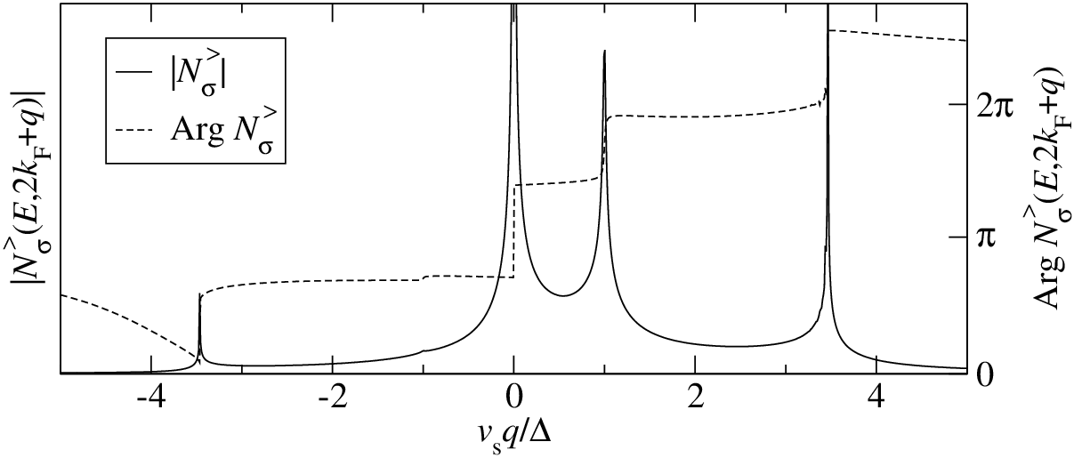
In Figs. 1 and 2 we plot Nσ>​(E,2​kF+q)N^{>}_{\sigma}(E,2k_{\mathrm{F}}+q) for the case of unbroken spin rotational symmetry (Ks=1K_{\mathrm{s}}=1). The Fourier transform of the LDOS is dominated by a singularity at momentum 2​kF2k_{\mathrm{F}} (q=0q=0), which arises from the contribution N1>N^{>}_{1}. For fixed energy and close to the singularity this term behaves as (see App. F)

N1>​(E,2​kF+q)∼(1vc​q)α,α=1−Kc22,N^{>}_{1}(E,2k_{\mathrm{F}}+q)\sim\left(\frac{1}{v_{\mathrm{c}}q}\right)^{\alpha},\quad\alpha=1-\frac{K_{\mathrm{c}}^{2}}{2}, (29)

which implies a phase jump of π​α\pi\alpha as q→0±q\rightarrow 0\pm. This peak is indicative of the CDW order being pinned at the boundary. We note, however, that the peak occurs at finite energies and hence the underlying process is not static. A similar feature can be seen in the Luttinger liquid case [9], where the singularity as a function of qq is softer (αLL=(1−Kc2)/2\alpha_{\mathrm{LL}}=(1-K_{\mathrm{c}}^{2})/2).

At low energies above the spin gap Δ\Delta we further observe two dispersing features associated with the collective spin and charge degrees of freedom respectively. These are broadly similar to the bulk single-particle spectral function [50, 51] and feature (1) a “charge peak” that follows

Ec​(q)=vc​|q|2+ΔE_{\mathrm{c}}(q)=\frac{v_{\mathrm{c}}|q|}{2}+\Delta (30)

and (2) a “spin peak” at position

Es​(q)=(vs​q2)2+Δ2.E_{\mathrm{s}}(q)=\sqrt{\left(\frac{v_{\mathrm{s}}q}{2}\right)^{2}+\Delta^{2}}. (31)

We note that neither peak is sharp (i.e. they are not delta-functions) and hence have to be thought of as arising from excitations involving at least two “elementary” constituents. In this way of thinking, the charge peak arises from two-particle excitations composed of a “zero momentum” spinon contributing an energy Δ\Delta and a gapless antiholon of “momentum” qq. On the other hand, the spin peak can be thought of arising from two-particle excitations composed of a “zero momentum” antiholon and a spinon of “momentum” qq. The appearance of vc/2v_{\mathrm{c}}/2 and vs/2v_{\mathrm{s}}/2 in (30) and (31), respectively, is due to the fact that the particles have to propagate to the boundary and back, thus covering the distance 2​x2x in time tt. We note that on a technical level the charge peak arises from the contribution N1>N^{>}_{1} to the Fourier transform of the LDOS, whereas the spin peak has its origin in N2>N^{>}_{2}, which encodes the effects of the boundary on the spin degrees of freedom. In the q<0q<0 region the dispersing features are strongly suppressed and for Kc=1K_{\mathrm{c}}=1 the charge feature is found to vanish entirely.

It is instructive to plot Nσ>​(E,2​kF+q)N^{>}_{\sigma}(E,2k_{\mathrm{F}}+q) as a function of qq for fixed energy, see Fig. 2. We observe characteristic jumps in the phase Arg​Nσ>\text{Arg}\,N^{>}_{\sigma} at the peak positions. This is similar to the Luttinger liquid case [9].
Refer to caption
Figure 2: Constant energy scan for E=2​ΔE=2\Delta: |Nσ>​(E,2​kF+q)||N^{>}_{\sigma}(E,2k_{\mathrm{F}}+q)| (arbitrary units) and Arg​Nσ>​(E,2​kF+q)\text{Arg}N^{>}_{\sigma}(E,2k_{\mathrm{F}}+q) for Kc=0.8K_{\mathrm{c}}=0.8, Ks=1K_{\mathrm{s}}=1 and vc=2​vsv_{\mathrm{c}}=2v_{\mathrm{s}}. We observe a peak at q=0q=0 (related to the pinning of the CDW at the boundary) and dispersing features at q=±2(E−Δ)/vcq=\pm 2(E-\Delta)/v_{\mathrm{c}} as well as q=±2E2−Δ2/vsq=\pm 2\sqrt{E^{2}-\Delta^{2}}/v_{\mathrm{s}}. For q<0q<0 the dispersing features are strongly suppressed. Furthermore, we observe characteristic jumps in the argument at the positions of the peaks.

IV.2 Attractive case

We now turn to the case of a CDW state arising in a system with (effective) attractive electron-electron interactions. As discussed in Sec. II, this case arises in electron-phonon systems. The effective parameters are given by vs>vcv_{\mathrm{s}}>v_{\mathrm{c}} and Kc>1>KsK_{\mathrm{c}}>1>K_{\mathrm{s}}.

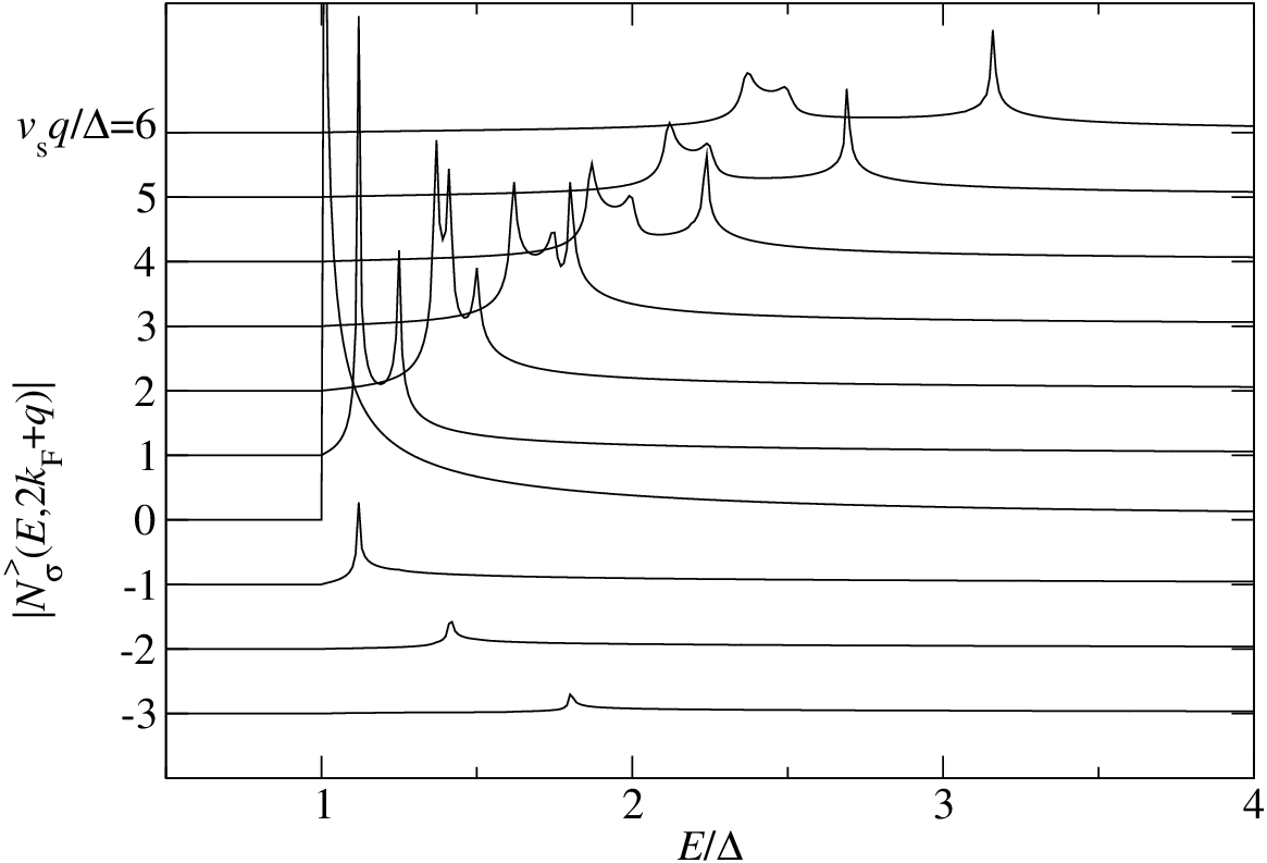
In Fig. 3 we plot Nσ>​(E,2​kF+q)N^{>}_{\sigma}(E,2k_{\mathrm{F}}+q) as a function of energy for several values of qq (in units of the spin gap). We again observe a singularity at 2​kF2k_{\mathrm{F}}, which arises from (29). The singularity is much less pronounced than in the repulsive case and disappears for Kc≥2K_{\mathrm{c}}\geq\sqrt{2}. Like in the repulsive case there are several dispersing features:

  1. 1.

    a charge peak at E=Ec​(q)E=E_{\mathrm{c}}(q), where EcE_{\mathrm{c}} is given by (30);

  2. 2.

    a spin peak at E=Es​(q)E=E_{\mathrm{s}}(q), where EsE_{\mathrm{s}} is defined in (31);

  3. 3.

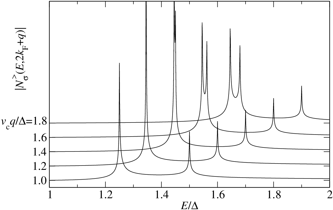
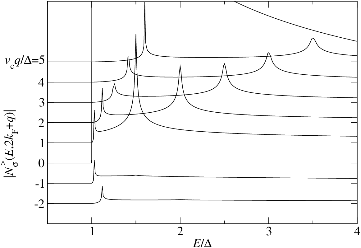
    when |q||q| exceeds a critical value q0q_{0} a third dispersing low-energy peak appears (see Fig. 4) at

    Ecs​(q)=vc​|q|2+Δ​1−(vcvs)2=Es​(q0)+vc2​(|q|−q0),q0=2​Δ​vcvs​vs2−vc2.E_{\mathrm{cs}}(q)=\frac{v_{\mathrm{c}}|q|}{2}+\Delta\sqrt{1-\left(\frac{v_{\mathrm{c}}}{v_{\mathrm{s}}}\right)^{2}}=E_{\mathrm{s}}(q_{0})+\frac{v_{\mathrm{c}}}{2}\bigl(|q|-q_{0}\bigr),\quad q_{0}=\frac{2\Delta v_{\mathrm{c}}}{v_{\mathrm{s}}\sqrt{v_{\mathrm{s}}^{2}-v_{\mathrm{c}}^{2}}}. (32)

    This feature can be thought of as arising from a “momentum” q0q_{0} spinon and an antiholon carrying “momentum” q−q0q-q_{0}. We note that in this case the spin and charge excitations have the same group velocity

    ∂Ec∂q=∂Es∂q|q=q0=vc2.\frac{\partial E_{\mathrm{c}}}{\partial q}=\frac{\partial E_{\mathrm{s}}}{\partial q}\bigg|_{q=q_{0}}=\frac{v_{\mathrm{c}}}{2}. (33)

This behavior is reminiscent of what is found for the single-particle spectral function in the bulk [50, 51]. The peak splitting and hence the qualitative difference between the repulsive and attractive regime is a consequence of the curvature of the (anti)soliton dispersion relation and hence of the spin gap. In the Luttinger liquid case [9] (where both sectors are massless) there are only two dispersing features in both regimes.
Refer to caption
Figure 3: |Nσ>​(E,2​kF+q)||N^{>}_{\sigma}(E,2k_{\mathrm{F}}+q)| (arbitrary units) for Kc=1.2K_{\mathrm{c}}=1.2, Ks=1K_{\mathrm{s}}=1 and vs=2​vcv_{\mathrm{s}}=2v_{\mathrm{c}}. The curves are constant qq-scans which have been offset along the y-axis by a constant with respect to one another. The peak at q=0q=0 is much less pronounced then in the repulsive case (see Fig. 1). We observe dispersing features at EcE_{\mathrm{c}}, EsE_{\mathrm{s}}, and Ecs=vc​|q|/2+Δ​1−(vc/vs)2E_{\mathrm{cs}}=v_{\mathrm{c}}|q|/2+\Delta\sqrt{1-(v_{\mathrm{c}}/v_{\mathrm{s}})^{2}} (for |q|>q0|q|>q_{0} only).
Refer to caption
Figure 4: |Nσ>​(E,2​kF+q)||N^{>}_{\sigma}(E,2k_{\mathrm{F}}+q)| (arbitrary units) for Kc=1K_{\mathrm{c}}=1, Ks=1/2K_{\mathrm{s}}=1/\sqrt{2}, vs=1.5​vcv_{\mathrm{s}}=1.5\,v_{\mathrm{c}}, δ=0.001\delta=0.001, and vc​q/Δ=1.0,…,1.8v_{\mathrm{c}}q/\Delta=1.0,\ldots,1.8. The curves have been offset along the y-axis by a constant with respect to one another. We observe the splitting of the spin peak at EsE_{\mathrm{s}} at the critical momentum vc​q0/Δ≈1.19v_{\mathrm{c}}q_{0}/\Delta\approx 1.19.

IV.3 Higher-order corrections

As we have indicated in Eq. (20) there are contributions to the LDOS beyond those that we have discussed above. They arise from our calculation of the spin-part of the Green function and are expected to be small[48]. In order to verify that they can indeed be neglected, we have analyzed them in some detail at the LEP Ks=1/2K_{\mathrm{s}}=1/\sqrt{2}, where the necessary matrix elements take a particularly simple form, which makes the actual calculations much easier.

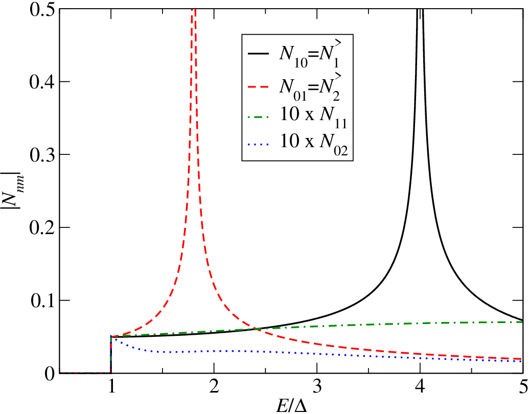
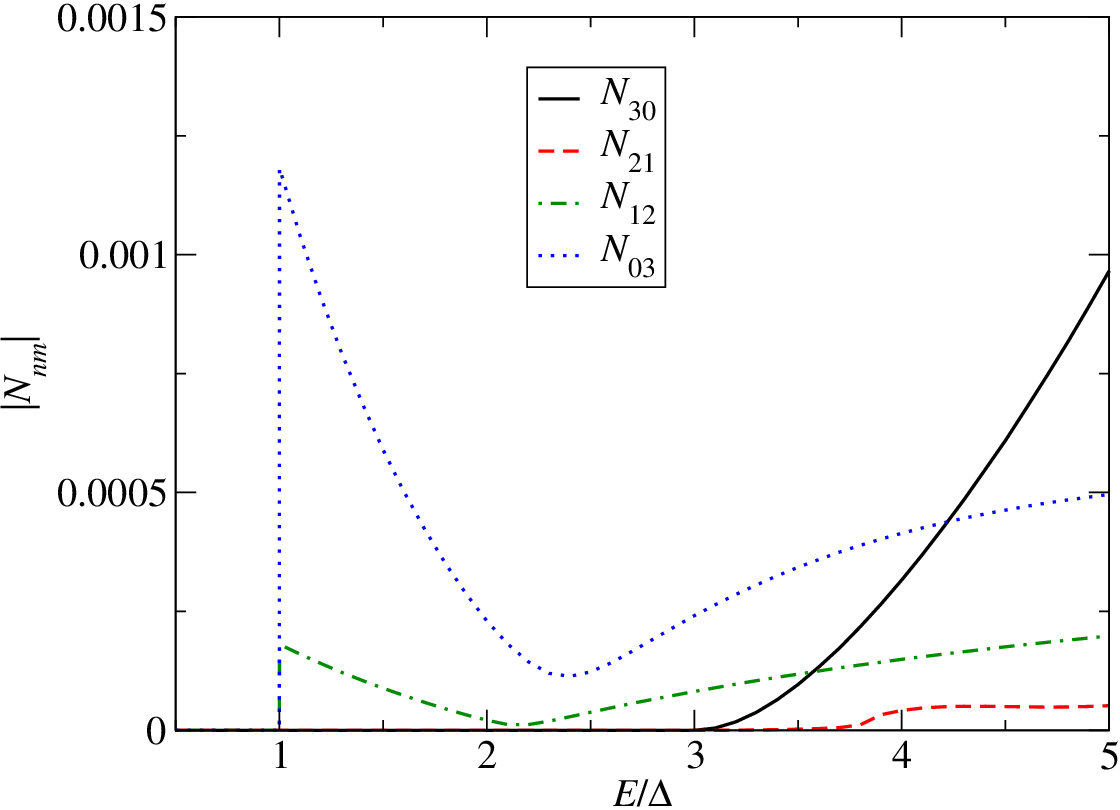
Our purpose is then to determine further terms in the the expansion (26) of Nσ>​(E,2​kF+q)N^{>}_{\sigma}(E,2k_{\mathrm{F}}+q). We denote by Nn​mN_{nm} the contribution to (26) that arises from processes in which nn gapped spinons (which correspond to solitons/antisolitons in the sine-Gordon model describing the spin sector) propagate between (0,x2)(0,x_{2}) and (τ,x1)(\tau,x_{1}), and which involves the mm’th power of the boundary reflection matrix KK. The terms discussed above correspond to N10=N1>N_{10}=N^{>}_{1} and N01=N2>N_{01}=N^{>}_{2}. In App. C.4 we present some details on the calculation of the terms in the form-factor expansion of gs​(τ,x1,x2)g_{s}(\tau,x_{1},x_{2}) that give rise to Nn​mN_{nm} with m+n≤3m+n\leq 3. The number of θ\theta-integrations in Nn​mN_{nm} equals m+nm+n (cf. (27)). We find that their contributions to the Fourier transform of the LDOS are small. In particular, all qualitative features of the LDOS such as dispersing peaks are already encoded in N10N_{10} and N01N_{01}.

Refer to caption
Refer to caption
Figure 5: (Color online) Left: Comparison of the absolute values of N10=N1>​(E,2​kF+q)N_{10}=N^{>}_{1}(E,2k_{\mathrm{F}}+q) and N01=N2>​(E,2​kF+q)N_{01}=N^{>}_{2}(E,2k_{\mathrm{F}}+q) to the sub-leading terms N11N_{11} and N02N_{02} (N20=0N_{20}=0). We stress that the scale for the higher-order terms has been magnified. Right: Absolute values of the terms N30N_{30}, N21N_{21}, N12N_{12}, and N03N_{03}. We stress the different scales on the y-axis. The parameters are Kc=1K_{\mathrm{c}}=1, Ks=1/2K_{\mathrm{s}}=1/\sqrt{2}, vc=2​vsv_{\mathrm{c}}=2v_{\mathrm{s}}, and vs​q/Δ=3v_{\mathrm{s}}q/\Delta=3. The three-particle contributions N30N_{30} and N21N_{21} vanish for E<3​ΔE<3\Delta. Furthermore, the higher-order terms possess no peaks.

In Fig. 5 we show the leading terms N10N_{10} and N01N_{01} as well as the sub-leading terms for Kc=1K_{\mathrm{c}}=1 and vc>vsv_{\mathrm{c}}>v_{\mathrm{s}} for a fixed value of qq as a function of energy. We see that the two leading terms in (26) indeed capture all qualitative features of the LDOS and carry the main part of the spectral weight at low energies E≤5​ΔE\leq 5\Delta. The higher-order terms are small compared to N10N_{10} and N01N_{01}. In particular, N30N_{30} vanishes for E<3​ΔE<3\Delta, since this term originates from a three-particle process. In general, all terms Nn​mN_{nm} originating from nn-particle processes vanish for E<n​ΔE<n\Delta. Most importantly, however, the higher-order terms do not possess any singularities. The suppression of subleading terms in the form-factor expansion for bulk two-point functions is a well-known feature of massive theories [52, 53, 44], whereas the smallness of terms involving higher powers of the boundary reflection amplitude KK has recently been demonstrated for the Ising model with a boundary magnetic field [48].

IV.4 Small-momentum regime

The small-momentum regime Q≈0Q\approx 0 of the Fourier transform of the LDOS can be analyzed in the same way as in the Q≈2​kFQ\approx 2k_{\mathrm{F}} case discussed above. We note that the LDOS for Q≈0Q\approx 0 is non-vanishing even in absence of a boundary [50, 51]. In the presence of a boundary the Fourier transform of the LDOS for Q≈0Q\approx 0 is obtained from (23). The leading terms are given by Nσ>​(E,Q)=∑i=12Ni>​(E,Q)+…N^{>}_{\sigma}(E,Q)=\sum_{i=1}^{2}N^{>}_{i}(E,Q)+\ldots, where

Ni>​(E,Q)\displaystyle N^{>}_{i}(E,Q) =\displaystyle= −Θ⁡(E−Δ)​Z1​e−i​π2​(2​c+1)​Γ​(a+b+1)4​π2​vca+b−1​Γ​(2​a+2​b)\displaystyle-\Theta(E-\Delta)\,\frac{Z_{1}\,e^{-\text{i}\frac{\pi}{2}(2c+1)}\,\Gamma(a+b+1)}{4\pi^{2}\,v_{\mathrm{c}}^{a+b-1}\,\Gamma(2a+2b)} (34)
×∫−AAd​θ​hi​(θ)​ui2​c+1(E−Δ​cosh⁡θ)2−a−b​F1​(a+b+1,c,c,2​a+2​b,ui∗,−ui).\displaystyle\qquad\times\int_{-A}^{A}d\theta\frac{h_{i}(\theta)\,u_{i}^{2c+1}}{(E\!-\!\Delta\cosh\theta)^{2-a-b}}\,F_{1}\bigl(a+b+1,c,c,2a+2b;u_{i}^{*},-u_{i}\bigr).

Here we have |Q|≪kF|Q|\ll k_{\mathrm{F}}, A=arcosh⁡(EΔ)A=\mathrm{arcosh}\bigl(\tfrac{E}{\Delta}\bigr), h1​(θ)=eθ/2h_{1}(\theta)=e^{\theta/2}, h2​(θ)=K⁡(θ+i​π2)h_{2}(\theta)=K\bigl(\theta+\text{i}\tfrac{\pi}{2}\bigr), and u1,2u_{1,2} are defined in (28) with qq replaced by QQ. The main difference to (26) is in the dependence of Appell’s hypergeometric function on KcK_{\mathrm{c}}.

Refer to caption
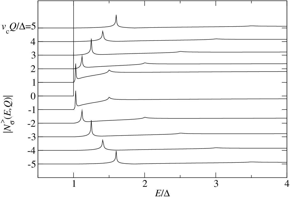
Figure 6: |Nσ>​(E,Q)||N^{>}_{\sigma}(E,Q)| (arbitrary units) for Kc=0.8K_{\mathrm{c}}=0.8, Ks=1K_{\mathrm{s}}=1 and vc=2​vsv_{\mathrm{c}}=2v_{\mathrm{s}}. The curves are constant QQ-scans which have been offset along the y-axis by a constant with respect to one another. We observe dispersing features at Ec​(Q)E_{\mathrm{c}}(Q) and Es​(Q)E_{\mathrm{s}}(Q). The charge features are very weak for all momenta. We further observe a constant background at energies larger than the spin gap.

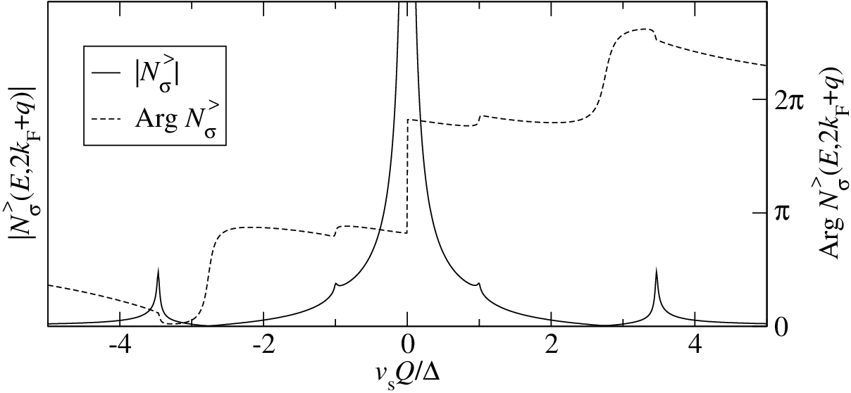
In Figs. 6 and 7 we plot Nσ>​(E,Q)N^{>}_{\sigma}(E,Q) for the case of repulsive electron interactions and unbroken spin rotational symmetry. It is dominated by a singularity at Q=0Q=0, which has its origin in N1>N_{1}^{>} and behaves as ∼1/Q\sim 1/Q independently of KcK_{\mathrm{c}}. This singularity is more pronounced than its counterpart at 2​kF2k_{\mathrm{F}}. We further observe dispersing features at positions Ec​(Q)E_{\mathrm{c}}(Q) and Es​(Q)E_{\mathrm{s}}(Q) respectively. Both of these are symmetric under Q→−QQ\rightarrow-Q. The peak at Ec​(Q)E_{\mathrm{c}}(Q) is strongly suppressed, vanishes for Kc=1K_{\mathrm{c}}=1, and becomes a dip in the attractive regime. The suppression is due to the softness of the singularities of GR​RG^{RR} at vc​t=2​Rv_{\mathrm{c}}t=2R. On the other hand, the charge part of (23) has its strongest singularity at vc​t=r=0v_{\mathrm{c}}t=r=0, which results in a background of spectral weight in Nσ>​(E,Q)N^{>}_{\sigma}(E,Q) for all energies above the spin gap.

In the attractive case (vs>vcv_{\mathrm{s}}>v_{\mathrm{c}}) we observe a peak-splitting similiar to that in the 2​kF2k_{\mathrm{F}}-component, but all peaks are very weak.
Refer to caption
Figure 7: Constant energy scan for E=2​ΔE=2\Delta: |Nσ>​(E,Q)||N^{>}_{\sigma}(E,Q)| (arbitrary units) and Arg​Nσ>​(E,Q)\text{Arg}N^{>}_{\sigma}(E,Q) for Kc=0.8K_{\mathrm{c}}=0.8, Ks=1K_{\mathrm{s}}=1 and vc=2​vsv_{\mathrm{c}}=2v_{\mathrm{s}}. We observe a strong peak at Q=0Q=0 and dispersing features at Q=±2(E−Δ)/vcQ=\pm 2(E-\Delta)/v_{\mathrm{c}} as well as Q=±2E2−Δ2/vsQ=\pm 2\sqrt{E^{2}-\Delta^{2}}/v_{\mathrm{s}}. Note that |Nσ>​(E,Q)||N^{>}_{\sigma}(E,Q)| is symmetric under Q→−QQ\rightarrow-Q.

V General boundary conditions and boundary bound states

So far we have considered the simplest possible boundary conditions corresponding to a spin-independent phase shift of π\pi. Both ways of realizing a boundary in a (quasi) one dimension system that we have discussed above (i.e. as a result of an impurity or in a “two-tip” STS experiment) are expected to give rise to a local potential or magnetic field. These correspond to more general phase shifts for reflection of particles at the boundary. As is well known, such more general boundary conditions can give rise to boundary bound states, see for example Refs. [54]. These are expected to be visible in the Fourier transform of the LDOS as “resonances” inside the single-particle gap. This is most easily seen by considering a Lehmann representation of Nσ>​(E,Q)N^{>}_{\sigma}(E,Q) in terms of the eigenstates |nb⟩|n_{\mathrm{b}}\rangle on the half-line

Nσ>(E,Q)=∫−∞0dxe−i​Q​x∑nb|⟨0b|Ψσ(0,x)|nb⟩|2δ(E−Enb).N^{>}_{\sigma}(E,Q)=\int_{-\infty}^{0}dx\,e^{-\text{i}Qx}\,\sum_{n_{\mathrm{b}}}\,\big|\!\left\langle 0_{\mathrm{b}}\right|\Psi_{\sigma}(0,x)\left|n_{\mathrm{b}}\right\rangle\big|^{2}\,\delta(E-E_{n_{\mathrm{b}}}). (35)

For boundary bound states |bbs,α⟩|{\rm bbs},\alpha\rangle we have 0<Ebbs,α<Δ0<E_{{\rm bbs},\alpha}<\Delta, which leads to features in Nσ>​(E,Q)N^{>}_{\sigma}(E,Q) below the single-particle gap. As we are dealing with a spin-charge separated system, these features will generally not be sharp as the bound state occurs only in the gapped sector of the theory. We now turn to calculating the LDOS in cases where boundary bound states exist. We first consider boundary conditions of the form

Rσ(τ,0)=−e−ifσΦs0/2Lσ(τ,0),R_{\sigma}(\tau,0)=-e^{-\text{i}f_{\sigma}\Phi_{\mathrm{s}}^{0}/2}\,L_{\sigma}(\tau,0), (36)

where f↑=1=−f↓f_{\uparrow}=1=-f_{\downarrow}. In terms of the Bose fields these boundary conditions read

Φc​(τ,0)=0,Φs​(τ,0)=Φs0,0≤Φs0<π.\Phi_{\mathrm{c}}(\tau,0)=0,\qquad\Phi_{\mathrm{s}}(\tau,0)=\Phi_{\mathrm{s}}^{0},\quad 0\leq\Phi_{\mathrm{s}}^{0}<\pi. (37)

We note that these boundary conditions break spin rotational symmetry. However, if we go over to the case of a one-dimensional Mott insulator by exchanging spin and charge degrees of freedom, the spin rotational symmetry remains intact and the boundary conditions correspond to a local potential.

As before we will focus on the 2​kF2k_{\mathrm{F}}-component of the Fourier transform of the LDOS. As we have changed the boundary conditions only in the spin sector, the charge part (19) of the chiral Green function remains unchanged.

The two leading terms of the form-factor expansion in the spin sector are still of the form (20), but now the boundary reflection amplitude KK is different and in particular is spin-dependent. At the LEP it is given by [45]

Kσ​σ¯​(θ)=sin⁡(i​θ2−fσ​Φs02)cos⁡(i​θ2+fσ​Φs02),Kσ​σ​(θ)=Kσ¯​σ¯​(θ)=0.K^{\sigma\bar{\sigma}}(\theta)=\frac{\sin\Bigl(\text{i}\frac{\theta}{2}-f_{\sigma}\frac{\Phi_{\mathrm{s}}^{0}}{2}\Bigr)}{\cos\Bigl(\text{i}\frac{\theta}{2}+f_{\sigma}\frac{\Phi_{\mathrm{s}}^{0}}{2}\Bigr)},\quad K^{\sigma\sigma}(\theta)=K^{\bar{\sigma}\bar{\sigma}}(\theta)=0. (38)

Here we have introduced the notations ↑=+\uparrow=+ and ↓=−\downarrow=- as well as σ¯=−\bar{\sigma}=- for σ=+\sigma=+ and vice versa. We note that as a result of a different choice of phase for the asymptotic states Eq. (38) differs by a minus sign from Ref. [45] (see also App. C). The expressions for general KsK_{\mathrm{s}} can be found in Refs. [29, 46, 47].

In the spin rotationally symmetric case Ks=1K_{\mathrm{s}}=1 we have K+⁣−​(θ)=K−⁣+​(θ)=K⁡(θ)K^{+-}(\theta)=K^{-+}(\theta)=K(\theta), where K⁡(θ)K(\theta) is given in (21). We stress that the Green function remains diagonal in spin space, Gσ​σ′R​L∝δσ​σ′G^{RL}_{\sigma\sigma^{\prime}}\propto\delta_{\sigma\sigma^{\prime}}, and that the spin-dependence is entirely due to the boundary reflection matrix Kσ​σ¯K^{\sigma\bar{\sigma}}. Before presenting the resulting LDOS we discuss the emergence of a boundary bound state in the spin sector [29, 55, 46]. If we choose the phase-shift Φs0\Phi_{\mathrm{s}}^{0} in the spin sector such that

Ks2​π<Φs0,K_{\mathrm{s}}^{2}\pi<\Phi_{\mathrm{s}}^{0}, (39)

the boundary reflection amplitude K−⁣+​(θ)K^{-+}(\theta) has a pole in the physical strip 0≤ℑ​𝔪​θ≤π/20\leq\mathfrak{Im}\,\theta\leq\pi/2. This pole corresponds to a boundary bound state with energy

Ebbs=Δ​sin⁡γ,γ=π−Φs02−2​Ks2.E_{\mathrm{bbs}}=\Delta\,\sin\gamma,\quad\gamma=\frac{\pi-\Phi_{\mathrm{s}}^{0}}{2-2K_{\mathrm{s}}^{2}}. (40)

The physical nature of the bound state has been discussed by Ghoshal and Zamolodchikov [29]. The classical ground state of the sine-Gordon model on the half-line (14) in the entire range 0≤Φs0<π0\leq\Phi_{\mathrm{s}}^{0}<\pi is characterized by the asymptotic behavior Φs→0\Phi_{\mathrm{s}}\rightarrow 0 as x→−∞x\rightarrow-\infty. On the other hand, there exists a second classically stable state satisfying Φs→2​π\Phi_{\mathrm{s}}\rightarrow 2\pi as x→−∞x\rightarrow-\infty. When Φs0\Phi_{\mathrm{s}}^{0} is sufficiently large this state is expected to be stable in the quantum theory as well.

We note that for Φs0=π\Phi_{\mathrm{s}}^{0}=\pi both states are degenerate and (40) vanishes. In the attractive regime of the sine-Gordon model Ks<1/2K_{\mathrm{s}}<1/\sqrt{2} additional boundary bound states occur, while in the spin rotationally invariant case Ks→1K_{\mathrm{s}}\rightarrow 1 the condition Ks2​π<Φs0<πK_{\mathrm{s}}^{2}\pi<\Phi_{\mathrm{s}}^{0}<\pi is never satisfied and hence no boundary bound states exist.

When calculating dynamical response functions in the boundary state formalism additional contributions in the form factor expansions occur upon analytical continuation in the rapidity variables. In particular, the pole of the boundary reflection amplitude in the physical strip gives rise to an additional term linear in KK in the form-factor expansion (20). In the case τ>0\tau>0 and x1<x2x_{1}<x_{2} it takes the form (see App. C.5)

Θ⁡(Φs0−Ks2​π)​δσ↓​Z1​B​ei2​γ​e2​Δvs​R​cos⁡γ​e−Δ​τ​sin⁡γ,\Theta\Bigl(\Phi_{\mathrm{s}}^{0}-K_{\mathrm{s}}^{2}\,\pi\Bigr)\,\delta_{\sigma\downarrow}\,Z_{1}\,B\,e^{\frac{\text{i}}{2}\gamma}\,e^{2\frac{\Delta}{v_{\mathrm{s}}}R\cos\gamma}\,e^{-\Delta\tau\sin\gamma}, (41)

where the constant B≥0B\geq 0 is related to the residue of K∓⁣±​(θ)K^{\mp\pm}(\theta) (see (108)). At the LEP it equals B=−2cosΦs0B=-2\cos\Phi_{\mathrm{s}}^{0}. We stress that this additional term appears in the down-spin channel only, since we have assumed 0≤Φs0<π0\leq\Phi_{\mathrm{s}}^{0}<\pi. If we were to consider −π<Φs0≤0-\pi<\Phi_{\mathrm{s}}^{0}\leq 0, we would find a term similar to (41) in the up-spin channel only.

The Fourier transform of the LDOS for the boundary conditions (37) can be expanded as before and is expressed as

Nσ>​(E,2​kF+q)=∑i=13Nσ,i>​(E,2​kF+q)+….N^{>}_{\sigma}(E,2k_{\mathrm{F}}+q)=\sum_{i=1}^{3}N^{>}_{\sigma,i}(E,2k_{\mathrm{F}}+q)+\ldots. (42)

Here the first two terms are again of the form (27), where in the second term Nσ,2>N^{>}_{\sigma,2} we need to replace the boundary reflection amplitude K⁡(θ+i​π2)K\bigl(\theta+\text{i}\frac{\pi}{2}\bigr) by its spin-dependent counterpart Kσ​σ¯​(θ+i​π2)K^{\sigma\bar{\sigma}}\bigl(\theta+\text{i}\frac{\pi}{2}\bigr). The third term is obtained from (41) and arises as a result of the presence of a boundary bound state. Explicitly it reads

Nσ,3>​(E,2​kF+q)\displaystyle N^{>}_{\sigma,3}(E,2k_{\mathrm{F}}+q) =\displaystyle= Θ⁡(Φs0−Ks2​π)​Θ​(E−Ebbs)​δσ↓​Z1​B4​π​Γ⁡(2​c+1)Γ⁡(a+b+2​c)​i​ei2​γ​e−i​π​cvca+b−1\displaystyle\Theta\Bigl(\Phi_{\mathrm{s}}^{0}-K_{\mathrm{s}}^{2}\,\pi\Bigr)\,\Theta\Bigl(E-E_{\mathrm{bbs}}\Bigr)\,\delta_{\sigma\downarrow}\,\frac{Z_{1}B}{4\pi}\,\frac{\Gamma(2c+1)}{\Gamma(a+b+2c)}\,\frac{\text{i}\,e^{\frac{\text{i}}{2}\gamma}\,e^{-\text{i}\pi c}}{v_{\mathrm{c}}^{a+b-1}} (43)
×(2vc​q​(E−Ebbs)+i​sgn​(vs​qΔ)​δ)2​c+1(E−Ebbs)2−a−b​FD(3)​(2​c+1,a,b,2​c,a+b+2​c,u3∗,−u3,−u3′).\displaystyle\times\frac{\left(\frac{2}{v_{\mathrm{c}}q}(E-E_{\mathrm{bbs}})+\text{i}\,\text{sgn}(\frac{v_{\mathrm{s}}q}{\Delta})\,\delta\right)^{2c+1}}{\bigl(E-E_{\mathrm{bbs}}\bigr)^{2-a-b}}\,F_{\mathrm{D}}^{(3)}\bigl(2c+1,a,b,2c,a+b+2c;u_{3}^{*},-u_{3},-u_{3}^{\prime}\bigr).

Here FD(3)F_{\mathrm{D}}^{(3)} denotes Lauricella’s hypergeometric function of three arguments [56] (see App. E) and

u3=2vc​q​(E−Ebbs)+i​2​Δvs​q​cos⁡γ,u3′=i​2​Δvs​q​cos⁡γ,u_{3}=\frac{2}{v_{\mathrm{c}}q}(E-E_{\mathrm{bbs}})+\text{i}\frac{2\Delta}{v_{\mathrm{s}}q}\cos\gamma,\quad u_{3}^{\prime}=\text{i}\frac{2\Delta}{v_{\mathrm{s}}q}\cos\gamma, (44)

where the constant γ\gamma defined in (40). The Fourier transform of the LDOS (42) has a non-dispersing singularity at its lower threshold

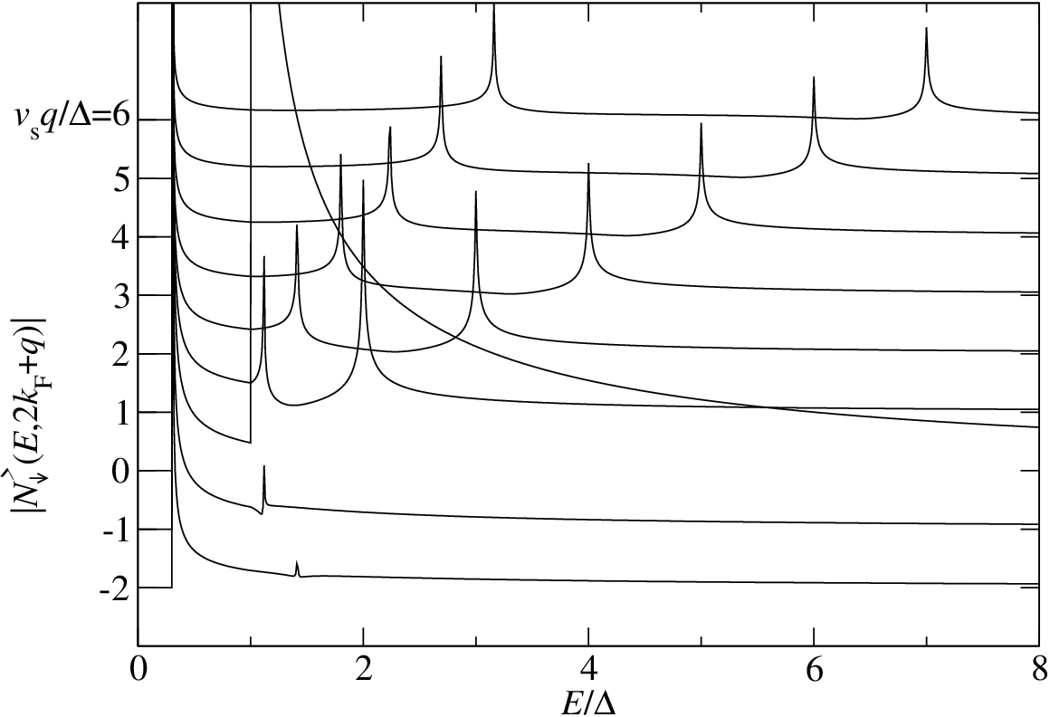
Nσ,3>​(E,2​kF+q)∝δσ↓(E−Ebbs)α,α=1−12​Kc2.N^{>}_{\sigma,3}(E,2k_{\mathrm{F}}+q)\propto\frac{\delta_{\sigma\downarrow}}{(E-E_{\mathrm{bbs}})^{\alpha}},\quad\alpha=1-\frac{1}{2K_{\mathrm{c}}^{2}}. (45)

The emergence of a non-dispersing feature within the spin gap signals the presence of a boundary bound state. In Fourier space the LDOS is a convolution of contributions from the spin and charge sectors. As we are dealing with a bound state in the spin sector, the exponent of the singularity depends only on the Luttinger parameter in the charge sector. We note that the singularity occurs only in the down-spin channel and disappears for Kc2≤1/2K_{\mathrm{c}}^{2}\leq 1/2. On the other hand, in Nσ<N^{<}_{\sigma} the additional feature due to the boundary bound state appears only in the up-spin channel.
Refer to caption
Figure 8: |N↓>​(E,2​kF+q)||N^{>}_{\downarrow}(E,2k_{\mathrm{F}}+q)| (arbitrary units) for Kc=1K_{\mathrm{c}}=1, Ks=1/2K_{\mathrm{s}}=1/\sqrt{2}, vc=2​vsv_{\mathrm{c}}=2v_{\mathrm{s}}, and Φs0=0.9​π\Phi_{\mathrm{s}}^{0}=0.9\pi. The curves are constant qq-scans which have been offset along the y-axis by a constant with respect to one another. We observe dispersing features at Es​(q)E_{\mathrm{s}}(q) and Ec​(q)E_{\mathrm{c}}(q) (for q>0q>0 only) as well as a non-dispersing singularity at E=EbbsE=E_{\mathrm{bbs}}, which is due to the formation of a boundary bound state in the spin sector.

In Fig. 8 we plot the down-spin component of (42) for vc>vsv_{\mathrm{c}}>v_{\mathrm{s}} as a function of energy for several values of qq. As before, at low energies above the spin gap Δ\Delta we observe two dispersing features associated with the collective spin and charge degrees of freedom that follow EsE_{\mathrm{s}} and EcE_{\mathrm{c}} respectively. In addition, we observe the non-dispersing singularity (45) at E=EbbsE=E_{\mathrm{bbs}}.

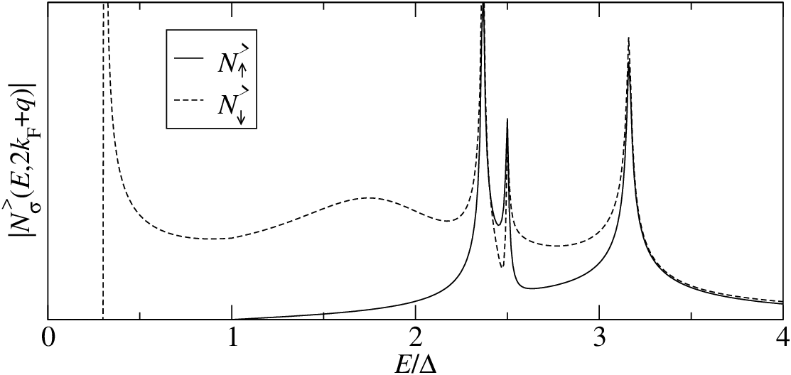
In Fig. 9 we plot N↑>N^{>}_{\uparrow} and N↓>N^{>}_{\downarrow} as functions of energy for vc<vsv_{\mathrm{c}}<v_{\mathrm{s}}. We see that the singularity arising due to the presence of a boundary bound state appears only in the down-spin channel. For either spin polarization we observe three dispersing features at Ec​(q)E_{\mathrm{c}}(q), Es​(q)E_{\mathrm{s}}(q) and Ecs​(q)E_{\mathrm{cs}}(q) respectively. Their interpretations are completely analogous to discussion in Sec. IV.2. In addition to these sharp peaks we observe a broad maximum in the down-spin channel at energies E≈Ebbs+vc​q/2E\approx E_{\mathrm{bbs}}+v_{\mathrm{c}}q/2. This feature is suppressed for vc>vsv_{\mathrm{c}}>v_{\mathrm{s}}, see Fig. 8. Its physical origin is the simultaneous excitation of the boundary bound state and a finite energy excitation in the charge sector. We note that the asymmetry in N↑>​(E,Q)−N↓>​(E,Q)N^{>}_{\uparrow}(E,Q)-N^{>}_{\downarrow}(E,Q) could in principle be detected in experiments using a magnetic STM tip.
Refer to caption
Figure 9: |N↑>​(E,2​kF+q)||N^{>}_{\uparrow}(E,2k_{\mathrm{F}}+q)| (full line) and |N↓>​(E,2​kF+q)||N^{>}_{\downarrow}(E,2k_{\mathrm{F}}+q)| (dashed line) for vs​q/Δ=6v_{\mathrm{s}}q/\Delta=6, Kc=1K_{\mathrm{c}}=1, Ks=1/2K_{\mathrm{s}}=1/\sqrt{2}, vs=2​vcv_{\mathrm{s}}=2v_{\mathrm{c}}, and Φs0=0.9​π\Phi_{\mathrm{s}}^{0}=0.9\,\pi. The broad maximum at E≈1.8E\approx 1.8 is caused by the excitation of the boundary bound state and additional charge excitations.

So far we have considered only hard-wall boundary conditions in the charge sector, i.e. Φc​(x=0)=0\Phi_{\mathrm{c}}(x=0)=0. Our analysis can be straightforwardly extended to the case Φc​(x=0)=Φc0\Phi_{\mathrm{c}}(x=0)=\Phi_{\mathrm{c}}^{0}, which in terms of the original electrons corresponds to a local potential close to the boundary.

VI Finite-temperature LDOS

Another interesting issue concerns the effects of a finite temperature on the LDOS. The regime T≲Δ/2T\lesssim\Delta/2 can in principle be analyzed by generalizing the methods recently developed in Refs. [57] to the boundary state formalism. However, in order to keep matters simple we will restrict ourselves to the regime of very low temperatures T≪ΔT\ll\Delta. Here the main effects arise from a modification of the dynamical response in the gapless charge sector and correlation functions in the spin sector can be approximated by their T=0T=0 expressions. This is the case because we only consider response functions that involve both sectors. The charge part of the Green function Gσ​σ′R​L​(τ,x1,x2)=gc​(τ,x1,x2)​gs​(τ,x1,x2)G^{RL}_{\sigma\sigma^{\prime}}(\tau,x_{1},x_{2})=g_{\mathrm{c}}(\tau,x_{1},x_{2})\,g_{\mathrm{s}}(\tau,x_{1},x_{2}) can be evaluated using conformal field theory methods [58, 38] and is found to be

gc​(τ,x1,x2)\displaystyle g_{\mathrm{c}}(\tau,x_{1},x_{2}) =\displaystyle= −δσ​σ′2​π​(πvc​β)a+b​1sina⁡(πvc​β​(vc​τ−2​i​R))​1sinb⁡(πvc​β​(vc​τ+2​i​R))\displaystyle-\frac{\delta_{\sigma\sigma^{\prime}}}{2\pi}\left(\frac{\pi}{v_{\mathrm{c}}\beta}\right)^{a+b}\frac{1}{\sin^{a}\bigl(\tfrac{\pi}{v_{\mathrm{c}}\beta}(v_{\mathrm{c}}\tau-2\text{i}R)\bigr)}\,\frac{1}{\sin^{b}\bigl(\tfrac{\pi}{v_{\mathrm{c}}\beta}(v_{\mathrm{c}}\tau+2\text{i}R)\bigr)} (46)
×[sinh⁡(2​πvc​β​x1)​sinh⁡(2​πvc​β​x2)sin⁡(πvc​β​(vc​τ−i​r))​sin⁡(πvc​β​(vc​τ+i​r))]c.\displaystyle\hskip 113.81102pt\times\Biggl[\frac{\sinh\bigl(\tfrac{2\pi}{v_{\mathrm{c}}\beta}x_{1}\bigr)\,\sinh\bigl(\tfrac{2\pi}{v_{\mathrm{c}}\beta}x_{2}\bigr)}{\sin\bigl(\tfrac{\pi}{v_{\mathrm{c}}\beta}(v_{\mathrm{c}}\tau-\text{i}r)\bigr)\,\sin\bigl(\tfrac{\pi}{v_{\mathrm{c}}\beta}(v_{\mathrm{c}}\tau+\text{i}r)\bigr)}\Biggr]^{c}.

Here β=1/kB​T\beta=1/k_{\mathrm{B}}T and the exponents in the charge sector were defined in (22). As we have already discussed, the spin part gs​(τ,x1,x2CLOSEg_{s}(\tau,x_{1},x_{2}) is given by (20).

Refer to caption
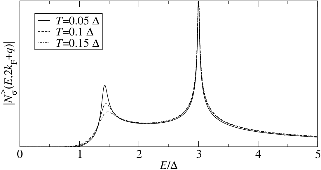
Figure 10: |Nσ>​(E,2​kF+q)||N^{>}_{\sigma}(E,2k_{\mathrm{F}}+q)| (arbitrary units) for vs​q/Δ=2v_{\mathrm{s}}q/\Delta=2, Kc=Ks=1K_{\mathrm{c}}=K_{\mathrm{s}}=1, and vc=2​vsv_{\mathrm{c}}=2v_{\mathrm{s}}. We observe spectral weight within the spin gap and a broadening of the propagating peaks, which is much stronger for the spin peak at Es=(vs​q2)2+Δ2E_{\mathrm{s}}=\sqrt{\left(\frac{v_{\mathrm{s}}q}{2}\right)^{2}+\Delta^{2}}.
Refer to caption
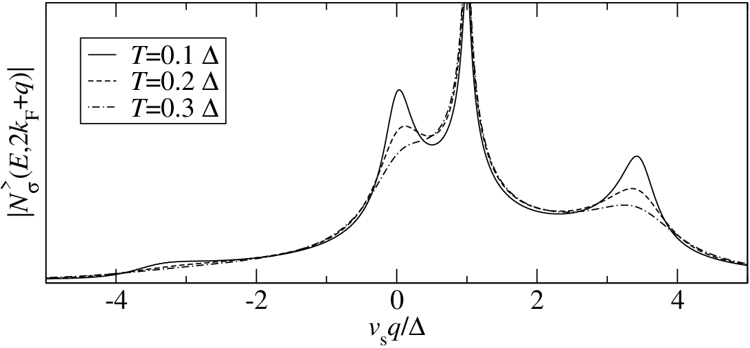
Figure 11: Constant energy scan of |Nσ>​(E,2​kF+q)||N^{>}_{\sigma}(E,2k_{\mathrm{F}}+q)| (arbitrary units) for E=2​ΔE=2\Delta, Kc=Ks=1K_{\mathrm{c}}=K_{\mathrm{s}}=1, and vc=2​vsv_{\mathrm{c}}=2v_{\mathrm{s}}. We observe a suppression of the peak at q=0q=0 related to the pinned CDW.
Refer to caption
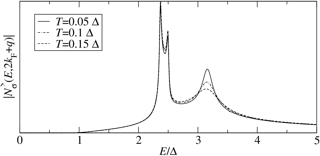
Figure 12: |Nσ>​(E,2​kF+q)||N^{>}_{\sigma}(E,2k_{\mathrm{F}}+q)| (arbitrary units) for vs​q/Δ=6v_{\mathrm{s}}q/\Delta=6, Kc=Ks=1K_{\mathrm{c}}=K_{\mathrm{s}}=1, and vs=2​vcv_{\mathrm{s}}=2v_{\mathrm{c}}. We observe again that the broadening of the propagating spin peak is stronger than that of the other peaks.

The particle contribution to the Fourier transform of the LDOS is still given by (24). The form-factor expansion in the spin sector results in the series expansion Nσ>​(E,2​kF+q)=∑iNi>​(E,2​kF+q)N^{>}_{\sigma}(E,2k_{\mathrm{F}}+q)=\sum_{i}N^{>}_{i}(E,2k_{\mathrm{F}}+q), where the first two terms can be cast in the form

Ni>​(E,2​kF+q)\displaystyle N^{>}_{i}(E,2k_{\mathrm{F}}+q) =\displaystyle= Z1​πa+b32​π5​vc​ei​π4​e−i​π2​(a+b+2​c)(vc​β)a+b−2\displaystyle\frac{Z_{1}\,\pi^{a+b}}{32\pi^{5}v_{\mathrm{c}}}\,\frac{e^{\text{i}\frac{\pi}{4}}\,e^{-\text{i}\frac{\pi}{2}(a+b+2c)}}{(v_{\mathrm{c}}\beta)^{a+b-2}} (48)
×∫−∞∞d​θ​hi​(θ)​∫−∞∞d​x​∫−∞xd​y​ei​β2​π​(Ei+vc​qi2)​xsinha⁡(x−i​δ)​ei​β2​π​(Ei−vc​qi2)​ysinhb⁡(y−i​δ)​(sinh⁡(12​(y−x))sinh⁡(12​(x+y−i​δ)))2​c,\displaystyle\times\int_{-\infty}^{\infty}d\theta\,h_{i}(\theta)\int_{-\infty}^{\infty}dx\int_{-\infty}^{x}dy\,\frac{e^{\frac{\text{i}\beta}{2\pi}(E_{i}+\frac{v_{\mathrm{c}}q_{i}}{2})x}}{\sinh^{a}(x-\text{i}\delta)}\,\frac{e^{\frac{\text{i}\beta}{2\pi}(E_{i}-\frac{v_{\mathrm{c}}q_{i}}{2})y}}{\sinh^{b}(y-\text{i}\delta)}\,\left(\frac{\sinh\bigl(\frac{1}{2}(y-x)\bigr)}{\sinh\bigl(\frac{1}{2}(x+y-\text{i}\delta)\bigr)}\right)^{2c},
h1​(θ)=1,h2​(θ)=Kσ​σ¯​(θ+i​π2)​eθ/2,E1=E2=E−Δ​cosh⁡θ,q1=q,q2=q−2​Δvs​sinh⁡θ.\displaystyle\hskip-56.9055pth_{1}(\theta)=1,\quad h_{2}(\theta)=K^{\sigma\bar{\sigma}}\bigl(\theta+\text{i}\tfrac{\pi}{2}\bigr)\,e^{\theta/2},\quad E_{1}=E_{2}=E-\Delta\cosh\theta,\quad q_{1}=q,\quad q_{2}=q-\frac{2\Delta}{v_{\mathrm{s}}}\sinh\theta.

We have plotted Nσ>​(E,2​kF+q)N^{>}_{\sigma}(E,2k_{\mathrm{F}}+q) for different temperatures in Figs. 10–12. As expected a finite temperature leads to a softening of the spectral gap Δ\Delta, a suppression of the peak related to the pinned CDW, and a broadening of the dispersing peaks. We observe that the effect of an increasing temperature on the spin peak is much stronger than the effect on the charge peak. The physical reason for this is as follows: In the CDW state only the spin sector is protected by the gap. Thus for T≪ΔT\ll\Delta there exists a significant number of antiholons in the thermal ground state. They will participate in the distribution of the external momentum qq after the creation of an additional antiholon-spinon pair, thus leading to a decreased probability for the spinon to take the momentum qq and thus to a suppression of the spin peak following Es​(q)E_{\mathrm{s}}(q). On the other hand, the charge peak is not affected as the antiholons possess a linear dispersion. This behavior is reminiscent of what is found for the bulk spectral functions [51].

VII Implications for STM experiments

STM experiments measure the local tunneling current, which is related to the LDOS by Eq. (1). In particular, the voltage dependence of the tunneling conductance measures the thermally smeared LDOS of the sample at the position of the tip. A possible spin dependence in the LDOS can be detected using a magnetic tip. As we have considered a one-dimensional model, our results apply to quasi-1D materials at energies above the 1D-3D cross-over scale, which is set by the strength of the 3D couplings. Furthermore, the main feature of the model we have studied is the existence of a spectral gap in one of the sectors, while the excitations in the other sector remain gapless. This situation is experimentally realized in various materials, for example in two-leg ladder materials [17], stripe phases of HTSC [5, 9], carbon nanotubes [1, 16], Bechgaard salts [14], and chain materials [15] like SrCuO2{\rm SrCuO_{2}} and Sr2​CuO3{\rm Sr_{2}CuO_{3}}. As our results show, STM experiments can be used to extract rather detailed information regarding bulk excitations by analyzing the modification of the LDOS due to a boundary/impurity.

Perhaps the most interesting materials to which our findings may be applied on a qualitative level are two-leg ladders like [59] Sr14Cu24O41 which possesses a spin gap [60] of Δ≈550​K\Delta\approx 550K. The model we have studied captures the most basic features of the low-energy description of (weakly doped) two-leg ladders, namely a gapless charge sector and a gapped spin sector. While the description of the spin sector for weakly doped two-leg ladders is considerably more involved, we expect the gross features to be similar. In particular, we expect peaks to appear in Nσ​(E,Q)N_{\sigma}(E,Q), which correspond to the pinned CDW order, dispersing spin and charge degrees of freedom, and possibly boundary bound states. We note that our results apply to the regime T≪E,Δ,vc/a0T\ll E,\Delta,v_{\mathrm{c}}/a_{0}, where temperature effects are negligible.

In Ref. [9] it was proposed that STM and STS experiments in HTSC can be used to detect “fluctuating stripes” (i.e. incommensurate spin and charge fluctuations on energy scales small compared to the superconducting gap) by rendering them static by the effects of impurities with a potential comparable to the (low) energy scales of these fluctuations. In that work it was also argued that 1D Luttinger liquids are effectively quantum critical systems and that a form of local (power law) CDW order is effectively induced by impurities (and edges) which pin the phase of the CDW, an effect that we have shown here to take place in a 1D Luther-Emery liquid associated with a CDW. STM and STS experiments in Bi2Sr2CaCu2O8+δ have confirmed the existence of both non-dispersive spectral features in the LDOS associated with “fluctuating stripe order” as well as dispersive features associated with the propagating quasiparticles of the superconductor[2, 9, 4]. Recent STS experiments in Bi2Sr2CaCu2O8+δ have shown that the dispersive features of the LDOS disappear above the TcT_{\mathrm{c}} of the superconductor while the non-dispersive features survive up to the temperature T∗T^{*} at which the pseudogap closes[61].

VIII Conclusions

In this work we have determined the spatial Fourier transform of the LDOS of one-dimensional CDW states and Mott insulators in presence of a boundary. The latter may either model a strong potential impurity or be realized in a two-tip STM experiment. We found that the Fourier transform of the LDOS is dominated by a singularity at an energy equal to the single-particle gap Δ\Delta and at momentum 2​kF2k_{\mathrm{F}}. This feature is indicative of the pinning of the CDW order at the position of the impurity. We observed clear signatures of dispersing spin and charge excitations, which can be used to infer the nature of the underlying electron-electron interactions. In the case of CDW states with repulsive interactions we find a spin mode and a linear dispersing charge mode while for attractive interactions a third dispersing mode appears, which can be thought of as arising from a spin excitation with a fixed momentum q0q_{0} and a charge excitation with momentum q−q0q-q_{0}.

We have also investigated the modification of the LDOS due to boundary bound states. These may arise in presence of boundary potentials or magnetic fields. We found that boundary bound states give rise to non-dispersing singularities at energies below the single-particle gap. While the bound state is formed in the gapped sector of the theory, the exponent of the corresponding singularity only depends on the Luttinger liquid parameter of the gapless sector. We have analyzed temperature effects in regime T≪ΔT\ll\Delta and discussed implications of our results for STM measurements on quasi-1D materials such as doped two-leg ladders.

Acknowledgments

We would like to thank Joe Bhaseen, Dmitry Kovrizhin, and Christian Pfleiderer for useful discussions. DS was supported by the Deutsche Akademie der Naturforscher Leopoldina under grant BMBF-LPD 9901/8-145 while working at the Rudolf Peierls Centre for Theoretical Physics, University of Oxford. This work was also supported by the EPSRC under grant EP/D050952/1 (FHLE), the NSF under grant DMR 0758462 at the University of Illinois (EF), the U.S. Department of Energy, Division of Materials Sciences under Award No. DE-FG02-07ER46453 through the Frederick Seitz Materials Research Laboratory of the University of Illinois (EF, AJ) and the ESF network INSTANS.

Appendix A Renormalization group analysis of an impurity potential

Let us consider the low-energy theory of a one-dimensional CDW state on the infinite line H=Hc+HsH=H_{\mathrm{c}}+H_{\mathrm{s}}, where

Hc\displaystyle H_{\mathrm{c}} =\displaystyle= vc16​π∫−∞∞dx[1Kc2(∂xΦc)2+Kc2(∂xΘc)2],\displaystyle\frac{v_{\mathrm{c}}}{16\pi}\int_{-\infty}^{\infty}dx\biggl[\frac{1}{K_{\mathrm{c}}^{2}}\bigr(\partial_{x}\Phi_{\mathrm{c}}\bigr)^{2}+K_{\mathrm{c}}^{2}\bigr(\partial_{x}\Theta_{\mathrm{c}}\bigr)^{2}\biggr], (49)
Hs\displaystyle H_{\mathrm{s}} =\displaystyle= vs16​π∫−∞∞dx[1Ks2(∂xΦs)2+Ks2(∂xΘs)2]−gs(2​π)2∫−∞∞dxcosΦs.\displaystyle\frac{v_{\mathrm{s}}}{16\pi}\int_{-\infty}^{\infty}dx\biggl[\frac{1}{K_{\mathrm{s}}^{2}}\bigr(\partial_{x}\Phi_{\mathrm{s}}\bigr)^{2}+K_{\mathrm{s}}^{2}\bigr(\partial_{x}\Theta_{\mathrm{s}}\bigr)^{2}\biggr]-\frac{g_{\mathrm{s}}}{(2\pi)^{2}}\int_{-\infty}^{\infty}dx\,\cos\Phi_{\mathrm{s}}. (50)

We want to study the effect of an impurity potential at position x=0x=0, which in bosonized form reads

Vimp=λ​∫−∞∞d​x​δ​(x)​cos⁡(Φc2)​cos⁡(Φs2).V_{\mathrm{imp}}=\lambda\int_{-\infty}^{\infty}dx\,\delta(x)\,\cos\left(\frac{\Phi_{\mathrm{c}}}{2}\right)\cos\left(\frac{\Phi_{\mathrm{s}}}{2}\right). (51)

As the spin sector in the bulk is massive, we have ⟨cos⁡(Φs/2)⟩≠0\big\langle\!\cos(\Phi_{\mathrm{s}}/2)\big\rangle\neq 0, which implies that at low energies we can approximate cos⁡(Φc/2)​cos⁡(Φs/2)\cos\bigl(\Phi_{\mathrm{c}}/2\bigr)\cos\bigl(\Phi_{\mathrm{s}}/2\bigr) in (51) by ⟨cos⁡(Φc/2)⟩​cos⁡(Φs/2)+cos⁡(Φc/2)​⟨cos⁡(Φs/2)⟩\big\langle\!\cos\bigl(\Phi_{\mathrm{c}}/2\bigr)\big\rangle\cos\bigl(\Phi_{\mathrm{s}}/2\bigr)+\cos\bigl(\Phi_{\mathrm{c}}/2\bigr)\big\langle\!\cos\bigl(\Phi_{\mathrm{s}}/2\bigr)\big\rangle. Thus in the charge sector we get a boundary sine-Gordon model [62]. For Kc2<2K_{\mathrm{c}}^{2}<2 the impurity scattering potential scales to strong coupling. Hence as long as the interactions are not too attractive the field Φc\Phi_{\mathrm{c}} gets pinned at the boundary, Φc​(0)=0\Phi_{\mathrm{c}}(0)=0. This in turn induces an impurity contribution in the gapped spin sector

Vimp,s=λ⁡⟨cos⁡(Φc​(0)2)⟩​∫−∞∞d​x​δ​(x)​cos⁡(Φs2).V_{\mathrm{imp,s}}=\lambda\,\left\langle\cos\left(\frac{\Phi_{\mathrm{c}}(0)}{2}\right)\right\rangle\;\int_{-\infty}^{\infty}dx\,\delta(x)\,\cos\left(\frac{\Phi_{\mathrm{s}}}{2}\right). (52)

If one analyzes the bulk and boundary cosine terms in the resulting impurity model (50) and (52) simultaneously, the leading order renormalization group equations are given by the scaling dimensions of the perturbing operators

d​gsd​l=2​(1−Ks2)​gs,d​λd​l=(1−Ks22)​λ.\frac{dg_{\mathrm{s}}}{dl}=2\,\bigl(1-K_{\mathrm{s}}^{2}\bigr)\,g_{\mathrm{s}},\quad\frac{d\lambda}{dl}=\left(1-\frac{K_{\mathrm{s}}^{2}}{2}\right)\lambda. (53)

As long as Ks2>2/3K_{\mathrm{s}}^{2}>2/3 the boundary term grows more rapidly than the bulk term. Assuming that it reaches the strong-coupling regime first leads to the pinning of the spin field Φs​(0)=0\Phi_{\mathrm{s}}(0)=0. This cuts the chain in two half-lines and we obtain the model (12)–(15).

Appendix B Calculation of the Green function: Charge sector

The Green function (16) factorizes into a product of correlation functions in the spin and charge sectors. For example, using the bosonization identities (7) and (8) the 2​kF2k_{\mathrm{F}}-component Gσ​σ′R​LG^{RL}_{\sigma\sigma^{\prime}} can be written as

Gσ​σ′R​L​(τ,x1,x2)=−12​π​⟨e−i2​ϕc​(τ,x1)​e−i2​ϕ¯c​(0,x2)⟩c​⟨e−i2​fσ​ϕs​(τ,x1)​e−i2​fσ′​ϕ¯s​(0,x2)⟩s.G^{RL}_{\sigma\sigma^{\prime}}(\tau,x_{1},x_{2})=-\frac{1}{2\pi}\,\Big\langle e^{-\frac{\text{i}}{2}\phi_{\mathrm{c}}(\tau,x_{1})}\,e^{-\frac{\text{i}}{2}\bar{\phi}_{\mathrm{c}}(0,x_{2})}\Big\rangle_{\mathrm{c}}\,\Big\langle e^{-\frac{\text{i}}{2}f_{\sigma}\phi_{\mathrm{s}}(\tau,x_{1})}\,e^{-\frac{\text{i}}{2}f_{\sigma^{\prime}}\bar{\phi}_{\mathrm{s}}(0,x_{2})}\Big\rangle_{\mathrm{s}}. (54)

Both correlation functions have to be determined in the presence of the boundary at x=0x=0. The charge part is calculated below using a standard mode expansion [36], the spin part will be calculated in App. C.

In order to obtain the correlation functions in the charge sector we first bring the Hamiltonian (13) to standard form by rescaling the fields as Φc→Kc​Φc\Phi_{\mathrm{c}}\rightarrow K_{\mathrm{c}}\Phi_{\mathrm{c}}, Θc→Θc/Kc\Theta_{\mathrm{c}}\rightarrow\Theta_{\mathrm{c}}/K_{\mathrm{c}}. The charge parts of the operators (7) and (8) then become

exp⁡(±i2​ϕc​(τ,x))\displaystyle\exp\Bigl(\pm\tfrac{\text{i}}{2}\phi_{\mathrm{c}}(\tau,x)\Bigr) →\displaystyle\rightarrow ei​π​s​c/4exp(±i2cϕc(z))exp(±i2sϕ¯c(z¯))=e−iπsc/4exp(±i2sϕ¯c(z¯))exp(±i2cϕc(z)),\displaystyle e^{\text{i}\pi sc/4}\exp\Bigl(\pm\tfrac{\text{i}}{2}c\,\phi_{\mathrm{c}}(z)\Bigr)\exp\Bigl(\pm\tfrac{\text{i}}{2}s\,\bar{\phi}_{\mathrm{c}}(\bar{z})\Bigr)=e^{-\text{i}\pi sc/4}\exp\Bigl(\pm\tfrac{\text{i}}{2}s\,\bar{\phi}_{\mathrm{c}}(\bar{z})\Bigr)\exp\Bigl(\pm\tfrac{\text{i}}{2}c\,\phi_{\mathrm{c}}(z)\Bigr), (55)
exp⁡(±i2​ϕ¯c​(τ,x))\displaystyle\exp\Bigl(\pm\tfrac{\text{i}}{2}\bar{\phi}_{\mathrm{c}}(\tau,x)\Bigr) →\displaystyle\rightarrow ei​π​s​c/4exp(±i2sϕc(z))exp(±i2cϕ¯c(z¯))=e−iπsc/4exp(±i2cϕ¯c(z¯))exp(±i2sϕc(z)),\displaystyle e^{\text{i}\pi sc/4}\exp\Bigl(\pm\tfrac{\text{i}}{2}s\,\phi_{\mathrm{c}}(z)\Bigr)\exp\Bigl(\pm\tfrac{\text{i}}{2}c\,\bar{\phi}_{\mathrm{c}}(\bar{z})\Bigr)=e^{-\text{i}\pi sc/4}\exp\Bigl(\pm\tfrac{\text{i}}{2}c\,\bar{\phi}_{\mathrm{c}}(\bar{z})\Bigr)\exp\Bigl(\pm\tfrac{\text{i}}{2}s\,\phi_{\mathrm{c}}(z)\Bigr), (56)

where we have already used (60) and assumed −L<x<0-L<x<0. The constants are parameterized via s=sinh⁡ξcs=\sinh\xi_{\mathrm{c}} and c=cosh⁡ξcc=\cosh\xi_{\mathrm{c}} with Kc=eξcK_{\mathrm{c}}=e^{\xi_{\mathrm{c}}}. The complex coordinates are defined as z=vc​τ−i​xz=v_{\mathrm{c}}\tau-\text{i}x, z¯=vc​τ+i​x\bar{z}=v_{\mathrm{c}}\tau+\text{i}x. The charge part of the Green function can hence be obtained from the four-point function

⟨ei​β1​ϕ¯c​(z¯1)​ei​α1​ϕc​(z1)​ei​α2​ϕc​(z2)​ei​β2​ϕ¯c​(z¯2)⟩UHP,\Big\langle e^{\text{i}\beta_{1}\bar{\phi}_{\mathrm{c}}(\bar{z}_{1})}\,e^{\text{i}\alpha_{1}\phi_{\mathrm{c}}(z_{1})}\,e^{\text{i}\alpha_{2}\phi_{\mathrm{c}}(z_{2})}\,e^{\text{i}\beta_{2}\bar{\phi}_{\mathrm{c}}(\bar{z}_{2})}\Big\rangle_{\mathrm{UHP}}, (57)

where α1,2,β1,2∈ℝ\alpha_{1,2},\beta_{1,2}\in\mathbb{R}, z1=vc​τ−i​x1z_{1}=v_{\mathrm{c}}\tau-\text{i}x_{1} and z2=−i​x2z_{2}=-\text{i}x_{2} lie in the upper half-plane.

We calculate (57) from the mode expansions for the chiral fields ϕc\phi_{\mathrm{c}} and ϕ¯c\bar{\phi}_{\mathrm{c}}. These are obtained by first noting that the fields Φc\Phi_{\mathrm{c}} and Θc\Theta_{\mathrm{c}} have to satisfy the equations of motion vc∂xΘc=−i∂τΦcv_{\mathrm{c}}\partial_{x}\Theta_{\mathrm{c}}=-\text{i}\partial_{\tau}\Phi_{\mathrm{c}} and ∂τΘc=i​vc​∂xΦc\partial_{\tau}\Theta_{\mathrm{c}}=\text{i}v_{\mathrm{c}}\partial_{x}\Phi_{\mathrm{c}} as well as the boundary conditions Φc​(x=0)=Φc​(x=−L)=0\Phi_{\mathrm{c}}(x=0)=\Phi_{\mathrm{c}}(x=-L)=0. The semi-infinite system is obtained by taking L→∞L\rightarrow\infty. This yields the mode expansions

Φc​(τ,x)\displaystyle\Phi_{\mathrm{c}}(\tau,x) =\displaystyle= −xLΠ^0+i∑n=1∞sin⁡n​π​xLn​π(bne−nπvcτ/L−bn†en​π​vc​τ/L),\displaystyle-\frac{x}{L}\hat{\Pi}_{0}+\text{i}\sum_{n=1}^{\infty}\frac{\sin\frac{n\pi x}{L}}{\sqrt{n\pi}}\left(b_{n}\,e^{-n\pi v_{\mathrm{c}}\tau/L}-b_{n}^{\dagger}\,e^{n\pi v_{\mathrm{c}}\tau/L}\right), (58)
Θc​(τ,x)\displaystyle\Theta_{\mathrm{c}}(\tau,x) =\displaystyle= Θ^0−ivc​τLΠ^0+∑n=1∞cos⁡n​π​xLn​π(bne−nπvcτ/L+bn†en​π​vc​τ/L),\displaystyle\hat{\Theta}_{0}-\text{i}\,\frac{v_{\mathrm{c}}\tau}{L}\hat{\Pi}_{0}+\sum_{n=1}^{\infty}\frac{\cos\frac{n\pi x}{L}}{\sqrt{n\pi}}\left(b_{n}\,e^{-n\pi v_{\mathrm{c}}\tau/L}+b_{n}^{\dagger}\,e^{n\pi v_{\mathrm{c}}\tau/L}\right), (59)

where the zero-mode operator Π^0\hat{\Pi}_{0} has the discrete spectrum 2​π​m2\pi m, m∈ℤm\in\mathbb{Z}, and [Θ^0,Π^0]=8​π​i\left[\hat{\Theta}_{0},\hat{\Pi}_{0}\right]=8\pi\text{i}, [bm,bn†]=8​π​δm​n\left[b_{m},b_{n}^{\dagger}\right]=8\pi\,\delta_{mn}. The mode expansions for the chiral fields are easily obtained via ϕc=(Φc+Θc)/2\phi_{\mathrm{c}}=(\Phi_{\mathrm{c}}+\Theta_{\mathrm{c}})/2 and ϕ¯c=(Φc−Θc)/2\bar{\phi}_{\mathrm{c}}=(\Phi_{\mathrm{c}}-\Theta_{\mathrm{c}})/2. Their commutation relations are

[ϕc​(τ,x),ϕ¯c​(τ,x′)]={0,x=x′=0,4​π​i,x=x′=−L,2​π​i,else,\bigl[\phi_{\mathrm{c}}(\tau,x),\bar{\phi}_{\mathrm{c}}(\tau,x^{\prime})\bigr]=\left\{\begin{array}[]{lll}0&,&x=x^{\prime}=0,\\ 4\pi\text{i}&,&x=x^{\prime}=-L,\\ 2\pi\text{i}&,&\text{else},\end{array}\right. (60)

as well as [ϕc​(τ,x),ϕc​(τ,x′)]=−[ϕ¯c​(τ,x),ϕ¯c​(τ,x′)]=2​π​i​sgn​(x−x′)\bigl[\phi_{\mathrm{c}}(\tau,x),\phi_{\mathrm{c}}(\tau,x^{\prime})\bigr]=-\bigl[\bar{\phi}_{\mathrm{c}}(\tau,x),\bar{\phi}_{\mathrm{c}}(\tau,x^{\prime})\bigr]=2\pi\text{i}\,\text{sgn}(x-x^{\prime})\,, where sgn​(0)=0\text{sgn}(0)\,=0. Similar mode expansions were obtained in Refs. [36]. Given the mode expansion it is straightforward to calculate the four-point function (57). We find

⟨ei​β1​ϕ¯c​(z¯1)​ei​α1​ϕc​(z1)​ei​α2​ϕc​(z2)​ei​β2​ϕ¯c​(z¯2)⟩UHP=C​δα1+α2,β1+β2​(z1−z2)2​α1​α2​(z¯1−z¯2)2​β1​β2(z¯1−z1)2​α1​β1​(z¯1−z2)2​α2​β1​(z1−z¯2)2​α1​β2​(z2−z¯2)2​α2​β2,\Big\langle e^{\text{i}\beta_{1}\bar{\phi}_{\mathrm{c}}(\bar{z}_{1})}\,e^{\text{i}\alpha_{1}\phi_{\mathrm{c}}(z_{1})}\,e^{\text{i}\alpha_{2}\phi_{\mathrm{c}}(z_{2})}\,e^{\text{i}\beta_{2}\bar{\phi}_{\mathrm{c}}(\bar{z}_{2})}\Big\rangle_{\mathrm{UHP}}=\frac{C\delta_{\alpha_{1}+\alpha_{2},\beta_{1}+\beta_{2}}\ (z_{1}-z_{2})^{2\alpha_{1}\alpha_{2}}\,(\bar{z}_{1}-\bar{z}_{2})^{2\beta_{1}\beta_{2}}}{(\bar{z}_{1}-z_{1})^{2\alpha_{1}\beta_{1}}(\bar{z}_{1}-z_{2})^{2\alpha_{2}\beta_{1}}(z_{1}-\bar{z}_{2})^{2\alpha_{1}\beta_{2}}(z_{2}-\bar{z}_{2})^{2\alpha_{2}\beta_{2}}}\ , (61)

where C∈ℝC\in\mathbb{R} is a constant which we set to one throughout this manuscript. This result implies Eq. (19). The finite-temperature correlation functions are obtained [58, 38] by mapping (61) onto a cylinder of circumference vc/kB​Tv_{\mathrm{c}}/k_{\mathrm{B}}T.

Appendix C Calculation of the Green function: Spin sector

The calculation of the correlation functions in the spin sector relies on the integrability of the sine-Gordon model on the half-line. We use the boundary state formalism introduced by Ghoshal and Zamolodchikov [29] together with a form-factor expansion based on form factors obtained by Lukyanov and Zamolodchikov [42]. The analogous expansion for the quantum Ising model has been analyzed in Ref. [48]. We will first discuss the general formalism and then derive (20).

C.1 Boundary state formalism and form-factor expansion

Refer to caption
Refer to caption
Figure 13: Two-particle scattering and scattering off the boundary.

Let us consider the sine-Gordon model (14) in the half-plane (τ,x)(\tau,x), τ∈ℝ\tau\in\mathbb{R}, −∞<x≤0-\infty<x\leq 0. The boundary is located at x=0x=0 and τ\tau denotes imaginary time (τ=i​t\tau=\text{i}t). The Hilbert space of states associated with the semi-infinite line τ=const\tau=\text{const}, −∞<x≤0-\infty<x\leq 0, is denoted by ℋb\mathcal{H}_{\mathrm{b}}. We obtain the Euclidean action in its standard form by rescaling the fields according to Φs→Φs′=Φs/Ks\Phi_{\mathrm{s}}\rightarrow\Phi_{\mathrm{s}}^{\prime}=\Phi_{\mathrm{s}}/K_{\mathrm{s}} and Θs→Θs′=Ks​Θs\Theta_{\mathrm{s}}\rightarrow\Theta_{\mathrm{s}}^{\prime}=K_{\mathrm{s}}\Theta_{\mathrm{s}}. The action of the sine-Gordon model with a boundary is then given by [29] (we set vs=1v_{\mathrm{s}}=1)

𝒮bsG=116​π​∫d​τ​∫−∞0d​x​[(∂τΦs′)2+(∂xΦs′)2−4​gsπ​cos⁡(Ks​Φs′)]−gb​∫d​τ​cos⁡(Ks2​(Φs′|x=0−Φs0/Ks)),\mathcal{S}_{\mathrm{bsG}}=\frac{1}{16\pi}\int d\tau\int_{-\infty}^{0}dx\biggl[\bigl(\partial_{\tau}\Phi_{\mathrm{s}}^{\prime}\bigr)^{2}+\bigl(\partial_{x}\Phi_{\mathrm{s}}^{\prime}\bigr)^{2}-\frac{4g_{\mathrm{s}}}{\pi}\cos\bigl(K_{\mathrm{s}}\Phi_{\mathrm{s}}^{\prime}\bigr)\biggr]-g_{\mathrm{b}}\int d\tau\,\cos\left(\frac{K_{\mathrm{s}}}{2}\bigl(\Phi_{\mathrm{s}}^{\prime}\big|_{x=0}-\Phi_{\mathrm{s}}^{0}/K_{\mathrm{s}}\bigr)\right), (62)

where gsg_{\mathrm{s}}, gbg_{\mathrm{b}} and Φs0\Phi_{\mathrm{s}}^{0} are free parameters. (We use the conventions 0<Ks<10<K_{\mathrm{s}}<1, the action as given in Ref. [29] is obtained by another rescaling of the fields by 8​π\sqrt{8\pi}.) The cases gb=0g_{\mathrm{b}}=0 and gb→∞g_{\mathrm{b}}\rightarrow\infty correspond to free and fixed boundary conditions, respectively. We stress that in the case of fixed boundary conditions Φs′​(x=0)=Φs0/Ks\Phi_{\mathrm{s}}^{\prime}(x=0)=\Phi_{\mathrm{s}}^{0}/K_{\mathrm{s}} implies Φs​(x=0)=Φs0\Phi_{\mathrm{s}}(x=0)=\Phi_{\mathrm{s}}^{0} in the original system (14). As was conjectured by Ghoshal and Zamolodchikov [29] and shown independently [30] by MacIntyre and Saleur, Skorik and Warner, the classical sine-Gordon model on the half-line (62) possesses infinitely many integrals of motion and is hence integrable.

We start by summarizing some results for the bulk sine-Gordon model, i.e. the theory without boundary. In the repulsive regime (Ks>1/2K_{\mathrm{s}}>1/\sqrt{2}) a basis of the Hilbert space ℋ\mathcal{H} is given by scattering states of solitons and antisolitons

|θ1,…,θn⟩a1,…,an=Za1†(θ1)…Zan†(θn)|0⟩,an,…,a1⟨θn,…,θ1|=⟨0|Zan(θn)…Za1(θ1),\left|\theta_{1},\ldots,\theta_{n}\right\rangle_{a_{1},\ldots,a_{n}}=Z^{\dagger}_{a_{1}}(\theta_{1})\ldots Z^{\dagger}_{a_{n}}(\theta_{n})\left|0\right\rangle,\quad^{a_{n},\ldots,a_{1}}\!\!\left\langle\theta_{n},\ldots,\theta_{1}\right|=\left\langle 0\right|Z_{a_{n}}(\theta_{n})\ldots Z_{a_{1}}(\theta_{1}), (63)

where ai=±1a_{i}=\pm 1 and |0⟩\left|0\right\rangle is the ground state in absence of a boundary. Solitons and antisolitons are created by the operators Z−†​(θ)Z^{\dagger}_{-}(\theta) and Z+†​(θ)Z^{\dagger}_{+}(\theta). They are characterized by a topological U(1) charge −1-1 and 11, respectively, while their energy and momentum are parametrized in terms of the rapidity θ\theta by E=Δ​cosh⁡θE=\Delta\cosh\theta and P=Δ​sinh⁡θP=\Delta\sinh\theta. The dependence of the soliton mass Δ\Delta on the bare parameters in the action was obtained in Ref. [64]. We note that in the attractive regime (Ks<1/2K_{\mathrm{s}}<1/\sqrt{2}) breather (soliton-antisoliton) bound states occur as well. The operators ZaZ_{a} and Za†Z_{a}^{\dagger} fulfill the Faddeev–Zamolodchikov algebra [65] (see Fig. 13)

Za1​(θ1)​Za2​(θ2)\displaystyle Z_{a_{1}}(\theta_{1})Z_{a_{2}}(\theta_{2}) =\displaystyle= Sa1​a2b1​b2​(θ1−θ2)​Zb2​(θ2)​Zb1​(θ1),\displaystyle S_{a_{1}a_{2}}^{b_{1}b_{2}}(\theta_{1}-\theta_{2})Z_{b_{2}}(\theta_{2})Z_{b_{1}}(\theta_{1}),
Za1†​(θ1)​Za2†​(θ2)\displaystyle Z_{a_{1}}^{\dagger}(\theta_{1})Z_{a_{2}}^{\dagger}(\theta_{2}) =\displaystyle= Sa1​a2b1​b2​(θ1−θ2)​Zb2†​(θ2)​Zb1†​(θ1),\displaystyle S_{a_{1}a_{2}}^{b_{1}b_{2}}(\theta_{1}-\theta_{2})Z_{b_{2}}^{\dagger}(\theta_{2})Z_{b_{1}}^{\dagger}(\theta_{1}), (64)
Za1​(θ1)​Za2†​(θ2)\displaystyle Z_{a_{1}}(\theta_{1})Z_{a_{2}}^{\dagger}(\theta_{2}) =\displaystyle= 2​π​δ​(θ1−θ2)​δa1​a2+Sa2​b1b2​a1​(θ1−θ2)​Zb2†​(θ2)​Zb1​(θ1).\displaystyle 2\pi\delta(\theta_{1}-\theta_{2})\delta_{a_{1}a_{2}}+S_{a_{2}b_{1}}^{b_{2}a_{1}}(\theta_{1}-\theta_{2})Z_{b_{2}}^{\dagger}(\theta_{2})Z_{b_{1}}(\theta_{1}).

Here Sa1​a2b1​b2​(θ)S_{a_{1}a_{2}}^{b_{1}b_{2}}(\theta) is the two-particle scattering matrix, which was derived in Refs. [32, 66]. The unitarity condition reads Sa1​a2c1​c2​(θ)​Sc1​c2b1​b2​(−θ)=δa1b1​δa2b2S_{a_{1}a_{2}}^{c_{1}c_{2}}(\theta)S_{c_{1}c_{2}}^{b_{1}b_{2}}(-\theta)=\delta_{a_{1}}^{b_{1}}\delta_{a_{2}}^{b_{2}}. Its non-vanishing elements are

S+⁣++⁣+​(θ)=S−⁣−−⁣−​(θ),S+⁣−+⁣−​(θ)=S−⁣+−⁣+​(θ),S−⁣++⁣−​(θ)=S+⁣−−⁣+​(θ),S^{++}_{++}(\theta)=S^{--}_{--}(\theta),\quad S^{+-}_{+-}(\theta)=S^{-+}_{-+}(\theta),\quad S^{+-}_{-+}(\theta)=S^{-+}_{+-}(\theta), (65)

for which explicit expressions can be found for example in Ref. [44]. At the LEP (Ks=1/2K_{\mathrm{s}}=1/\sqrt{2}) the scattering matrix simplifies to Sa1​a2b1​b2​(θ)=−δa1b1​δa2b2S_{a_{1}a_{2}}^{b_{1}b_{2}}(\theta)=-\delta_{a_{1}}^{b_{1}}\delta_{a_{2}}^{b_{2}}, while in the spin symmetric case (Ks=1K_{\mathrm{s}}=1) one has [46]

S+⁣++⁣+​(θ)=S0​(θ)≡−Γ⁡(1+i​θ2​π)​Γ​(12−i​θ2​π)Γ⁡(1−i​θ2​π)​Γ​(12+i​θ2​π),S+⁣−+⁣−​(θ)=−θθ−i​π​S0​(θ),S−⁣++⁣−​(θ)=−i​πθ−i​π​S0​(θ).S^{++}_{++}(\theta)=S_{0}(\theta)\equiv-\frac{\Gamma\bigl(1+\tfrac{\text{i}\theta}{2\pi}\bigr)\,\Gamma\bigl(\tfrac{1}{2}-\tfrac{\text{i}\theta}{2\pi}\bigr)}{\Gamma\bigl(1-\tfrac{\text{i}\theta}{2\pi}\bigr)\,\Gamma\bigl(\tfrac{1}{2}+\tfrac{\text{i}\theta}{2\pi}\bigr)},\quad S^{+-}_{+-}(\theta)=-\frac{\theta}{\theta-\text{i}\pi}\,S_{0}(\theta),\quad S^{+-}_{-+}(\theta)=-\frac{\text{i}\pi}{\theta-\text{i}\pi}\,S_{0}(\theta). (66)

We note that the Faddeev–Zamolodchikov algebra (64) is invariant under the unitary transformation Za​(θ)→ei​φ​Za​(θ)Z_{a}(\theta)\rightarrow e^{\text{i}\varphi}Z_{a}(\theta), which changes the basis of scattering states. In terms of the basis states (63) the resolution of the identity reads

id=|0⟩⟨0|+∑n=1∞1n!∑{ai}∫−∞∞d​θ1​…​d​θn(2​π)n|θn,…,θ1⟩an,…,a1a1,…,an⟨θ1,…,θn|.\mathrm{id}=\left|0\right\rangle\left\langle 0\right|+\sum_{n=1}^{\infty}\frac{1}{n!}\sum_{\{a_{i}\}}\int_{-\infty}^{\infty}\frac{d\theta_{1}\ldots d\theta_{n}}{(2\pi)^{n}}\left|\theta_{n},\ldots,\theta_{1}\right\rangle_{a_{n},\ldots,a_{1}}\,\!\!^{a_{1},\ldots,a_{n}}\!\!\left\langle\theta_{1},\ldots,\theta_{n}\right|. (67)

The boundary can be introduced[29] as an infinitely heavy, impenetrable particle BB sitting at x=0x=0. The ground state in presence of the boundary can then be represented as |0b⟩=B|0⟩\left|0_{\mathrm{b}}\right\rangle=B\left|0\right\rangle. Scattering of elementary excitations off the boundary is encoded in the relations (see Fig. 13)

Za†​(θ)​B=Rab​(θ)​Zb†​(−θ)​B,Z_{a}^{\dagger}(\theta)B=R_{a}^{b}(\theta)Z_{b}^{\dagger}(-\theta)B, (68)

where the functions Rab​(θ)R_{a}^{b}(\theta) are the single-particle reflection amplitudes. In order to preserve integrability, the boundary reflection matrix R⁡(θ)R(\theta) has to satisfy a number of conditions which were discussed in Ref. [29]. At the LEP and for Dirichlet boundary conditions Φs​(τ,x=0)=Φs0\Phi_{\mathrm{s}}(\tau,x=0)=\Phi_{\mathrm{s}}^{0}, 0≤Φs0<π0\leq\Phi_{\mathrm{s}}^{0}<\pi in the original system (14), it is given by [45]

R±±​(θ)=−cosh⁡(i​π4±i​Φs02+θ2)cosh⁡(i​π4±i​Φs02−θ2),R±∓​(θ)=0.R_{\pm}^{\pm}(\theta)=-\frac{\cosh\Bigl(\text{i}\frac{\pi}{4}\pm\text{i}\frac{\Phi_{\mathrm{s}}^{0}}{2}+\frac{\theta}{2}\Bigr)}{\cosh\left(\text{i}\frac{\pi}{4}\pm\text{i}\frac{\Phi_{\mathrm{s}}^{0}}{2}-\frac{\theta}{2}\right)},\quad R_{\pm}^{\mp}(\theta)=0. (69)

For π/2≤Φs0\pi/2\leq\Phi_{\mathrm{s}}^{0} the reflection amplitude R++R^{+}_{+} possesses a simple pole in the physical strip 0≤ℑ​𝔪​θ≤π/20\leq\mathfrak{Im}\,\theta\leq\pi/2, which indicates the existence of a boundary bound state. The overall sign of the reflection matrix is fixed by the requirement −iRes[R±±(θ),θ=±i(Φs0∓π/2)]=−2cosΦs0>0-\text{i}\,\text{Res}\bigl[R^{\pm}_{\pm}(\theta),\theta=\pm\text{i}\,(\Phi_{\mathrm{s}}^{0}\mp\pi/2)\bigr]=-2\cos\Phi_{\mathrm{s}}^{0}>0, see App. C.5 below. Explicit representations of RR for general KsK_{\mathrm{s}} can be found in Refs. [29, 46, 47]. For Ks=1K_{\mathrm{s}}=1 and Φs0=0\Phi_{\mathrm{s}}^{0}=0 one finds in particular

R±±​(θ)=−Γ⁡(1+i​θ2​π)​Γ​(12−i​θπ)π​Γ​(1−i​θ2​π)​ 2iπ​θ​(cosh⁡θ2+i​sinh⁡θ2),R±∓​(θ)=0.R_{\pm}^{\pm}(\theta)=-\frac{\Gamma\bigl(1+\tfrac{\text{i}\theta}{2\pi}\bigr)\,\Gamma\bigl(\tfrac{1}{2}-\tfrac{\text{i}\theta}{\pi}\bigr)}{\sqrt{\pi}\,\Gamma\bigl(1-\tfrac{\text{i}\theta}{2\pi}\bigr)}\,2^{\frac{\text{i}}{\pi}\theta}\,\left(\cosh\frac{\theta}{2}+\text{i}\sinh\frac{\theta}{2}\right),\quad R_{\pm}^{\mp}(\theta)=0. (70)

The vanishing of the off-diagonal amplitudes R±∓​(θ)=0R_{\pm}^{\mp}(\theta)=0 is a consequence of fixed boundary conditions and holds for general KsK_{\mathrm{s}}.

Our aim is to calculate the time-ordered two-point function

C(τ,x1,x2)=⟨0b|𝒯τO1(τ,x1)O2(0,x2)|0b⟩.C(\tau,x_{1},x_{2})=\left\langle 0_{\mathrm{b}}\right|\mathcal{T}_{\tau}\,O_{1}(\tau,x_{1})\,O_{2}(0,x_{2})\left|0_{\mathrm{b}}\right\rangle. (71)

Here the time-dependence of the operators is given by Oi​(τ,x)=eτ​Hb​Oi​(0,x)​e−τ​HbO_{i}(\tau,x)=e^{\tau H_{\mathrm{b}}}\,O_{i}(0,x)\,e^{-\tau H_{\mathrm{b}}}, where HbH_{\mathrm{b}} is the Hamiltonian of the system in the presence of the boundary (14). Given that in the Euclidean formalism τ\tau and xx are interchangeable one may equally well designate xx to be the “Euclidean time”. In this picture the equal-time section is the infinite line, x=constx=\text{const}, −∞<τ<∞-\infty<\tau<\infty, and the associated Hilbert space ℋ\mathcal{H} is that of the corresponding bulk theory. The boundary at x=0x=0 now appears as an initial condition which is expressed in terms of a “boundary state” |B⟩\left|\mathrm{B}\right\rangle. It was shown by Ghoshal and Zamolodchikov [29] that the correlation function (71) can be expressed as

C(τ,x1,x2)=e−iπ2∑is(Oi)⟨0|𝒯xO1(τ,x1)O2(0,x2)|B⟩⟨0|B⟩.C(\tau,x_{1},x_{2})=e^{-\text{i}\tfrac{\pi}{2}\sum_{i}s(O_{i})}\,\frac{\left\langle 0\right|\mathcal{T}_{x}\,O_{1}(\tau,x_{1})\,O_{2}(0,x_{2})\left|\mathrm{B}\right\rangle}{\left\langle 0\right|\mathrm{B}\rangle}. (72)

Here s⁡(Oi)s(O_{i}) denotes the Lorentz spin of the operator OiO_{i}, 𝒯x\mathcal{T}_{x} is the xx-ordering operator, which orders the largest xix_{i} to the right, and |0⟩∈ℋ\left|0\right\rangle\in\mathcal{H} is the ground state of the model on the infinite line. The spin-dependent phase factor is due to the rotation in Euclidean space; it was for example observed in the Green function of the Ising model with a boundary magnetic field [48]. As we have interchanged space and time and xx is running from 00 to −∞-\infty in the new framework, the τ\tau- and xx-dependence of operators Oi​(τ,x)O_{i}(\tau,x) is now given by

Oi​(τ,x)=e−x​H​e−i​τ​P​Oi​(0,0)​ei​τ​P​ex​H,O_{i}(\tau,x)=e^{-xH}\,e^{-\text{i}\tau P}\,O_{i}(0,0)\,e^{\text{i}\tau P}\,e^{xH}, (73)

where HH is the Hamiltonian of the system on the infinite line −∞<τ<∞-\infty<\tau<\infty, and PP is the total momentum.

The boundary state, which encodes all informations on the boundary condition, is given by

|B⟩=exp(12∫−∞∞d​ξ2​πKa​b(ξ)Za†(−ξ)Zb†(ξ))|0⟩,\left|\mathrm{B}\right\rangle=\exp\left(\frac{1}{2}\int_{-\infty}^{\infty}\frac{d\xi}{2\pi}K^{ab}(\xi)Z_{a}^{\dagger}(-\xi)Z_{b}^{\dagger}(\xi)\right)\left|0\right\rangle, (74)

where Ka​b​(ξ)=Ra¯b​(i​π/2−ξ)K^{ab}(\xi)=R^{b}_{\bar{a}}(\text{i}\pi/2-\xi). For example, the boundary reflection amplitudes KK stated in (21) and (38) are directly obtained from (69) and (70). For general KsK_{\mathrm{s}} the amplitude Ka​bK^{ab} satisfies the boundary cross-unitarity condition [29]

Ka​b​(ξ)=Sc​da​b​(2​ξ)​Kd​c​(−ξ).K^{ab}(\xi)=S^{ab}_{cd}(2\xi)\,K^{dc}(-\xi). (75)

Furthermore, for fixed boundary conditions we have K±⁣±​(ξ)=0K^{\pm\pm}(\xi)=0.

Below we calculate the spin part of the Green function (54) using the boundary formalism presented above. Specifically we will evaluate the correlation function (72), where the operators O1,2O_{1,2} are the soliton-creating and -annihilating operators e±i2​ϕse^{\pm\frac{\text{i}}{2}\phi_{\mathrm{s}}} and e±i2​ϕ¯se^{\pm\frac{\text{i}}{2}\bar{\phi}_{\mathrm{s}}} respectively. We define the nn-particle form factor of an arbitrary operator OO as

fa1,…,anO(θ1,…,θn)=⟨0|O|θ1,…,θn⟩a1,…,an=⟨0|OZa1†(θ1)…Zan†(θn)|0⟩.f^{O}_{a_{1},\ldots,a_{n}}(\theta_{1},\ldots,\theta_{n})=\left\langle 0\right|O\left|\theta_{1},\ldots,\theta_{n}\right\rangle_{a_{1},\ldots,a_{n}}=\left\langle 0\right|O\,Z^{\dagger}_{a_{1}}(\theta_{1})\ldots Z^{\dagger}_{a_{n}}(\theta_{n})\left|0\right\rangle. (76)

The form factors have to satisfy a set of relations, the so-called form-factor axioms [39, 41, 43], which we state for completeness in App. C.2. As the operators e−i2​ϕse^{-\frac{\text{i}}{2}\phi_{\mathrm{s}}} and ei2​ϕ¯se^{\frac{\text{i}}{2}\bar{\phi}_{\mathrm{s}}} create one soliton, their respective form factors (76) vanish unless ∑iai=−1\sum_{i}a_{i}=-1. The form factors containing up to three particles were derived by Lukyanov and Zamolodchikov [42]. In our conventions the single-particle form factors are given by

⟨0|e−i2​ϕs|θ⟩−=Z1ei​π8eθ/4,⟨0|ei2​ϕ¯s|θ⟩−=Z1e−i​π8e−θ/4,\left\langle 0\right|e^{-\frac{\text{i}}{2}\phi_{\mathrm{s}}}\left|\theta\right\rangle_{-}=\sqrt{Z_{1}}\,e^{\text{i}\frac{\pi}{8}}\,e^{\theta/4},\quad\left\langle 0\right|e^{\frac{\text{i}}{2}\bar{\phi}_{\mathrm{s}}}\left|\theta\right\rangle_{-}=\sqrt{Z_{1}}\,e^{-\text{i}\frac{\pi}{8}}\,e^{-\theta/4}, (77)

where the normalization constant Z1Z_{1} (not to be confused with the Faddeev–Zamolodchikov operators Z±​(θ)Z_{\pm}(\theta) and Z±†​(θ)Z_{\pm}^{\dagger}(\theta)) depends on KsK_{\mathrm{s}} and can be found in Ref. [42]. Evaluation at the LEP yields Z1≈3.32052​Δ5/8Z_{1}\approx 3.32052\,\Delta^{5/8} whereas at the SU(2) invariant point one finds Z1≈0.921862​Δ1/2Z_{1}\approx 0.921862\,\Delta^{1/2}. The three-particle form factors are known in terms of contour integrals, which can be explicitly evaluated at the LEP:

⟨0|e−i2​ϕs|θ1,θ2,θ3⟩−−+⟨0|ei2​ϕ¯s|θ1,θ2,θ3⟩−−+}=−iZ12e±i​π8e±(θ1+θ2−θ3)/4sinh⁡θ1−θ22cosh⁡θ1−θ32​cosh⁡θ2−θ32.\left.\begin{array}[]{r}\left\langle 0\right|e^{-\frac{\text{i}}{2}\phi_{\mathrm{s}}}\left|\theta_{1},\theta_{2},\theta_{3}\right\rangle_{--+}\\[5.69054pt] \left\langle 0\right|e^{\frac{\text{i}}{2}\bar{\phi}_{\mathrm{s}}}\left|\theta_{1},\theta_{2},\theta_{3}\right\rangle_{--+}\end{array}\right\}=-\text{i}\sqrt{\frac{Z_{1}}{2}}\,e^{\pm\text{i}\frac{\pi}{8}}\,e^{\pm(\theta_{1}+\theta_{2}-\theta_{3})/4}\,\frac{\sinh\frac{\theta_{1}-\theta_{2}}{2}}{\cosh\frac{\theta_{1}-\theta_{3}}{2}\cosh\frac{\theta_{2}-\theta_{3}}{2}}. (78)

The three-particle form factors for other orderings of the U(1) indices can be easily obtained using the scattering axiom stated in App. C.2.

The correlation functions to be calculated below contain matrix elements with incoming and outgoing particles,

⟨θ1,…,θn|O|ξm,…,ξ1⟩bm,…,b1a1,…,an,{}^{a_{1},\ldots,a_{n}}\!\!\left\langle\theta_{1},\ldots,\theta_{n}\right|O\left|\xi_{m},\ldots,\xi_{1}\right\rangle_{b_{m},\ldots,b_{1}}, (79)

which possess kinematical poles whenever θi=ξj\theta_{i}=\xi_{j} and ai=bja_{i}=b_{j}. These matrix elements can be decomposed into a “connected” and “disconnected” contributions. The latter are characterized by the appearance of terms like δ⁡(θi−ξj)\delta(\theta_{i}-\xi_{j}), signaling that some of the particles do not encounter the operator OO in the process described by the matrix element. We deal with these terms following ideas by Smirnov [39] that allow us to analytically continue form factors. Let A→={θ1,…,θn}\overrightarrow{A}=\{\theta_{1},\ldots,\theta_{n}\} with θ1<θ2<…<θn\theta_{1}<\theta_{2}<\ldots<\theta_{n} and B←={ξm,…,ξ1}\overleftarrow{B}=\{\xi_{m},\ldots,\xi_{1}\} with ξm>ξm−1>…>ξ1\xi_{m}>\xi_{m-1}>\ldots>\xi_{1} denote two sets of ordered rapidities and introduce the notations

Z​[A→]a1​…​an\displaystyle Z[\overrightarrow{A}]_{a_{1}\ldots a_{n}} ≡\displaystyle\equiv Za1​(θ1)​Za2​(θ2)​…​Zan​(θn),\displaystyle Z_{a_{1}}(\theta_{1})Z_{a_{2}}(\theta_{2})\ldots Z_{a_{n}}(\theta_{n}), (80)
Z†​[B←]bm​…​b1\displaystyle Z^{\dagger}[\overleftarrow{B}]_{b_{m}\ldots b_{1}} ≡\displaystyle\equiv Zbm†​(ξm)​Zbm−1†​(ξm−1)​…​Zb1†​(ξ1).\displaystyle Z^{\dagger}_{b_{m}}(\xi_{m})Z^{\dagger}_{b_{m-1}}(\xi_{m-1})\ldots Z^{\dagger}_{b_{1}}(\xi_{1}). (81)

Now let A1A_{1} and A2A_{2} be a partition of AA, i.e. A=A1∪A2A=A_{1}\cup A_{2}, where A1A_{1} contains n⁡(A1)=n−kn(A_{1})=n-k rapidities. As a consequence of the Faddeev–Zamolodchikov algebra we have

Z​[A→]a1​…​an=S​(A→|A1→)a1​…​anc1​…​cn​Z​[A2→]c1​…​ck​Z​[A1→]ck+1​…​cn,Z[\overrightarrow{A}]_{a_{1}\ldots a_{n}}=S(\overrightarrow{A}|\overrightarrow{A_{1}})^{c_{1}\ldots c_{n}}_{a_{1}\ldots a_{n}}\,Z[\overrightarrow{A_{2}}]_{c_{1}\ldots c_{k}}\,Z[\overrightarrow{A_{1}}]_{c_{k+1}\ldots c_{n}}, (82)

where S⁡(A→|A1→)S(\overrightarrow{A}|\overrightarrow{A_{1}}) is the product of two-particle scattering matrices needed to rearrange the order of Faddeev–Zamolodchikov operators in Z⁡[A→]Z[\overrightarrow{A}] to arrive at Z⁡[A2→]​Z​[A1→]Z[\overrightarrow{A_{2}}]Z[\overrightarrow{A_{1}}]. For example, if A→={θ1,…,θ4}\overrightarrow{A}=\{\theta_{1},\ldots,\theta_{4}\} and A1→={θ2,θ3}\overrightarrow{A_{1}}=\{\theta_{2},\theta_{3}\} it is given by

S​(A→|A1→)a1​…​a4c1​…​c4=δa1c4​Sa2​bc2​c4​(θ2−θ4)​Sa3​a4c3​b​(θ3−θ4).S(\overrightarrow{A}|\overrightarrow{A_{1}})^{c_{1}\ldots c_{4}}_{a_{1}\ldots a_{4}}=\delta_{a_{1}}^{c_{4}}\,S_{a_{2}b}^{c_{2}c_{4}}(\theta_{2}-\theta_{4})\,S_{a_{3}a_{4}}^{c_{3}b}(\theta_{3}-\theta_{4}). (83)

Similarly we have

Z†​[B←]bm​…​b1=Z†​[B1←]dm​…​dl+1​Z†​[B←2]dl​…​d1​S​(B1←|B←)bm​…​b1dm​…​d1.Z^{\dagger}[\overleftarrow{B}]_{b_{m}\ldots b_{1}}=Z^{\dagger}[\overleftarrow{B_{1}}]_{d_{m}\ldots d_{l+1}}Z^{\dagger}[\overleftarrow{B}_{2}]_{d_{l}\ldots d_{1}}\ S(\overleftarrow{B_{1}}|\overleftarrow{B})_{b_{m}\ldots b_{1}}^{d_{m}\ldots d_{1}}. (84)

Finally we define

δ​[A→,B←]a1​…​anbm​…​b1=δn​m​∏j=1n2​π​δaj​bj​δ​(θj−ξj).\delta[\overrightarrow{A},\overleftarrow{B}]_{a_{1}\ldots a_{n}\atop b_{m}\ldots b_{1}}=\delta_{nm}\prod_{j=1}^{n}2\pi\delta_{a_{j}b_{j}}\delta(\theta_{j}-\xi_{j}). (85)

We are now in the position to analytically continue matrix elements as

⟨0|Z​[A→]a1​…​an​O​Z†​[B←]bm​…​b1|0⟩\displaystyle\langle 0|Z[\overrightarrow{A}]_{a_{1}\ldots a_{n}}\,O\,Z^{\dagger}[\overleftarrow{B}]_{b_{m}\ldots b_{1}}|0\rangle =\displaystyle= ∑A=A1∪A2B=B1∪B2S​(A→|A1→)a1​…​anc1​…​cn​S​(B1←|B←)bm​…​b1dm​…​d1​δ​[A2→,B2←]c1​…​ckdl​…​d1\displaystyle\sum_{{A=A_{1}\cup A_{2}}\atop{B=B_{1}\cup B_{2}}}S(\overrightarrow{A}|\overrightarrow{A_{1}})^{c_{1}\ldots c_{n}}_{a_{1}\ldots a_{n}}\,S(\overleftarrow{B_{1}}|\overleftarrow{B})_{b_{m}\ldots b_{1}}^{d_{m}\ldots d_{1}}\,\delta[\overrightarrow{A_{2}},\overleftarrow{B_{2}}]_{c_{1}\ldots c_{k}\atop d_{l}\ldots d_{1}} (86)
×⟨0|Z​[A→1+i​0]ck+1​…​cn​O​Z†​[B←1]dm​…​dl+1|0⟩.\displaystyle\qquad\qquad\times\langle 0|Z[\overrightarrow{A}_{1}+\text{i}0]_{c_{k+1}\ldots c_{n}}\,O\,Z^{\dagger}[\overleftarrow{B}_{1}]_{d_{m}\ldots d_{l+1}}|0\rangle.

Here the sum is over all possible ways to break the sets AA and BB into subsets and A→1+i​0\overrightarrow{A}_{1}+\text{i}0 means that all rapidities in A1A_{1} are slightly moved into the upper half-plane. Similarly, we could choose to analytically continue to the lower half-plane

⟨0|Z​[A→]a1​…​an​O​Z†​[B←]bm​…​b1|0⟩\displaystyle\langle 0|Z[\overrightarrow{A}]_{a_{1}\ldots a_{n}}\,O\,Z^{\dagger}[\overleftarrow{B}]_{b_{m}\ldots b_{1}}|0\rangle =\displaystyle= ∑A=A1∪A2B=B1∪B2dA2​(O)​S​(A→|A2→)a1​…​anc1​…​cn​S​(B2←|B←)bm​…​b1dm​…​d1​δ​[A2→,B2←]c1​…​ckdl​…​d1\displaystyle\sum_{{A=A_{1}\cup A_{2}}\atop{B=B_{1}\cup B_{2}}}d_{A_{2}}(O)\,S(\overrightarrow{A}|\overrightarrow{A_{2}})^{c_{1}\ldots c_{n}}_{a_{1}\ldots a_{n}}\,S(\overleftarrow{B_{2}}|\overleftarrow{B})_{b_{m}\ldots b_{1}}^{d_{m}\ldots d_{1}}\,\delta[\overrightarrow{A_{2}},\overleftarrow{B_{2}}]_{c_{1}\ldots c_{k}\atop d_{l}\ldots d_{1}} (87)
×⟨0|Z​[A→1−i​0]ck+1​…​cn​O​Z†​[B←1]dm​…​dl+1|0⟩.\displaystyle\qquad\qquad\times\langle 0|Z[\overrightarrow{A}_{1}-\text{i}0]_{c_{k+1}\ldots c_{n}}\,O\,Z^{\dagger}[\overleftarrow{B}_{1}]_{d_{m}\ldots d_{l+1}}|0\rangle.

The factor dA2​(O)d_{A_{2}}(O) is due to a possible semi-locality of the operator OO with respect to the fundamental fields creating the excitations [52, 39, 41, 43]. If we use the operators O0±O^{\pm}_{0} defined in (90) as fundamental fields and denote the mutual semi-locality factor of OO and O0±O^{\pm}_{0} by l±​(O)l_{\pm}(O), it is given by

dA​(O)=∏i=1n⁡(A)lai​(O)⇒dA2​(e−i2​ϕs)=∏i=1ke−i​π2​ai,dA2​(ei2​ϕ¯s)=∏i=1kei​π2​ai.d_{A}(O)=\prod_{i=1}^{n(A)}l_{a_{i}}(O)\quad\Rightarrow\quad d_{A_{2}}\Bigl(e^{-\frac{\text{i}}{2}\phi_{\mathrm{s}}}\Bigr)=\prod_{i=1}^{k}e^{-\text{i}\frac{\pi}{2}a_{i}},\quad d_{A_{2}}\Bigl(e^{\frac{\text{i}}{2}\bar{\phi}_{\mathrm{s}}}\Bigr)=\prod_{i=1}^{k}e^{\text{i}\frac{\pi}{2}a_{i}}. (88)

The remaining matrix elements in (86) and (87) can be evaluated using crossing

⟨0|Z[A→1±i0]ck+1​…​cnOZ†[B←1]dm​…​dl+1|0⟩=ck+1,…,cn⟨θik+1±i0,…,θin±i0|O|ξjm,…,ξjl+1⟩dm,…,dl+1\displaystyle\langle 0|Z[\overrightarrow{A}_{1}\pm\text{i}0]_{c_{k+1}\ldots c_{n}}\,O\,Z^{\dagger}[\overleftarrow{B}_{1}]_{d_{m}\ldots d_{l+1}}|0\rangle\,=\,^{c_{k+1},\ldots,c_{n}}\!\left\langle\theta_{i_{k+1}}\!\pm\!\text{i}0,\ldots,\theta_{i_{n}}\!\pm\!\text{i}0\right|O\left|\xi_{j_{m}},\ldots,\xi_{j_{l+1}}\right\rangle_{d_{m},\ldots,d_{l+1}}
=dA1​(O)​Cck+1​ek+1​…​Ccn​en​fek+1,…,en,dm,…,dl+1O​(θik+1+i​π±i​ηik+1,…,θin+i​π±i​ηin,ξjm,…,ξjl+1),\displaystyle\qquad=d_{A_{1}}(O)\,C_{c_{k+1}e_{k+1}}\ldots C_{c_{n}e_{n}}\,f^{O}_{e_{k+1},\ldots,e_{n},d_{m},\ldots,d_{l+1}}(\theta_{i_{k+1}}\!+\!\text{i}\pi\!\pm\!\text{i}\eta_{i_{k+1}},\ldots,\theta_{i_{n}}\!+\!\text{i}\pi\!\pm\!\text{i}\eta_{i_{n}},\xi_{j_{m}},\ldots,\xi_{j_{l+1}}),\qquad\quad (89)

where Ca​b=δa+b,0C_{ab}=\delta_{a+b,0} is the charge conjugation matrix and ηi→0+\eta_{i}\rightarrow 0+. The analytic continuation of general matrix elements (79) with arbitrary orders of the rapidities can be obtained using the scattering axiom (see below).

C.2 Form-factor axioms

For completeness we state here the used form-factor axioms. We follow Delfino [43]. The nn-particle form factor of an arbitrary operator OO was defined in (76). We use the local bosonic fields

O0±(τ,x)=exp(∓14​Ks∫−∞τdτ∂xΦs′(τ,x)),O^{\pm}_{0}(\tau,x)=\exp\left(\mp\frac{1}{4K_{\mathrm{s}}}\int_{-\infty}^{\tau}\,d\tau\,\partial_{x}\,\Phi^{\prime}_{\mathrm{s}}(\tau,x)\right), (90)

as fundamental fields for the creation of solitons and antisolitons. The corresponding creation and annihilation operators are Z±†​(θ)Z_{\pm}^{\dagger}(\theta) and Z±​(θ)Z_{\pm}(\theta) introduced in (63). The form-factor axioms read:

  1. 1.

    The form factors fa1,…,anO​(θ1,…,θn)f^{O}_{a_{1},\ldots,a_{n}}(\theta_{1},\ldots,\theta_{n}) are meromorphic functions of θn\theta_{n} in the physical strip 0≤ℑ​𝔪​θn≤2​π0\leq\mathfrak{Im}\,\theta_{n}\leq 2\pi. There exist only simple poles in this strip.

  2. 2.

    Scattering axiom:

    fa1,…,ai,ai+1,…,anO​(θ1,…,θi,θi+1,…,θn)=Sai​ai+1bi​bi+1​(θi−θi+1)​fa1,…,bi+1,bi,…,anO​(θ1,…,θi+1,θi,…,θn),\begin{split}&f^{O}_{a_{1},\ldots,a_{i},a_{i+1},\ldots,a_{n}}(\theta_{1},\ldots,\theta_{i},\theta_{i+1},\ldots,\theta_{n})\\ &\hskip 28.45274pt=S_{a_{i}a_{i+1}}^{b_{i}b_{i+1}}(\theta_{i}-\theta_{i+1})\,f^{O}_{a_{1},\ldots,b_{i+1},b_{i},\ldots,a_{n}}(\theta_{1},\ldots,\theta_{i+1},\theta_{i},\ldots,\theta_{n}),\end{split}

    with the scattering matrix Sai​ai+1bi​bi+1​(θi−θi+1)S^{b_{i}b_{i+1}}_{a_{i}a_{i+1}}(\theta_{i}-\theta_{i+1}). At the free-fermion point it is given by Sa1​a2b1​b2​(θ)=−δa1b1​δa2b2S_{a_{1}a_{2}}^{b_{1}b_{2}}(\theta)=-\delta_{a_{1}}^{b_{1}}\delta_{a_{2}}^{b_{2}}.

  3. 3.

    Periodicity axiom:

    fa1,…,anO​(θ1+2​π​i,θ2,…,θn)=la1​(O)​fa2,…,an,a1O​(θ2,…,θn,θ1),f^{O}_{a_{1},\ldots,a_{n}}(\theta_{1}+2\pi\text{i},\theta_{2},\ldots,\theta_{n})=l_{a_{1}}(O)\,f^{O}_{a_{2},\ldots,a_{n},a_{1}}(\theta_{2},\ldots,\theta_{n},\theta_{1}),

    where l±​(O)l_{\pm}(O) is the mutual semi-locality factor between the operator OO and the fundamental fields O0±O_{0}^{\pm}. In particular, we have l±​(e−i2​ϕs)=∓il_{\pm}(e^{-\frac{\text{i}}{2}\phi_{\mathrm{s}}})=\mp\text{i} and l±​(ei2​ϕ¯s)=±il_{\pm}(e^{\frac{\text{i}}{2}\bar{\phi}_{\mathrm{s}}})=\pm\text{i}.

  4. 4.

    Lorentz transformations:

    fa1,…,anO​(θ1+Λ,…,θn+Λ)=es⁡(O)​Λ​fa1,…,anO​(θ1,…,θn),f^{O}_{a_{1},\ldots,a_{n}}(\theta_{1}+\Lambda,\ldots,\theta_{n}+\Lambda)=e^{s(O)\Lambda}\,f^{O}_{a_{1},\ldots,a_{n}}(\theta_{1},\ldots,\theta_{n}),

    where s⁡(O)s(O) denotes the Lorentz spin of OO. Here we have s⁡(e±i2​ϕs)=1/4s(e^{\pm\frac{\text{i}}{2}\phi_{\mathrm{s}}})=1/4 and s(e±i2​ϕ¯s)=−1/4s(e^{\pm\frac{\text{i}}{2}\bar{\phi}_{\mathrm{s}}})=-1/4.

  5. 5.

    Annihilation pole axiom:

    Res⁡[fa,b,a1,…,anO​(θ′,θ,θ1,…,θn),θ′=θ+i​π]=i​Ca​c​fb1,…,bnO​(θ1,…,θn)​[δa1b1​…​δanbn​δbc−la​(O)​Sb​a1c1​b1​(θ−θ1)​Sc1​a2c2​b2​(θ−θ2)​…​Scn−1​anc​bn​(θ−θn)],\begin{split}&\mathrm{Res}\bigl[f^{O}_{a,b,a_{1},\ldots,a_{n}}(\theta^{\prime},\theta,\theta_{1},\ldots,\theta_{n}),\theta^{\prime}=\theta+\text{i}\pi\bigr]\\ &\hskip 14.22636pt=\text{i}\,C_{ac}\,f^{O}_{b_{1},\ldots,b_{n}}(\theta_{1},\ldots,\theta_{n})\left[\delta_{a_{1}}^{b_{1}}\ldots\delta_{a_{n}}^{b_{n}}\delta_{b}^{c}-l_{a}(O)S_{b_{\phantom{1}}a_{1}}^{c_{1}b_{1}}(\theta-\theta_{1})S_{c_{1}a_{2}}^{c_{2}b_{2}}(\theta-\theta_{2})\ldots S_{c_{n-1}a_{n}}^{c_{\phantom{n-1}}b_{n}}(\theta-\theta_{n})\right],\end{split}

    with the charge conjugation matrix Ca​b=δa+b,0C_{ab}=\delta_{a+b,0}. If there do not exist bound states in the model, i.e. for Ks2≥1/2K_{\mathrm{s}}^{2}\geq 1/2, these are the only poles of the form factors.

We note that the precise form of the axioms depends on the basis of scattering states and thus changes under a unitary transformation of the operators Za​(θ)Z_{a}(\theta).

C.3 Correlation functions

In this appendix we derive (20) using the boundary state formalism. We start with the spin part of (54). After the rotation in Euclidean space this is given by (72). We insert a resolution of the identity (67) and expand the boundary state (74) in powers of KK. This yields the double expansion (τ>0\tau>0, x1<x2x_{1}<x_{2})

⟨e−i2​fσ​ϕs​(τ,x1)e−i2​fσ′​ϕ¯s​(0,x2)⟩s=⟨0|e−i2​fσ​ϕs​(τ,x1)e−i2​fσ′​ϕ¯s​(0,x2)|B⟩=δσ​σ′∑n=0∞∑m=0∞Cn​ 2​m(τ,x1,x2),\Big\langle e^{-\frac{\text{i}}{2}f_{\sigma}\phi_{\mathrm{s}}(\tau,x_{1})}\,e^{-\frac{\text{i}}{2}f_{\sigma^{\prime}}\bar{\phi}_{\mathrm{s}}(0,x_{2})}\Big\rangle_{\mathrm{s}}=\left\langle 0\right|e^{-\frac{\text{i}}{2}f_{\sigma}\phi_{\mathrm{s}}(\tau,x_{1})}\,e^{-\frac{\text{i}}{2}f_{\sigma^{\prime}}\bar{\phi}_{\mathrm{s}}(0,x_{2})}\left|\mathrm{B}\right\rangle=\delta_{\sigma\sigma^{\prime}}\sum_{n=0}^{\infty}\sum_{m=0}^{\infty}C_{n\,2m}(\tau,x_{1},x_{2}), (91)

where we have used s⁡(e±i2​ϕs)+s⁡(e±i2​ϕ¯s)=0s(e^{\pm\frac{\text{i}}{2}\phi_{\mathrm{s}}})+s(e^{\pm\frac{\text{i}}{2}\bar{\phi}_{\mathrm{s}}})=0. The operators e±i2​ϕse^{\pm\frac{\text{i}}{2}\phi_{\mathrm{s}}} and e±i2​ϕ¯se^{\pm\frac{\text{i}}{2}\bar{\phi}_{\mathrm{s}}} change the U(1) charge by ∓1\mp 1 and ±1\pm 1, respectively. As the boundary state has vanishing U(1) charge for Dirichlet boundary conditions (Kσ​σ​(ξ)=0K^{\sigma\sigma}(\xi)=0) the correlation function is diagonal in spin space. Furthermore we have defined the auxiliary functions

Cn​ 2​m​(τ,x1,x2)=12m​1m!​1n!​∫−∞∞d​ξ1​…​d​ξm(2​π)m​∫−∞∞d​θ1​…​d​θn(2​π)n​Ka1​b1​(ξ1)​…​Kam​bm​(ξm)×⟨0|e−i2​fσ​ϕs​(τ,x1)|θn,…,θ1⟩cn,…,c1c1,…,cn⟨θ1,…,θn|e−i2​fσ​ϕ¯s​(0,x2)|−ξ1,ξ1,…,−ξm,ξm⟩a1,b1,…,am,bm.\begin{split}C_{n\,2m}(\tau,x_{1},x_{2})=&\frac{1}{2^{m}}\frac{1}{m!}\frac{1}{n!}\int_{-\infty}^{\infty}\frac{d\xi_{1}\ldots d\xi_{m}}{(2\pi)^{m}}\int_{-\infty}^{\infty}\frac{d\theta_{1}\ldots d\theta_{n}}{(2\pi)^{n}}\,K^{a_{1}b_{1}}(\xi_{1})\ldots K^{a_{m}b_{m}}(\xi_{m})\\[5.69054pt] &\hskip-56.9055pt\times\left\langle 0\right|e^{-\frac{\text{i}}{2}f_{\sigma}\phi_{\mathrm{s}}(\tau,x_{1})}\left|\theta_{n},\ldots,\theta_{1}\right\rangle_{c_{n},\ldots,c_{1}}\;^{c_{1},\ldots,c_{n}}\!\left\langle\theta_{1},\ldots,\theta_{n}\right|e^{-\frac{\text{i}}{2}f_{\sigma}\bar{\phi}_{\mathrm{s}}(0,x_{2})}\left|-\xi_{1},\xi_{1},\ldots,-\xi_{m},\xi_{m}\right\rangle_{a_{1},b_{1},\ldots,a_{m},b_{m}}.\end{split} (92)

We use the notations ↑=+\uparrow=+, ↓=−\downarrow=-, σ¯=−\bar{\sigma}=- for σ=+\sigma=+ and vice versa. We label the various terms in the expansion (91) by the numbers of particles in the intermediate state nn and in the boundary state 2​m2m, respectively. The τ\tau- and xx-dependence of the operators is given by (73). We have already assumed x1<x2x_{1}<x_{2} to avoid additional phases due to the mutual semi-locality of the operators. For the calculation of the LDOS we have to take x1→x2−x_{1}\rightarrow x_{2}- finally. The second matrix element possesses kinematical poles which we treat using (86). This introduces a third, finite summation in (91), which labels the “connectedness” of the corresponding terms. We note, however, that (86) and (87) yield the same results.

Let us start with the first non-vanishing term in the series (91), which is using (73) given by (we recall that the center-of-mass coordinates are defined by R=(x1+x2)/2<0R=(x_{1}+x_{2})/2<0 and r=x1−x2<0r=x_{1}-x_{2}<0)

C10=∫−∞∞d​θ2​π⟨0|e−i2​fσ​ϕs|θ⟩cc⟨θ|e−i2​fσ​ϕ¯s|0⟩eΔvs​r​cosh⁡θei​Δ​τ​sinh⁡θ=Z1ei​π4∫−∞∞d​θ2​πeΔvs​r​cosh⁡θei​Δ​τ​sinh⁡θ.C_{10}=\int_{-\infty}^{\infty}\frac{d\theta}{2\pi}\,\left\langle 0\right|e^{-\frac{\text{i}}{2}f_{\sigma}\phi_{\mathrm{s}}}\left|\theta\right\rangle_{c}\;^{c}\!\left\langle\theta\right|e^{-\frac{\text{i}}{2}f_{\sigma}\bar{\phi}_{\mathrm{s}}}\left|0\right\rangle\,e^{\frac{\Delta}{v_{\mathrm{s}}}r\cosh\theta}\,e^{\text{i}\Delta\tau\sinh\theta}=Z_{1}\,e^{\text{i}\frac{\pi}{4}}\int_{-\infty}^{\infty}\frac{d\theta}{2\pi}\,e^{\frac{\Delta}{v_{\mathrm{s}}}r\cosh\theta}\,e^{\text{i}\Delta\tau\sinh\theta}. (93)

We can rewrite this by shifting the contour of integration as θ→θ+i​π/2\theta\rightarrow\theta+\text{i}\pi/2. The contributions of ℜ​𝔢​θ=±∞\mathfrak{Re}\,\theta=\pm\infty vanish due to the exponential factors. As there are no poles in the strip 0≤ℑ​𝔪​θ≤π/20\leq\mathfrak{Im}\,\theta\leq\pi/2 we find

C10=Z1​ei​π4​∫−∞∞d​θ2​π​ei​Δvs​r​sinh⁡θ​e−Δ​τ​cosh⁡θ=Z1π​ei​π4​K0​(Δ​τ2+r2/vs2),C_{10}=Z_{1}\,e^{\text{i}\frac{\pi}{4}}\int_{-\infty}^{\infty}\frac{d\theta}{2\pi}\,e^{\text{i}\frac{\Delta}{v_{\mathrm{s}}}r\sinh\theta}\,e^{-\Delta\tau\cosh\theta}=\frac{Z_{1}}{\pi}\,e^{\text{i}\frac{\pi}{4}}\,K_{0}\bigl(\Delta\sqrt{\tau^{2}+r^{2}/v_{\mathrm{s}}^{2}}\bigr), (94)

where K0K_{0} denotes the modified Bessel function [63].

The first term containing the boundary reflection amplitude KK is C12C_{12}. For fσ=−1f_{\sigma}=-1 it reads

C12=12∫−∞∞d​ξ2​πd​θ2​πKa​b(ξ)⟨0|ei2​ϕs|θ⟩cc⟨θ|ei2​ϕ¯s|−ξ,ξ⟩a​beΔvs​r​cosh⁡θe2​Δvs​x2​cosh⁡ξei​Δ​τ​sinh⁡θ,C_{12}=\frac{1}{2}\int_{-\infty}^{\infty}\frac{d\xi}{2\pi}\frac{d\theta}{2\pi}\,K^{ab}(\xi)\,\left\langle 0\right|e^{\frac{\text{i}}{2}\phi_{\mathrm{s}}}\left|\theta\right\rangle_{c}\;^{c}\!\left\langle\theta\right|e^{\frac{\text{i}}{2}\bar{\phi}_{\mathrm{s}}}\left|-\xi,\xi\right\rangle_{ab}\,e^{\frac{\Delta}{v_{\mathrm{s}}}r\cosh\theta}\,e^{2{\frac{\Delta}{v_{\mathrm{s}}}x_{2}\cosh\xi}}\,e^{\text{i}\Delta\tau\sinh\theta}, (95)

The first form factor vanishes for c≠+c\neq+ and can be evaluated using (89)

⟨0|ei2​ϕs|θ⟩+=+⟨θ|e−i2​ϕs|0⟩∗=ei​π2⟨0|e−i2​ϕs|θ+iπ⟩−∗=Z1ei​π8eθ/4.\left\langle 0\right|e^{\frac{\text{i}}{2}\phi_{\mathrm{s}}}\left|\theta\right\rangle_{+}=^{+}\!\left\langle\theta\right|e^{-\frac{\text{i}}{2}\phi_{\mathrm{s}}}\left|0\right\rangle^{*}=e^{\text{i}\frac{\pi}{2}}\,\left\langle 0\right|e^{-\frac{\text{i}}{2}\phi_{\mathrm{s}}}\left|\theta+\text{i}\pi\right\rangle_{-}^{*}=\sqrt{Z_{1}}\,e^{\text{i}\frac{\pi}{8}}\,e^{\theta/4}. (96)

For the second matrix element we use (86), which explicitly yields

+⟨θ|ei2​ϕ¯s|−ξ,ξ⟩−⁣+=+⟨θ+i0|ei2​ϕ¯s|−ξ,ξ⟩−⁣++2πδ(θ−ξ)⟨0|ei2​ϕ¯s|−ξ⟩−+2πδ(θ+ξ)S−⁣++⁣−(−2ξ)⟨0|ei2​ϕ¯s|ξ⟩−,+⟨θ|ei2​ϕ¯s|−ξ,ξ⟩+⁣−=+⟨θ+i0|ei2​ϕ¯s|−ξ,ξ⟩+⁣−+2πδ(θ+ξ)S+⁣−+⁣−(−2ξ)⟨0|ei2​ϕ¯s|ξ⟩−.\begin{split}&{}^{+}\!\left\langle\theta\right|e^{\frac{\text{i}}{2}\bar{\phi}_{\mathrm{s}}}\left|-\xi,\xi\right\rangle_{-+}=^{+}\!\left\langle\theta+\text{i}0\right|e^{\frac{\text{i}}{2}\bar{\phi}_{\mathrm{s}}}\left|-\xi,\xi\right\rangle_{-+}+2\pi\delta(\theta-\xi)\,\left\langle 0\right|e^{\frac{\text{i}}{2}\bar{\phi}_{\mathrm{s}}}\left|-\xi\right\rangle_{-}+2\pi\delta(\theta+\xi)\,S_{-+}^{+-}(-2\xi)\,\left\langle 0\right|e^{\frac{\text{i}}{2}\bar{\phi}_{\mathrm{s}}}\left|\xi\right\rangle_{-},\\ &{}^{+}\!\left\langle\theta\right|e^{\frac{\text{i}}{2}\bar{\phi}_{\mathrm{s}}}\left|-\xi,\xi\right\rangle_{+-}=^{+}\!\left\langle\theta+\text{i}0\right|e^{\frac{\text{i}}{2}\bar{\phi}_{\mathrm{s}}}\left|-\xi,\xi\right\rangle_{+-}+2\pi\delta(\theta+\xi)\,S_{+-}^{+-}(-2\xi)\,\left\langle 0\right|e^{\frac{\text{i}}{2}\bar{\phi}_{\mathrm{s}}}\left|\xi\right\rangle_{-}.\end{split} (97)

This leads to two contributions which we denote by C120C_{12}^{0} and C121C_{12}^{1} respectively. The additional upper index denotes the number of lines connecting the operators (the “connectedness”), i.e. the number of internal θ\theta-integrations left after using (86). The first terms on the right-hand side of (97) in each equation together yield C121C_{12}^{1}. We will calculate this term at the LEP in the next section. On the other hand, the disconnected piece is given by

C120=Z12​∫−∞∞d​ξ2​π​[K−⁣+​(ξ)+K+⁣−​(−ξ)​S+⁣−+⁣−​(2​ξ)+K−⁣+​(−ξ)​S−⁣++⁣−​(2​ξ)]​eξ/2​e2​Δvs​R​cosh⁡ξ​ei​Δ​τ​sinh⁡ξ.C_{12}^{0}=\frac{Z_{1}}{2}\int_{-\infty}^{\infty}\frac{d\xi}{2\pi}\,\Bigl[K^{-+}(\xi)+K^{+-}(-\xi)\,S^{+-}_{+-}(2\xi)+K^{-+}(-\xi)\,S^{+-}_{-+}(2\xi)\Bigr]\,e^{\xi/2}\,e^{2{\frac{\Delta}{v_{\mathrm{s}}}R\cosh\xi}}\,e^{\text{i}\Delta\tau\sinh\xi}. (98)

Using the boundary cross-unitarity (75) the terms in the square brackets equal 2​K−⁣+​(ξ)2K^{-+}(\xi). With the similar calculation for fσ=1f_{\sigma}=1 we arrive at

C120=Z1​∫−∞∞d​ξ2​π​Kσ​σ¯​(ξ)​eξ/2​e2​Δvs​R​cosh⁡ξ​ei​Δ​τ​sinh⁡ξ,C_{12}^{0}=Z_{1}\int_{-\infty}^{\infty}\frac{d\xi}{2\pi}\,K^{\sigma\bar{\sigma}}(\xi)\,e^{\xi/2}\,e^{2{\frac{\Delta}{v_{\mathrm{s}}}R\cosh\xi}}\,e^{\text{i}\Delta\tau\sinh\xi}, (99)

The second term in (20) is now obtained by shifting the contour of integration as ξ→ξ+i​π/2\xi\rightarrow\xi+\text{i}\pi/2 while noting that for the boundary condition Φs​(x=0)=0\Phi_{\mathrm{s}}(x=0)=0 the reflection amplitude does not depend on σ\sigma and is analytic in the physical strip 0≤ℑ​𝔪​ξ≤π/20\leq\mathfrak{Im}\,\xi\leq\pi/2. If Φs​(x=0)≠0\Phi_{\mathrm{s}}(x=0)\neq 0, however, the reflection amplitude may possess a pole in the physical strip. We will calculate the resulting term in App. C.5.

C.4 Higher-order terms

In order to estimate the truncation error in (20), we will calculate the leading corrections due to a higher number of particles in the intermediate state as well as higher-order corrections due to the boundary. The resulting corrections to the LDOS are discussed in Sec. IV.3. We will restrict ourselves to the LEP, where the form factors are given by (78), Sa1​a2b1​b2​(θ)=−δa1b1​δa2b2S_{a_{1}a_{2}}^{b_{1}b_{2}}(\theta)=-\delta_{a_{1}}^{b_{1}}\delta_{a_{2}}^{b_{2}}, and Ka​b​(ξ)=−Kb​a​(−ξ)K^{ab}(\xi)=-K^{ba}(-\xi).

The leading correction due to a higher number of particles in the intermediate state is given by C30C_{30},

C30=Z1ei​π44∫−∞∞d​θ1​d​θ2​d​θ3(2​π)3sinh2⁡θ1−θ22cosh2⁡θ1−θ32​cosh2⁡θ2−θ32ei​Δvs​r​∑isinh⁡θie−Δτ∑icoshθi.C_{30}=Z_{1}\,\frac{e^{\text{i}\frac{\pi}{4}}}{4}\int_{-\infty}^{\infty}\frac{d\theta_{1}d\theta_{2}d\theta_{3}}{(2\pi)^{3}}\,\frac{\sinh^{2}\frac{\theta_{1}-\theta_{2}}{2}}{\cosh^{2}\frac{\theta_{1}-\theta_{3}}{2}\,\cosh^{2}\frac{\theta_{2}-\theta_{3}}{2}}\,e^{\text{i}\frac{\Delta}{v_{\mathrm{s}}}r\sum_{i}\sinh\theta_{i}}\,e^{-\Delta\tau\sum_{i}\cosh\theta_{i}}. (100)

The resulting contribution to the LDOS discussed in Sec. IV.3 is denoted by N30N_{30}. We note that C20=0C_{20}=0.

The first sub-leading term due to the boundary is given by C121C_{12}^{1}, i.e. the connected piece of C12C_{12} obtained from the first terms in (97). For fσ=−1f_{\sigma}=-1 this term reads using (96) and (78)

C121=Z1​e−i​π42​∫−∞∞d​ξ2​π​d​θ2​π​K−⁣+​(ξ)cosh⁡ξ​sinh⁡θ+ξ+i​π2cosh⁡θ−ξ+i​π+i​η2​eξ/2​eΔvs​r​cosh⁡θ​e2​Δvs​x2​cosh⁡ξ​ei​Δ​τ​sinh⁡θ,C_{12}^{1}=Z_{1}\,\frac{e^{-\text{i}\frac{\pi}{4}}}{\sqrt{2}}\int_{-\infty}^{\infty}\frac{d\xi}{2\pi}\frac{d\theta}{2\pi}\,\frac{K^{-+}(\xi)}{\cosh\xi}\,\frac{\sinh\frac{\theta+\xi+\text{i}\pi}{2}}{\cosh\frac{\theta-\xi+\text{i}\pi+\text{i}\eta}{2}}\,e^{\xi/2}\,e^{\frac{\Delta}{v_{\mathrm{s}}}r\cosh\theta}\,e^{2\frac{\Delta}{v_{\mathrm{s}}}x_{2}\cosh\xi}\,e^{\text{i}\Delta\tau\sinh\theta}, (101)

where η→0+\eta\rightarrow 0+. We can handle the singularity at θ=ξ−i​η\theta=\xi-\text{i}\eta by shifting θ→θ+i​π/2\theta\rightarrow\theta+\text{i}\pi/2. Performing the same steps for fσ=1f_{\sigma}=1 we arrive at

C121=Z1​e−i​π42​∫−∞∞d​ξ2​π​d​θ2​π​Kσ​σ¯​(ξ)cosh⁡ξ​eξ+θ−ii​eξ+eθ​eξ/2​ei​Δvs​r​sinh⁡θ​e2​Δvs​x2​cosh⁡ξ​e−Δ​τ​cosh⁡θ.C_{12}^{1}=Z_{1}\,\frac{e^{-\text{i}\frac{\pi}{4}}}{\sqrt{2}}\int_{-\infty}^{\infty}\frac{d\xi}{2\pi}\frac{d\theta}{2\pi}\,\frac{K^{\sigma\bar{\sigma}}(\xi)}{\cosh\xi}\,\frac{e^{\xi+\theta}-\text{i}}{\text{i}e^{\xi}+e^{\theta}}\,e^{\xi/2}\,e^{\text{i}\frac{\Delta}{v_{\mathrm{s}}}r\sinh\theta}\,e^{2\frac{\Delta}{v_{\mathrm{s}}}x_{2}\cosh\xi}\,e^{-\Delta\tau\cosh\theta}. (102)

The next term in the series (91) is C32C_{32}, its disconnected piece is similar to C121C_{12}^{1} and reads explicitly

C321=−Z1e−i​π42∫−∞∞d​ξ2​πd​θ2​πKσ​σ¯​(ξ)cosh⁡ξi​eξ+eθeξ+θ−ieξ/2ei​Δvs​r​sinh⁡θe2​Δvs​x1​cosh⁡ξe−Δ​τ​cosh⁡θ.C_{32}^{1}=-Z_{1}\,\frac{e^{-\text{i}\frac{\pi}{4}}}{\sqrt{2}}\int_{-\infty}^{\infty}\frac{d\xi}{2\pi}\frac{d\theta}{2\pi}\,\frac{K^{\sigma\bar{\sigma}}(\xi)}{\cosh\xi}\,\frac{\text{i}e^{\xi}+e^{\theta}}{e^{\xi+\theta}-\text{i}}\,e^{\xi/2}\,e^{\text{i}\frac{\Delta}{v_{\mathrm{s}}}r\sinh\theta}\,e^{2\frac{\Delta}{v_{\mathrm{s}}}x_{1}\cosh\xi}\,e^{-\Delta\tau\cosh\theta}. (103)

The terms C121C_{12}^{1} and C321C_{32}^{1} are of the same order and yield together the contribution to the LDOS denoted by N11N_{11}.

The term resulting in N21N_{21} is

C322\displaystyle C_{32}^{2} =\displaystyle= −Z12ei​π4∫−∞∞d​ξ2​πd​θ1​d​θ2(2​π)2ei​Δvs​r​∑isinh⁡θie2​i​Δvs​R​sinh⁡ξe−Δ​τ​(∑icosh⁡θi+cosh⁡ξ)\displaystyle-\frac{Z_{1}}{2}\,e^{\text{i}\frac{\pi}{4}}\int_{-\infty}^{\infty}\frac{d\xi}{2\pi}\frac{d\theta_{1}d\theta_{2}}{(2\pi)^{2}}\,e^{\text{i}\frac{\Delta}{v_{\mathrm{s}}}r\sum_{i}\sinh\theta_{i}}\,e^{2\text{i}\frac{\Delta}{v_{\mathrm{s}}}R\sinh\xi}\,e^{-\Delta\tau(\sum_{i}\cosh\theta_{i}+\cosh\xi)} (104)
×[Kσ​σ¯​(ξ+i​π2)​eξ/2cosh2⁡θ1−θ22​sinh⁡ξ−θ12​sinh⁡ξ+θ12cosh⁡ξ−θ22​cosh⁡ξ+θ22−i2​Kσ¯​σ(ξ+iπ2)e−ξ/2sinh2θ1−θ22∏icosh⁡ξ−θi2​cosh⁡ξ+θi2].\displaystyle\hskip 56.9055pt\times\left[\frac{K^{\sigma\bar{\sigma}}\bigl(\xi+\text{i}\tfrac{\pi}{2}\bigr)\,e^{\xi/2}}{\cosh^{2}\frac{\theta_{1}-\theta_{2}}{2}}\frac{\sinh\frac{\xi-\theta_{1}}{2}\,\sinh\frac{\xi+\theta_{1}}{2}}{\cosh\frac{\xi-\theta_{2}}{2}\,\cosh\frac{\xi+\theta_{2}}{2}}-\frac{\text{i}}{2}\frac{K^{\bar{\sigma}\sigma}\bigl(\xi+\text{i}\tfrac{\pi}{2}\bigr)\,e^{-\xi/2}\,\sinh^{2}\frac{\theta_{1}-\theta_{2}}{2}}{\prod_{i}\cosh\frac{\xi-\theta_{i}}{2}\,\cosh\frac{\xi+\theta_{i}}{2}}\right].

We note that after analytic continuation τ→i​t+δ\tau\rightarrow\text{i}t+\delta and Fourier transformation t→Et\rightarrow E the exponential factor e−Δ​τ​(∑icosh⁡θi+cosh⁡ξ)e^{-\Delta\tau(\sum_{i}\cosh\theta_{i}+\cosh\xi)} results in a vanishing of N21N_{21} for energies E<3​ΔE<3\Delta.

The final term we wish to evaluate explicitly is the disconnected piece of C14C_{14}. Considering first fσ=−1f_{\sigma}=-1 and keeping in mind that we have restricted ourselves to the LEP, we can start with

C14\displaystyle C_{14} =\displaystyle= 12​∫−∞∞d​ξ1​d​ξ2(2​π)2​d​θ2​π​K−⁣+​(ξ1)​K−⁣+​(ξ2)​eΔvs​r​cosh⁡θ​e2​Δvs​x2​∑icosh⁡ξi​ei​Δ​τ​sinh⁡θ\displaystyle\frac{1}{2}\int_{-\infty}^{\infty}\frac{d\xi_{1}d\xi_{2}}{(2\pi)^{2}}\frac{d\theta}{2\pi}\,K^{-+}(\xi_{1})\,K^{-+}(\xi_{2})\,e^{\frac{\Delta}{v_{\mathrm{s}}}r\cosh\theta}\,e^{2\frac{\Delta}{v_{\mathrm{s}}}x_{2}\sum_{i}\cosh\xi_{i}}\,e^{\text{i}\Delta\tau\sinh\theta} (105)
×⟨0|ei2​ϕs|θ⟩++⟨θ|ei2​ϕ¯s|−ξ1,ξ1,−ξ2,ξ2⟩−+−+.\displaystyle\hskip 56.9055pt\times\left\langle 0\right|e^{\frac{\text{i}}{2}\phi_{\mathrm{s}}}\left|\theta\right\rangle_{+}\;^{+}\!\left\langle\theta\right|e^{\frac{\text{i}}{2}\bar{\phi}_{\mathrm{s}}}\left|-\xi_{1},\xi_{1},-\xi_{2},\xi_{2}\right\rangle_{-+-+}.

In the second matrix element we keep only the disconnected piece

⟨θ|ei2​ϕ¯s|−ξ1,ξ1,−ξ2,ξ2⟩−+−++=2πδ(θ−ξ1)⟨0|ei2​ϕ¯s|−ξ1,−ξ2,ξ2⟩−−++2πδ(θ−ξ2)⟨0|ei2​ϕ¯s|−ξ1,ξ1,−ξ2⟩−+−+…{}^{+}\!\left\langle\theta\right|e^{\frac{\text{i}}{2}\bar{\phi}_{\mathrm{s}}}\left|-\xi_{1},\xi_{1},-\xi_{2},\xi_{2}\right\rangle_{-+-+}=2\pi\delta(\theta-\xi_{1})\,\left\langle 0\right|e^{\frac{\text{i}}{2}\bar{\phi}_{\mathrm{s}}}\left|-\xi_{1},-\xi_{2},\xi_{2}\right\rangle_{--+}+2\pi\delta(\theta-\xi_{2})\,\left\langle 0\right|e^{\frac{\text{i}}{2}\bar{\phi}_{\mathrm{s}}}\left|-\xi_{1},\xi_{1},-\xi_{2}\right\rangle_{-+-}+\ldots (106)

In the resulting term C140C_{14}^{0} we can shift the contour of integration, ξ1→ξ1+i​π/2\xi_{1}\rightarrow\xi_{1}+\text{i}\pi/2, to obtain

C140=−Z12e−i​π4∫−∞∞d​ξ1​d​ξ2(2​π)2Kσ​σ¯(ξ1+iπ2)Kσ​σ¯(ξ2)e(ξ1+ξ2)/2cosh⁡ξ2eξ1+i​eξ2eξ1+ξ2−ie2iΔvsRsinhξ1e2Δvsx2coshξ2e−Δτcoshξ1.C_{14}^{0}=-\frac{Z_{1}}{\sqrt{2}}\,e^{-\text{i}\frac{\pi}{4}}\int_{-\infty}^{\infty}\frac{d\xi_{1}d\xi_{2}}{(2\pi)^{2}}\,K^{\sigma\bar{\sigma}}\bigl(\xi_{1}+\text{i}\tfrac{\pi}{2}\bigr)\,K^{\sigma\bar{\sigma}}(\xi_{2})\,\frac{e^{(\xi_{1}+\xi_{2})/2}}{\cosh\xi_{2}}\,\frac{e^{\xi_{1}}+\text{i}e^{\xi_{2}}}{e^{\xi_{1}+\xi_{2}}-\text{i}}\,e^{2\text{i}\frac{\Delta}{v_{\mathrm{s}}}R\sinh\xi_{1}}\,e^{2\frac{\Delta}{v_{\mathrm{s}}}x_{2}\cosh\xi_{2}}\,e^{-\Delta\tau\cosh\xi_{1}}. (107)

In the last step we have assumed that there exist no boundary bound states (see below). Finally, we mention that the next term, C340C_{34}^{0}, equals C140C_{14}^{0} with the coordinates x1x_{1} and x2x_{2} interchanged. These two terms together yield N02N_{02}.

The remaining two terms N12N_{12} and N03N_{03} discussed in Sec. IV.3 follow from C141+C341+C541C_{14}^{1}+C_{34}^{1}+C_{54}^{1} and C160+C360+C560C_{16}^{0}+C_{36}^{0}+C_{56}^{0} respectively.

C.5 Boundary bound states

As discussed above, general Dirichlet boundary conditions Φs​(0)=Φs0≠0\Phi_{\mathrm{s}}(0)=\Phi_{\mathrm{s}}^{0}\neq 0 can result in the appearance of a boundary bound state. If Ks2​π<Φs0<πK_{\mathrm{s}}^{2}\pi<\Phi_{\mathrm{s}}^{0}<\pi the boundary reflection amplitude K−⁣+​(ξ)K^{-+}(\xi) has a pole in the physical strip 0≤ℑ​𝔪​ξ≤π/20\leq\mathfrak{Im}\,\xi\leq\pi/2 located at [55, 46] ξ=i​(π−Φs0)/(2−2​Ks2)\xi=\text{i}(\pi-\Phi_{\mathrm{s}}^{0})/(2-2K_{\mathrm{s}}^{2}). On the other hand, K+⁣−​(ξ)K^{+-}(\xi) is analytic in the physical strip but has a pole for −π/2≤ℑ𝔪ξ≤0-\pi/2\leq\mathfrak{Im}\,\xi\leq 0. We write the respective residues as

i​Res​[K∓⁣±​(ξ),ξ=±i​γ]=B≥0,γ=π−Φs02−2​Ks2,\text{i}\,\text{Res}\Bigl[K^{\mp\pm}(\xi),\xi=\pm\text{i}\,\gamma\Bigr]=B\geq 0,\qquad\gamma=\frac{\pi-\Phi_{\mathrm{s}}^{0}}{2-2K_{\mathrm{s}}^{2}}, (108)

where BB depends on KsK_{\mathrm{s}} only. We have checked the sign of BB by performing an explicit mode expansion at the LEP as well as studying the spectral function of the correlator ⟨0b|e−i​a​Φs′​(τ,R)ei​a​Φs′​(0,R)|0b⟩\left\langle 0_{\mathrm{b}}\right|e^{-\text{i}a\Phi^{\prime}_{\mathrm{s}}(\tau,R)}\,e^{\text{i}a\Phi^{\prime}_{\mathrm{s}}(0,R)}\left|0_{\mathrm{b}}\right\rangle (for which the relevant form factors were obtained in Ref. [67]).

In the presence of a boundary bound state the poles of K∓⁣±​(ξ)K^{\mp\pm}(\xi) will contribute whenever we shift the contour of integration ξ→ξ±i​π/2\xi\rightarrow\xi\pm\text{i}\pi/2 in a given term in the form-factor expansion (91). The leading term of this type is obtained from (99), which yields (41) by a straightforward calculation. The sub-leading term can be obtained similarly from C140C_{14}^{0} and C340C_{34}^{0}. At the LEP it is given by (B=−2cosΦs0B=-2\cos\Phi_{\mathrm{s}}^{0}, π/2≤Φs0≤π\pi/2\leq\Phi_{\mathrm{s}}^{0}\leq\pi)

Θ(Φs0−π2)δσ↓Z18e−i2​Φs0cosΦs0e−2ΔvsRcosΦs0e−ΔτsinΦs0∫−∞∞d​ξ2​πKσ​σ¯​(ξ)cosh⁡ξcosh⁡(ξ2+i2​Φs0)sinh⁡(ξ2−i2​Φs0)eξ/2e2​Δvs​x2​cosh⁡ξ.\Theta\Bigl(\Phi_{\mathrm{s}}^{0}-\tfrac{\pi}{2}\Bigr)\,\delta_{\sigma\downarrow}\,Z_{1}\sqrt{8}\,e^{-\frac{\text{i}}{2}\Phi_{\mathrm{s}}^{0}}\cos\Phi_{\mathrm{s}}^{0}\,e^{-2\frac{\Delta}{v_{\mathrm{s}}}R\cos\Phi_{\mathrm{s}}^{0}}\,e^{-\Delta\tau\sin\Phi_{\mathrm{s}}^{0}}\int_{-\infty}^{\infty}\frac{d\xi}{2\pi}\,\frac{K^{\sigma\bar{\sigma}}(\xi)}{\cosh\xi}\,\frac{\cosh\left(\tfrac{\xi}{2}+\tfrac{\text{i}}{2}\Phi_{\mathrm{s}}^{0}\right)}{\sinh\left(\tfrac{\xi}{2}-\tfrac{\text{i}}{2}\Phi_{\mathrm{s}}^{0}\right)}\,e^{\xi/2}\,e^{2\frac{\Delta}{v_{\mathrm{s}}}x_{2}\cosh\xi}. (109)

Appendix D Fourier transformation of the LDOS

We calculate the auxiliary function

I⁡(ω,k)\displaystyle I(\omega,k) =\displaystyle= ∫−∞0d​R​∫−∞∞d​t​ei​(ω​t−k​R)(vc​τ−2​i​R)a​1(vc​τ+2​i​R)b​(2​Rvc​τ)2​c|τ→i​t+δ\displaystyle\int_{-\infty}^{0}dR\int_{-\infty}^{\infty}dt\,\frac{e^{\text{i}(\omega t-kR)}}{\bigl(v_{\mathrm{c}}\tau-2\text{i}R\bigr)^{a}}\,\frac{1}{\bigl(v_{\mathrm{c}}\tau+2\text{i}R\bigr)^{b}}\,\left(\frac{2R}{v_{\mathrm{c}}\tau}\right)^{2c}\Bigg|_{\tau\rightarrow\text{i}t+\delta} (110)
=\displaystyle= ∫−∞0d​R​∫−∞∞d​t​ei​(ω​t−k​R)(vc​t−2​R−i​δ)a​(−i)a+b+2​c(vc​t+2​R−i​δ)b​(2​Rvc​t−i​δ)2​c,\displaystyle\int_{-\infty}^{0}dR\int_{-\infty}^{\infty}dt\,\frac{e^{\text{i}(\omega t-kR)}}{\bigl(v_{\mathrm{c}}t-2R-\text{i}\delta\bigr)^{a}}\,\frac{(-\text{i})^{a+b+2c}}{\bigl(v_{\mathrm{c}}t+2R-\text{i}\delta\bigr)^{b}}\,\left(\frac{2R}{v_{\mathrm{c}}t-\text{i}\delta}\right)^{2c}, (111)

where vc,a,b,c∈ℝv_{\mathrm{c}},a,b,c\in\mathbb{R}, vc>0v_{\mathrm{c}}>0, a+b<2a+b<2 and c>−1/2c>-1/2. We substitute R→−RR\rightarrow-R and t→−tt\rightarrow-t, introduce s=vc​t/2​Rs=v_{\mathrm{c}}t/2R and η→0+\eta\rightarrow 0+, and perform the resulting RR-integral (3.381.4 in Ref. [63]), which yields

I(ω,k)=−ei​π​(a+b−c)​Γ​(2−a−b)2a+b−1​vc∫−∞∞ds(2​ωvc​s−k−i​η)a+b−2(s−1+i​δ)a​(s+1+i​δ)b​(s+i​δ)2​c.I(\omega,k)=-\frac{e^{\text{i}\pi(a+b-c)}\,\Gamma(2-a-b)}{2^{a+b-1}\,v_{\mathrm{c}}}\int_{-\infty}^{\infty}ds\,\frac{\bigl(\tfrac{2\omega}{v_{\mathrm{c}}}s-k-\text{i}\eta\bigr)^{a+b-2}}{(s-1+\text{i}\delta)^{a}\,(s+1+\text{i}\delta)^{b}\,(s+\text{i}\delta)^{2c}}. (112)

For ω<0\omega<0 the integrand has all its branch points in the lower half plane and the integral over ss vanishes as long as c>−1/2c>-1/2. Hence we find (s0=vc​k/2​ωs_{0}=v_{\mathrm{c}}k/2\omega)

I(ω,k)=−Θ(ω)Γ(2−a−b)ei​π​(a+b−c)​ωa+b−22​vca+b−1∫−∞∞ds(s−s0−i​η)a+b−2(s−1+i​δ)a​(s+1+i​δ)b​(s+i​δ)2​c.I(\omega,k)=-\Theta(\omega)\,\Gamma(2-a-b)\frac{e^{\text{i}\pi(a+b-c)}\,\omega^{a+b-2}}{2\,v_{\mathrm{c}}^{a+b-1}}\int_{-\infty}^{\infty}ds\,\frac{\bigl(s-s_{0}-\text{i}\eta\bigr)^{a+b-2}}{(s-1+\text{i}\delta)^{a}\,(s+1+\text{i}\delta)^{b}\,(s+\text{i}\delta)^{2c}}. (113)
Refer to caption
Refer to caption
Figure 14: Branch cut and deformation of the contour of integration used for k<0k<0 and k>0k>0 respectively.

First consider the case k<0k<0. The numerator of the integrand has a branch point at s=s0+i​ηs=s_{0}+\text{i}\eta in the upper half plane. We place the cut running from −∞+i​η-\infty+\text{i}\eta to s0+i​ηs_{0}+\text{i}\eta with constant imaginary part (see Fig. 14). Now we deform the contour of integration and rewrite the integration above the cut as integration below the cut using

∫−∞∞d​s​(s−s0−i​η)a+b−2​g​(s)=∫−∞s0d​s​(s−s0−i​η)a+b−2​g​(s)​[1−e2​π​i​(a+b)].\int_{-\infty}^{\infty}ds\,(s-s_{0}-\text{i}\eta)^{a+b-2}\,g(s)=\int_{-\infty}^{s_{0}}ds\,(s-s_{0}-\text{i}\eta)^{a+b-2}\,g(s)\,\Bigl[1-e^{2\pi\text{i}(a+b)}\Bigr]. (114)

Assuming 1<a+b1<a+b and substituting s=s0/ts=s_{0}/t this yields for the integral in (113)

−2​i​sin⁡(π⁡(a+b))|s0|∫01a+b−1⁡𝑑t​t2​c​(1−t)a+b−2(s0−t+i​δ)a​(s0+t+i​δ)b​(s0+i​δ)2​c.-2\text{i}\,\sin\bigl(\pi(a+b)\bigr)\,|s_{0}|^{a+b-1}\,\int_{0}^{1}dt\,\frac{t^{2c}\,(1-t)^{a+b-2}}{(s_{0}-t+\text{i}\delta)^{a}\,(s_{0}+t+\text{i}\delta)^{b}\,(s_{0}+\text{i}\delta)^{2c}}. (115)

Finally, using (recall s0<0s_{0}<0, δ=0+\delta=0+)

(s0−t+i​δ)−a\displaystyle\bigl(s_{0}-t+\text{i}\delta\bigr)^{-a} =\displaystyle= (s0​(1−(1/s0+i​δ)​t))−a=|s0|−a​e−i​π​a​(1−(1/s0+i​δ)​t)−a\displaystyle\bigl(s_{0}(1-(1/s_{0}+\text{i}\delta)t)\bigr)^{-a}=|s_{0}|^{-a}\,e^{-\text{i}\pi a}\,\bigl(1-(1/s_{0}+\text{i}\delta)t\bigr)^{-a} (116)
(s0+t+i​δ)−b\displaystyle\bigl(s_{0}+t+\text{i}\delta\bigr)^{-b} =\displaystyle= (s0​(1+(1/s0−i​δ)​t))−b=|s0|−b​e−i​π​b​(1+(1/s0−i​δ)​t)−b\displaystyle\bigl(s_{0}(1+(1/s_{0}-\text{i}\delta)t)\bigr)^{-b}=|s_{0}|^{-b}\,e^{-\text{i}\pi b}\,\bigl(1+(1/s_{0}-\text{i}\delta)t\bigr)^{-b} (117)
(s0+i​δ)−2​c\displaystyle(s_{0}+\text{i}\delta)^{-2c} =\displaystyle= |s0|−2​c​e−2​π​i​c,\displaystyle|s_{0}|^{-2c}\,e^{-2\pi\text{i}c}, (118)

as well as e−2​π​i​c/|s0|2​c+1=−(1/s0−i​δ)2​c+1e^{-2\pi\text{i}c}/|s_{0}|^{2c+1}=-(1/s_{0}-\text{i}\delta)^{2c+1} and Γ⁡(z)​Γ​(1−z)=π/sin⁡(π​z)\Gamma(z)\Gamma(1-z)=\pi/\sin(\pi z) we obtain

I⁡(ω,k<0)=π​Θ​(ω)​e−i​π2​(2​c−1)Γ⁡(a+b−1)​ωa+b−2vca+b−1​(1s0−i​δ)2​c+1​∫01d​t​t2​c​(1−t)a+b−2(1−(1/s0+i​δ)​t)a​(1+(1/s0−i​δ)​t)b.I(\omega,k<0)=\frac{\pi\,\Theta(\omega)\,e^{-\text{i}\frac{\pi}{2}(2c-1)}}{\Gamma(a+b-1)}\,\frac{\omega^{a+b-2}}{v_{\mathrm{c}}^{a+b-1}}\,\left(\frac{1}{s_{0}}-\text{i}\delta\right)^{2c+1}\int_{0}^{1}dt\,\frac{t^{2c}\,(1-t)^{a+b-2}}{\bigl(1-(1/s_{0}+\text{i}\delta)t\bigr)^{a}\,\bigl(1+(1/s_{0}-\text{i}\delta)t\bigr)^{b}}. (119)

For k>0k>0 we place the cut as shown in Fig. 14. Performing the same steps as above we find

I⁡(ω,k>0)=π​Θ​(ω)​e−i​π2​(2​c−1)Γ⁡(a+b−1)​ωa+b−2vca+b−1​(1s0+i​δ)2​c+1​∫01d​t​t2​c​(1−t)a+b−2(1−(1/s0−i​δ)​t)a​(1+(1/s0+i​δ)​t)b.I(\omega,k>0)=\frac{\pi\,\Theta(\omega)\,e^{-\text{i}\frac{\pi}{2}(2c-1)}}{\Gamma(a+b-1)}\,\frac{\omega^{a+b-2}}{v_{\mathrm{c}}^{a+b-1}}\,\left(\frac{1}{s_{0}}+\text{i}\delta\right)^{2c+1}\int_{0}^{1}dt\,\frac{t^{2c}\,(1-t)^{a+b-2}}{\bigl(1-(1/s_{0}-\text{i}\delta)t\bigr)^{a}\,\bigl(1+(1/s_{0}+\text{i}\delta)t\bigr)^{b}}. (120)

We can write (119) and (120) together as

I⁡(ω,k)=π​Θ​(ω)​e−i​π2​(2​c−1)​Γ​(2​c+1)Γ⁡(a+b+2​c)​ωa+b−2vca+b−1​u2​c+1​F1​(2​c+1,a,b,a+b+2​c,u∗,−u),u=2​ωvc​k+i​sgn​(k)​δ.I(\omega,k)=\frac{\pi\,\Theta(\omega)\,e^{-\text{i}\frac{\pi}{2}(2c-1)}\,\Gamma(2c+1)}{\Gamma(a+b+2c)}\frac{\omega^{a+b-2}}{v_{\mathrm{c}}^{a+b-1}}\,u^{2c+1}\,F_{1}\bigl(2c+1,a,b,a+b+2c;u^{*},-u\bigr),\quad u=\frac{2\omega}{v_{\mathrm{c}}k}+\text{i}\,\text{sgn}(k)\,\delta. (121)

Here we have used the integral representation (125) of Appell’s hypergeometric function [49], which is valid for 1<a+b1<a+b. Analytic continuation in the parameters aa, bb, and cc then yields I⁡(ω,k)I(\omega,k) for a+b<2a+b<2 and c>−1/2c>-1/2. At Kc=1K_{\mathrm{c}}=1 one finds F1​(2​c+1,a,b,a+b+2​c,u∗,−u)=F1​(1,1/2,0,1/2,u∗,−u)=1/(1−u∗)F_{1}\bigl(2c+1,a,b,a+b+2c;u^{*},-u\bigr)=F_{1}\bigl(1,1/2,0,1/2;u^{*},-u\bigr)=1/(1-u^{*}).

In the same way one can show

∫−∞0d​R​∫−∞∞d​t​ei​(ω​t−k​R)(vc​t−2​R−i​δ)c​(−i)a+b+2​c(vc​t+2​R−i​δ)c​(2​R)2​c(vc​t−i​δ)a+b=πΘ(ω)e−i​π2​(2​c−1)ωa+b−2vca+b−1Γ⁡(a+b+1)Γ⁡(2​a+2​b)u2​c+1F1(a+b+1,c,c,2a+2b;u∗,−u),u=2​ωvc​k+isgn(k)δ,\begin{split}&\int_{-\infty}^{0}dR\int_{-\infty}^{\infty}dt\,\frac{e^{\text{i}(\omega t-kR)}}{\bigl(v_{\mathrm{c}}t-2R-\text{i}\delta\bigr)^{c}}\,\frac{(-\text{i})^{a+b+2c}}{\bigl(v_{\mathrm{c}}t+2R-\text{i}\delta\bigr)^{c}}\,\frac{(2R)^{2c}}{(v_{\mathrm{c}}t-\text{i}\delta)^{a+b}}\\ &\quad=\pi\,\Theta(\omega)\,e^{-\text{i}\frac{\pi}{2}(2c-1)}\,\frac{\omega^{a+b-2}}{v_{\mathrm{c}}^{a+b-1}}\,\frac{\Gamma(a+b+1)}{\Gamma(2a+2b)}\,u^{2c+1}\,F_{1}\bigl(a+b+1,c,c,2a+2b;u^{*},-u\bigr),\quad u=\frac{2\omega}{v_{\mathrm{c}}k}+\text{i}\,\text{sgn}(k)\,\delta,\end{split} (122)

as well as (A>0A>0)

∫−∞0d​R​∫−∞∞d​t​ei​(ω​t−k​R)(vc​t−2​R−i​δ)a​(−i)a+b+2​c​eA​R(vc​t+2​R−i​δ)b​(2​Rvc​t−i​δ)2​c=π​Θ​(ω)​e−i​π2​(2​c−1)ω2−a−b​vca+b−1​Γ⁡(2​c+1)Γ⁡(a+b+2​c)×(2​ωvc​k+i​sgn​(k)​δ)2​c+1​FD(3)​(2​c+1,a,b,2​c,a+b+2​c,2​ωvc​k−i​Ak,−2​ωvc​k−i​Ak,−i​Ak),\begin{split}&\int_{-\infty}^{0}dR\int_{-\infty}^{\infty}dt\,\frac{e^{\text{i}(\omega t-kR)}}{\bigl(v_{\mathrm{c}}t-2R-\text{i}\delta\bigr)^{a}}\,\frac{(-\text{i})^{a+b+2c}\,e^{AR}}{\bigl(v_{\mathrm{c}}t+2R-\text{i}\delta\bigr)^{b}}\,\left(\frac{2R}{v_{\mathrm{c}}t-\text{i}\delta}\right)^{2c}=\frac{\pi\,\Theta(\omega)\,e^{-\text{i}\frac{\pi}{2}(2c-1)}}{\omega^{2-a-b}\,v_{\mathrm{c}}^{a+b-1}}\,\frac{\Gamma(2c+1)}{\Gamma(a+b+2c)}\\ &\hskip 85.35826pt\times\biggl(\frac{2\omega}{v_{\mathrm{c}}k}+\text{i}\,\text{sgn}(k)\,\delta\biggr)^{2c+1}\,F_{\mathrm{D}}^{(3)}\Bigl(2c+1,a,b,2c,a+b+2c;\tfrac{2\omega}{v_{\mathrm{c}}k}-\text{i}\tfrac{A}{k},-\tfrac{2\omega}{v_{\mathrm{c}}k}-\text{i}\tfrac{A}{k},-\text{i}\tfrac{A}{k}\Bigr),\end{split} (123)

where FD(3)F_{\mathrm{D}}^{(3)} denotes Lauricella’s hypergeometric function of three variables (see App. E). For a=1/2a=1/2 and b=c=0b=c=0 (123) simplifies to 2​i​π​vc​Θ​(ω)/ω/(vc​k−2​ω+i​vc​A)2\text{i}\sqrt{\pi v_{\mathrm{c}}}\Theta(\omega)/\sqrt{\omega}/(v_{\mathrm{c}}k-2\omega+\text{i}v_{\mathrm{c}}A).

Appendix E Hypergeometric function of several variables

Hypergeometric series of several variables were first studied by Lauricella [56]. They are defined by

FD(n)​(α,β1,…,βn,γ,z1,…,zn)=∑m1,…,mn=0∞(α)m1+…+mn​(β1)m1​…​(βn)mn(γ)m1+…+mn​z1m1⋯znmnm1!⋯mn!,|zi|<1.F_{\mathrm{D}}^{(n)}(\alpha,\beta_{1},\ldots,\beta_{n},\gamma;z_{1},\ldots,z_{n})=\sum_{m_{1},\ldots,m_{n}=0}^{\infty}\frac{(\alpha)_{m_{1}+\ldots+m_{n}}\,(\beta_{1})_{m_{1}}\ldots(\beta_{n})_{m_{n}}}{(\gamma)_{m_{1}+\ldots+m_{n}}}\,\frac{z_{1}^{m_{1}}\cdots z_{n}^{m_{n}}}{m_{1}!\cdots m_{n}!},\quad|z_{i}|<1. (124)

The special cases [49] n=1n=1 and n=2n=2 are Gauss hypergeometric function FD(1)=F⁡(α,β,γ,z)F_{\mathrm{D}}^{(1)}=F(\alpha,\beta;\gamma;z), and Appell’s hypergeometric function FD(2)=F1​(α,β1,β2,γ,z1,z2)F_{\mathrm{D}}^{(2)}=F_{1}(\alpha,\beta_{1},\beta_{2},\gamma;z_{1},z_{2}), respectively. The function FD(n)F_{\mathrm{D}}^{(n)} possesses the Euler-type integral representation [49, 68]

FD(n)​(α,β1,…,βn,γ,z1,…,zn)=Γ⁡(γ)Γ⁡(α)​Γ​(γ−α)​∫01d​t​tα−1​(1−t)γ−α−1(1−z1t)β1⋯(1−znt)βn,ℜ​𝔢​α>0,ℜ​𝔢​(γ−α)>0.F_{\mathrm{D}}^{(n)}(\alpha,\beta_{1},\ldots,\beta_{n},\gamma;z_{1},\ldots,z_{n})=\frac{\Gamma(\gamma)}{\Gamma(\alpha)\,\Gamma(\gamma-\alpha)}\int_{0}^{1}dt\,\frac{t^{\alpha-1}\,(1-t)^{\gamma-\alpha-1}}{(1-z_{1}t)^{\beta_{1}}\cdots(1-z_{n}t)^{\beta_{n}}},\quad\mathfrak{Re}\,\alpha>0,\;\mathfrak{Re}\,(\gamma-\alpha)>0. (125)

Furthermore the following relations hold [56, 49]

FD(n)​(α,β1,…,βn,γ,z1,…,zn)\displaystyle F_{\mathrm{D}}^{(n)}(\alpha,\beta_{1},\ldots,\beta_{n},\gamma;z_{1},\ldots,z_{n})\!\! =\displaystyle= (1−z1)−β1⋯(1−zn)−βnFD(n)(γ−α,β1,…,βn,γ;z1z1−1,…,znzn−1),\displaystyle\!\!(1-z_{1})^{-\beta_{1}}\cdots(1-z_{n})^{-\beta_{n}}F_{\mathrm{D}}^{(n)}\Bigl(\gamma-\alpha,\beta_{1},\ldots,\beta_{n},\gamma;\frac{z_{1}}{z_{1}-1},\ldots,\frac{z_{n}}{z_{n}-1}\Bigr),\qquad (126)
F1​(α,β1,β2,γ,1,1)\displaystyle F_{1}(\alpha,\beta_{1},\beta_{2},\gamma;1,1)\!\! =\displaystyle= Γ⁡(γ)​Γ​(γ−α−β1−β2)Γ⁡(γ−α)​Γ​(γ−β1−β2)for​γ≠0,−1,−2,…​and​γ>α+β1+β2.\displaystyle\!\!\frac{\Gamma(\gamma)\,\Gamma(\gamma-\alpha-\beta_{1}-\beta_{2})}{\Gamma(\gamma-\alpha)\,\Gamma(\gamma-\beta_{1}-\beta_{2})}\qquad\text{for}\;\gamma\neq 0,-1,-2,\ldots\;\text{and}\;\gamma>\alpha+\beta_{1}+\beta_{2}. (127)

Appendix F Properties of 𝑵𝝈>​(𝑬,𝟐​𝒌𝐅+𝒒)\boldsymbol{N_{\sigma}^{>}(E,2k_{\mathrm{F}}+q)}

In order to analyze the dispersing features and singularities of (26) we first note that F1​(2​c+1,a,b,a+b+2​c,u∗,−u)F_{1}\bigl(2c+1,a,b,a+b+2c;u^{*},-u\bigr) possesses singularities at u=±1u=\pm 1.

Let us first study N1>N_{1}^{>}. The integrand has singularities at

(i)E−Δ​cosh⁡θ=0,(ii)2​(E−Δ​cosh⁡θ)=±vc​q.\text{(i)}\quad E-\Delta\cosh\theta=0,\qquad\text{(ii)}\quad 2(E-\Delta\cosh\theta)=\pm v_{\mathrm{c}}q. (128)

Inserting (i) into (ii) immediately yields a feature at q=0q=0. Using (126) and (127) one can extract the qq-dependence (vc​q)a+b−2​c−1(v_{\mathrm{c}}q)^{a+b-2c-1} to obtain (29). On the other hand, (i) will be stationary at θ≈0\theta\approx 0. Inserting this into (ii) directly yields the dispersion relation (30). The suppression of the dispersing peak for q<0q<0 follows from the relative strength of the singularities at u=±1u=\pm 1.

In the same way the integrand in N2>N_{2}^{>} has singularities at

(i)E−Δ​cosh⁡θ=0,(iii)2​vs​(E−Δ​cosh⁡θ)=±vc​(vs​q−2​Δ​sinh⁡θ).\text{(i)}\quad E-\Delta\cosh\theta=0,\qquad\text{(iii)}\quad 2v_{\mathrm{s}}\bigl(E-\Delta\cosh\theta\bigr)=\pm v_{\mathrm{c}}\bigl(v_{\mathrm{s}}q-2\Delta\sinh\theta\bigr). (129)

Inserting (i) into (iii) directly yields the dispersion relation (31). Furthermore, we can rewrite (iii) as

(iv)EΔ∓vc​q2​Δ=cosh⁡θ∓vcvs​sinh⁡θ.\text{(iv)}\quad\frac{E}{\Delta}\mp\frac{v_{\mathrm{c}}q}{2\Delta}=\cosh\theta\mp\frac{v_{\mathrm{c}}}{v_{\mathrm{s}}}\sinh\theta. (130)

If and only if vc<vsv_{\mathrm{c}}<v_{\mathrm{s}}, the right-hand side in (iv) becomes stationary at θ=θ~=±arcosh​(vs/vs2−vc2)\theta=\tilde{\theta}=\pm\text{arcosh}\bigl(v_{\mathrm{s}}/\sqrt{v_{\mathrm{s}}^{2}-v_{\mathrm{c}}^{2}}\bigr). In principle, this leads to the relation (32) for arbitrary qq. However, this dispersing feature only exists when −arcosh​(EΔ)≤θ~≤arcosh​(EΔ)-\text{arcosh}\left(\tfrac{E}{\Delta}\right)\leq\tilde{\theta}\leq\text{arcosh}\left(\tfrac{E}{\Delta}\right). Together with (32) this yields the condition q0≤|q|q_{0}\leq|q|.

Finally, in order to prove (45) we use that FD(3)​(2​c+1,a,b,2​c,a+b+2​c,u3∗,−u3,−u3′)F_{\mathrm{D}}^{(3)}\bigl(2c+1,a,b,2c,a+b+2c;u_{3}^{*},-u_{3},-u_{3}^{\prime}\bigr) is regular as E→Ebbs+E\rightarrow E_{\mathrm{bbs}}+, which directly yields α=1−a−b−2​c=1−1/(2​Kc2)\alpha=1-a-b-2c=1-1/(2K_{\mathrm{c}}^{2}).

References

  • [1] T. W. Odom, J.-L. Huang, and C. M. Lieber, J. Phys.: Condens. Matter 14, R145 (2002).
  • [2] C. Howald, P. Fournier, and A. Kapitulnik, Phys. Rev. B 64, 100504(R) (2001).
  • [3] J. E. Hoffman, K. McElroy, D.-H. Lee, K. M. Lang, H. Eisaki, S. Uchida, and J. C. Davis, Science 297, 1148 (2002); K. McElroy, R. W. Simmonds, J. E. Hoffman, D.-H. Lee, J. Orenstein, H. Eisaki, S. Uchida, and J. C. Davis, Nature 422, 592 (2003); C. Howald, H. Eisaki, N. Kaneko, M. Greven, and A. Kapitulnik, Phys. Rev. B 67, 014533 (2003); M. Vershinin, S. Misra, S. Ono, Y. Abe, Y. Ando, and A. Yazdani, Science 303, 1995 (2004).
  • [4] Y. Kohsaka, C. Taylor, K. Fujita, A. Schmidt, C. Lupien, T. Hanaguri, M. Azuma, M. Takano, H. Eisaki, H. Takagi, S. Uchida, and J. C. Davis, Science 315, 1380 (2007).
  • [5] O. Fischer, M. Kugler, I. Maggio-Aprile, C. Berthod, and C. Renner, Rev. Mod. Phys. 79, 353 (2007).
  • [6] A. Fang, N. Ru, I. R. Fisher, and A. Kapitulnik, Phys. Rev. Lett. 99, 046401 (2007).
  • [7] R. Wiesendanger, H. J. Güntherrodt, G. Güntherrodt, R. J. Gambino, and R. Ruf, Phys. Rev. Lett. 65, 247 (1990); R. Wiesendanger, I. V. Shvets, D. Bürgler, G. Tarrach, H. J. Güntherrodt, J. M. D. Coey, and S. Gräser, Science 255, 583 (1992); S. Heinze, M. Bode, A. Kubetzka, O. Pietzsch, X. Nie, S. Blügel, and R. Wiesendanger, Science 288, 1805 (2000).
  • [8] S. Eggert, Phys. Rev. Lett. 84, 4413 (2000); P. Kakashvili, H. Johannesson, and S. Eggert, Phys. Rev. B 74, 085114 (2006); I. Schneider, A. Struck, M. Bortz, and S. Eggert, Phys. Rev. Lett. 101, 206401 (2008); M. Guigou, T. Martin, and A. Crepieux, Phys. Rev. B 80, 045420 (2009); I. Schneider and S. Eggert, Phys. Rev. Lett. 104, 036402 (2010).
  • [9] S. A. Kivelson, I. P. Bindloss, E. Fradkin, V. Oganesyan, J. M. Tranquada, A. Kapitulnik, and C. Howald, Rev. Mod. Phys. 75, 1201 (2003).
  • [10] A. Polkovnikov, M. Vojta, and S. Sachdev, Phys. Rev. B 65, 220509 (2002); Q.-H. Wang and D.-H. Lee, Phys. Rev. B 67, 020511 (2003).
  • [11] D. Podolsky, E. Demler, K. Damle, and B. I. Halperin, Phys. Rev. B 67, 094514 (2003).
  • [12] C. L. Kane and M. P. A. Fisher, Phys. Rev. Lett. 68, 1220 (1992); C. L. Kane and M. P. A. Fisher, Phys. Rev. B 46, 15233 (1992).
  • [13] M. Grioni, S. Pons, and E. Frantzeskakis, J. Phys.: Condens. Matter 21, 023201 (2009) and references therein.
  • [14] C. Bourbonnais and D. Jerome, in Advances in Synthetic Metals, Twenty years of Progress in Science and Technology, edited by P. Bernier, S. Lefrant, and G. Bidan (Elsevier, New York, 199), p. 206; T. Giamarchi, Chem. Reviews 104, 5037 (2004) and references therein; A. Schwartz, M. Dressel, G. Grüner, V. Vescoli, L. Degiorgi, and T. Giamarchi, Phys. Rev. B 58, 1261 (1998).
  • [15] I. A. Zaliznyak, H. Woo, T. G. Perring, C. L. Broholm, C. D. Frost, and H. Takagi, Phys. Rev. Lett. 93, 087202 (2004); B. J. Kim, H. Koh, E. Rotenberg, S.-J. Oh, H. Eisaki, N. Motoyama, S. Uchida, T. Tohyama, S. Mackawa, Z.-X. Shen, and C. Kim, Nat. Phys. 2, 397 (2006); T. E. Kidd, T. Valla, P. D. Johnson, K. W. Kim, G. D. Gu, and C. C. Homes, Phys. Rev. B 77, 054503 (2008).
  • [16] J. W. G. Wildöer, L. C. Venema, A. G. Rinzler, R. E. Smalley, and C. Dekker, Nature 391, 59 (1998); L. C. Venema, J. W. Janssen, M. R. Buitelaar, J. W. G. Wildöer, S. G. Lemay, L. P. Kouwenhoven, and C. Dekker, Phys. Rev. B 62, 5238 (2000); P. M. Singer, P. Wzietek, H. Alloul, F. Simon, and H. Kuzmany, Phys. Rev. Lett. 95, 236403 (2005).
  • [17] S. Notbohm, P. Ribeiro, B. Lake, D. A. Tennant, K. P. Schmidt, G. S. Uhrig, C. Hess, R. Klingeler, G. Behr, B. Büchner, M. Reehuis, R. I. Bewley, C. D. Frost, P. Manuel, and R. S. Eccleston, Phys. Rev. Lett. 98, 027403 (2007).
  • [18] P. Chudzinski, M. Gabay, and T Giamarchi, New J. Phys. 11, 055059 (2009).
  • [19] E. Arrigoni, E. Fradkin, and S. A. Kivelson, Phys. Rev. B 69, 214519 (2004); E. W. Carlson, V. J. Emery, S. A. Kivelson, and D. Orgad, in The Physics of Superconductors, edited by K. H. Bennemann and J. B. Ketterson (Springer, Berlin, 2004), Vol. II; R. M. Konik, F. H. L. Essler, and A. M. Tsvelik, Phys. Rev. B 78, 214509 (2008).
  • [20] D. Schuricht, F. H. L. Essler, A. Jaefari, and E. Fradkin, Phys. Rev. Lett. 101, 086403 (2008).
  • [21] P. K. Mitter and P. H. Weisz, Phys. Rev. D 8, 4410 (1973); D. Gross and A. Neveu, Phys. Rev. D 10, 3235 (1974); R. Dashen and Y. Frishman, Phys. Rev. D 11, 2781 (1975).
  • [22] F. H. L. Essler, H. Frahm, F. Göhmann, A. Klümper, and V. E. Korepin, The One–Dimensional Hubbard Model (Cambridge University Press, Cambridge, 2005).
  • [23] T. Holstein, Ann. Phys. 8, 325 (1959).
  • [24] A. J. Heeger, S. Kivelson, J. R. Schrieffer, and W.-P. Su, Rev. Mod. Phys. 60, 781 (1988).
  • [25] E. Fradkin and J. E. Hirsch, Phys. Rev. B 27, 1680 (1983).
  • [26] In Ref. [25] only the half-filled case was discussed. At half-filling, the CDW is commensurate and, due to the existence of an Umklapp operator, the CDW does not slide. The effective field theory is a non-chiral SU(2) Gross-Neveu model. In this regime the system is effectively a Mott insulator. Away from half-filling the CDW slides as the Umklapp operator is absent (irrelevant), and the effective field theory is a chiral SU(2) Gross-Neveu model which is equivalent to a U(1) Thirring model with two flavors. This model has a continuous chiral symmetry, a consequence of the sliding invariance of the CDW. This is, in fact, the generic description of the low-energy physics of a 1D system with a CDW ground state, regardless the microscopic origin of this state.
  • [27] S. White, I. Affleck, and D. J. Scalapino, Phys. Rev. B 65, 165122 (2002).
  • [28] A. M. Tsvelik, Phys. Rev. B 77, 073402 (2008).
  • [29] S. Ghoshal and A. B. Zamolodchikov, Int. J. Mod. Phys. A 9, 3841 (1994); ibid. 9, E4353 (1994).
  • [30] A. MacIntyre, J. Phys. A: Math. Gen. 28, 1089 (1995); H. Saleur, S. Skorik, and N. P. Warner, Nucl. Phys. B 441, 421 (1995).
  • [31] A. Luther and V. J. Emery, Phys. Rev. Lett. 33, 589 (1974); P. A. Lee, Phys. Rev. Lett. 34, 1247 (1975).
  • [32] A. B. Zamolodchikov, Commun. Math. Phys. 55, 183 (1977).
  • [33] S. Ghoshal, Int. J. Mod. Phys. A 9, 4801 (1994).
  • [34] S. R. White, R. M. Noack, and D. J. Scalapino, Phys. Rev. Lett. 73, 886 (1994); L. Balents and M. P. A. Fisher, Phys. Rev. B 53, 12133 (1996); H.-H. Lin, L. Balents, and M. P. A. Fisher, Phys. Rev. B 56, 6569 (1997); C. Wu, W. V. Liu, and E. Fradkin, Phys. Rev. B 68, 115104 (2003); D. Controzzi and A. M. Tsvelik, Phys. Rev. B 72, 035110 (2005); A. M. Tsvelik, arXiv:1004.5092.
  • [35] H.-H. Lin, L. Balents, and M. P. A. Fisher, Phys. Rev. B 58, 1794 (1998); R. M. Konik and A. W. W. Ludwig, Phys. Rev. B 64, 155112 (2001); F. H. L. Essler and R. M. Konik, Phys. Rev. B 75, 144403 (2007).
  • [36] M. Fabrizio and A. O. Gogolin, Phys. Rev. B 51, 17827 (1995); S. Eggert, H. Johannesson, and A. Mattsson, Phys. Rev. Lett. 76, 1505 (1996); S. Eggert, A. E. Mattsson, and J. M. Kinaret, Phys. Rev. B 56, R15537 (1997); A. E. Mattsson, S. Eggert, and H. Johannesson, Phys. Rev. B 56, 15615 (1997); P. Lecheminant and E. Orignac, Phys. Rev. B 65, 174406 (2002).
  • [37] J. L. Cardy, Nucl. Phys. B 240, 514 (1984); J. L. Cardy, in Phase transitions and critical phenomena, edited by C. Domb and J. L. Lebowitz (Academic Press, London, 1987), Vol. 11.
  • [38] P. Di Francesco, P. Mathieu, and D. Sénéchal, Conformal Field Theory (Springer, New York, 1997).
  • [39] F. A. Smirnov, Form factors in completely integrable models of quantum field theory (World Scientific, Singapore, 1992).
  • [40] A. Fring, G. Mussardo, and P. Simonetti, Nucl. Phys. B 393, 413 (1993); S. Lukyanov, Mod. Phys. Lett. A 12, 2543 (1997); H. Babujian, A. Fring, M. Karowski, and A. Zapletal, Nucl. Phys. B 538, 535 (1999); H. Babujian and M. Karowski, Nucl. Phys. B 620, 407 (2002); H. Babujian and M. Karowski, J. Phys. A: Math. Gen. 35, 9081 (2002).
  • [41] S. Lukyanov, Commun. Math. Phys. 167, 183 (1995).
  • [42] S. Lukyanov and A. B. Zamolodchikov, Nucl. Phys. B 607, 437 (2001).
  • [43] G. Delfino, J. Phys. A: Math. Gen. 37, R45 (2004).
  • [44] F. H. L. Essler and R. M. Konik, in From fields to strings: Circumnavigating theoretical physics (Ian Kogan Memorial Collection), edited by M. Shifman, A. Vainshtein, and J. Wheater (World Scientific, Singapore, 2005), Vol. I.
  • [45] M. Ameduri, R. Konik, and A. LeClair, Phys. Lett. B 354, 376 (1995); L. Mezincescu and R. I. Nepomechie, Int. J. Mod. Phys. A 13, 2747 (1998).
  • [46] P. Mattsson and P. Dorey, J. Phys. A: Math. Gen. 33, 9065 (2000).
  • [47] J.-S. Caux, H. Saleur, and F. Siano, Nucl. Phys. B 672, 411 (2003).
  • [48] D. Schuricht and F. H. L. Essler, J. Stat. Mech. P11004 (2007).
  • [49] Higher Transcendental Functions, edited by A. Erdélyi (McGraw-Hill, New York, 1953), Vol. I.
  • [50] J. Voit, Eur. Phys. J. B 5, 505 (1998); F. H. L. Essler and A. M. Tsvelik, Phys. Rev. B 65, 115117 (2002); H. Benthien, F. Gebhard and E. Jeckelmann, Phys. Rev. Lett. 92, 256401 (2004); T. Ulbricht and P. Schmitteckert, Eur. Phys. Lett. 89, 47001 (2010).
  • [51] F. H. L. Essler and A. M. Tsvelik, Phys. Rev. Lett. 90, 126401 (2003).
  • [52] V. P. Yurov and Al. B. Zamolodchikov, Int. J. Mod. Phys. A 6, 3419 (1991).
  • [53] J. L. Cardy and G. Mussardo, Nucl. Phys. B 410, 451 (1993); G. Delfino and G. Mussardo, Nucl. Phys. B 455, 724 (1995); G. Delfino and J. L. Cardy, Nucl. Phys. B 519, 551 (1998); D. Controzzi, F. H. L. Essler, and A. M. Tsvelik, Phys. Rev. Lett. 86, 680 (2001).
  • [54] A. Kapustin and S. Skorik, J. Phys. A: Math. Gen. 29, 1629 (1996); F. H. L. Eßler and H. Frahm, Phys. Rev. B 56, 6631 (1997).
  • [55] S. Skorik and H. Saleur, J. Phys. A: Math. Gen. 28, 6605 (1995).
  • [56] G. Lauricella, Rend. Circ. Matem. Palermo 7, 111 (1893).
  • [57] F. H. L. Essler and R. M. Konik, Phys. Rev. B 78, 100403(R) (2008); F. H. L. Essler and R. M. Konik, J. Stat. Mech. P09018 (2009).
  • [58] H. W. J. Blöte, J. L. Cardy, and M. P. Nightingale, Phys. Rev. Lett. 56, 742 (1986); I. Affleck, Phys. Rev. Lett. 56, 746 (1986).
  • [59] P. Abbamonte, G. Blumberg, A. Rusydi, A. Gozar, P. G. Evans, T. Siegrist, L. Venema, H. Eisaki, E. D. Isaacs, and G. A. Sawatzky, Nature 431, 1078 (2004).
  • [60] K. Magishi, S. Matsumoto, Y. Kitaoka, K. Ishida, K. Asayama, M. Uehara, T. Nagata, and J. Alimitsu, Phys. Rev. B 57, 11533 (1998).
  • [61] C. V. Parker, P. Aynajian, E. H. da Silva Neto, A. Pushp, S. Ono, J. Wen, Z. Xu, G. Gu, and A. Yazdani, Nature 468, 677 (2010).
  • [62] A. O. Gogolin, A. A. Nersesyan, and A. M. Tsvelik, Bosonization and Strongly Correlated Systems (Cambridge University Press, Cambridge, 1998).
  • [63] I. S. Gradshteyn and I. M. Ryzhik, Table of Integrals, Series, and Products (Academic Press, London, 1980).
  • [64] Al. B. Zamolodchikov, Int. J. Mod. Phys. A 10, 1125 (1995).
  • [65] A. B. Zamolodchikov and Al. B. Zamolodchikov, Ann. Phys. 120, 253 (1979); L. D. Faddeev, Sov. Sci. Rev. Math. Phys. C 1, 107 (1980).
  • [66] V. E. Korepin, Theor. Math. Phys. 41, 169 (1979).
  • [67] S. Lukyanov, Mod. Phys. Lett. A 12, 2543 (1997).
  • [68] H. Exton, Handbook of Hypergeometric Integrals: Theory, Applications, Tables, Computer Programs (Ellis Horwood, Chichester, 1978).