Kinetic models for socio-economic dynamics
of speculative markets

Dario Maldarella ^†^†thanks: Department of Mathematics and CMCS, University of Ferrara, Via Machiavelli 35 I-44100 Ferrara, Italy. (dario.maldarella@unife.it) Lorenzo Pareschi ^†^†thanks: Department of Mathematics and CMCS, University of Ferrara, Via Machiavelli 35 I-44100 Ferrara, Italy. (lorenzo.pareschi@unife.it)

Abstract

In this paper we introduce a simple model for a financial market characterized by a single stock or good and an interplay between two different traders populations, chartists and fundamentalists, which determine the price dynamic of the stock. The model has been inspired by the microscopic Lux-Marchesi model [18]. The introduction of kinetic equations permits to study the asymptotic behavior of the investments and the price distributions and to characterize the regimes of lognormal behavior and the formation of power law tails.

Keywords: kinetic models, opinion formation, stock market, power laws, behavioral finance

1 Introduction

Most speculative markets at national and international level share a number of stylized facts, like volatility clustering and fat tails of returns, for which a satisfactory explanation is still lacking in standard theories of financial markets [26]. Such stylized facts are now almost universally accepted among economists and physicists and it is now clear that financial markets dynamics give rise to some kind of universal scaling laws.

Showing similarities with scaling laws for other systems with many interacting particles, a description of financial markets as multi-agent interacting systems appeared to be a natural consequence [16, 18, 22, 29, 33]. This topic was pursued by quite a number of contributions appearing in both the physics and economics literature in recent years [1, 3, 4, 9, 11, 14, 15, 22, 28, 33]. This new research field borrows several methods and tools from classical statistical mechanics, where emerging complex behavior arises from relatively simple rules due to the interaction of a large number of components [24].

Starting from the microscopic dynamics, kinetic models can be derived with the tools of classical kinetic theory of fluids [1, 8, 7, 9, 10, 14, 6, 20, 23, 25, 30]. In contrast with microscopic dynamics, where behavior often can be studied only empirically through computer simulations, kinetic models based on PDEs allow us to derive analytically general information on the model and its asymptotic behavior.

In this paper we introduce a simple Boltzmann-like model for a speculative market characterized by a single stock and a socio-economical interplay between two different types of traders, chartists and fundamentalists. The model is strictly related to the microscopic Lux-Marchesi model [18] and to kinetic models of opinion formation recently introduced in [32]. In addition, we take into account some psychological and behavioral components of the agents, like the way they interact each other and perceive the risk, which may produce non rational behaviors. This is done by means of a suitable “value function” in agreement with the Prospect Theory by Kahneman and Tversky [12, 13]. As we will show people systematically overreacting produces substantial instabilities in the stock market.

In an earlier paper [8] a similar approach has been used considering a single population of investors interacting in the stock market on the basis of the microscopic Levy-Levy-Solomon model [15]. The emergence of a lognormal behavior for the wealth distribution of the agents has been shown. Though the theoretical set-up of the analysis is close in certain respects to that of [8], the structure of the model is rather different. Namely, the description of individual behavior follows an opinion formation dynamic strictly connected with the price trend. In this way, the heterogeneity among agents as well as their social interactions will be taken into account which both are key elements affecting the outcome of the overall market dynamics.

Following the analysis developed in [7, 32], we shall prove that the Boltzmann model converges in a suitable asymptotic limit towards convection-diffusion equations of Fokker-Planck type. Other Fokker-Planck equations were obtained using different approaches in [1, 21, 31]. This permits to study the asymptotic behavior of the investments and the price distributions and to characterize the regimes of lognormal behavior and the ones with power law tails. The main finding of the present paper is that the presence of heterogeneous strategies, both fundamentalists and chartists, is essential to achieve basic stylized fact like the presence of fat tails.

The rest of the paper is organized as follows. In Section 2 we introduce the Boltzmann kinetic model for the interacting chartists and the price evolution. Details of the strategy exchange between chartists and fundamentalists are also presented here. A characterization of the admissible equilibrium states of the resulting system is then reported. Next, in Section 3, with the aim to study the asymptotic behavior of the chartists and price distributions, we introduce simpler Fokker-Planck approximations of the Boltzmann system and give explicit expressions of the long time behavior. The mathematical details of the derivation of such Fokker-Planck models are reported in separate appendices at the end of the manuscript. Numerical results which confirm the theoretical analysis are given in Section 4 and some concluding remarks are discussed in the last section.

2 A kinetic model for multiple agents interactions

We describe a simple financial market characterized by a single stock or good and an interplay between two different traders populations, chartists and fundamentalists, which determine the price dynamic of such stock (good). The aim is to introduce a kinetic description both for the behavior of the microscopic agents and for the price, and then to exploit the tools given by kinetic theory to get more insight about the way the microscopic dynamic of each trading agent can influence the evolution of the price, and be responsible of the appearance of ’stylized’ fact like ’fat tails’ and ’lognormal’ behavior.

2.1 Kinetic setting

Similarly to Lux and Marchesi model [18], the starting point is a population of two different kind of traders, chartists and fundamentalists. Chartists are characterized by their number density $\rho_{C}$ and the investment propensity (or opinion index) $y$ of a single agent whereas fundamentalists appear only through their number density $\rho_{F}$ . The value $\rho=\rho_{F}+\rho_{C}$ is invariant in time so that the total number of agents remains constant. In the sequel we will assume for simplicity $\rho=1$ .

Dynamic of investment propensity among chartists.

Let us define $f(y,t)$ , $y\in[-1,1]$ , the distribution function of chartists with investment propensity $y$ at time $t$ . Positive values of $y$ represent buyers, negative values characterize sellers and close to $y=0$ we have undecided agents. Clearly

\rho_{C}(t)=\int_{-1}^{1}f(y,t)\,dy.

Moreover we define the mean investment propensity

Y(t)=\frac{1}{\rho_{C}(t)}\int_{-1}^{1}f(y,t)y\,dy.

(1)

For a given price $S(t)$ and price derivative $\dot{S}(t)=dS(t)/dt$ the microscopic dynamic of the investment propensity of chartists is characterized by the following binary interactions $(y,y_{*})\to(y^{\prime},y^{\prime}_{*})$ with

	$\displaystyle y^{\prime}$	$\displaystyle=$	$\displaystyle(1-\alpha_{1}H(y)-\alpha_{2})y+\alpha_{1}H(y){y}_{*}+\alpha_{2}\Phi\left(\frac{\dot{S}(t)}{S(t)}\right)+D(y)\eta,$
	$\displaystyle y_{*}^{\prime}$	$\displaystyle=$	$\displaystyle(1-\alpha_{1}H(y_{})-\alpha_{2})y_{}+\alpha_{1}H(y_{}){y}+\alpha_{2}\Phi\left(\frac{\dot{S}(t)}{S(t)}\right)+D(y_{})\eta_{*}.$

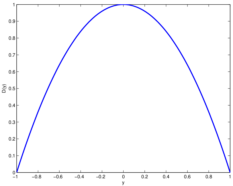
Here $\alpha_{1}\in[0,1]$ and $\alpha_{2}\in[0,1]$ , with $\alpha_{1}+\alpha_{2}\leq 1$ , measure the importance the individuals place on others opinions and actual price trend in forming expectations about future price changes. The random variables $\eta$ and $\eta_{*}$ are assumed distributed accordingly to $\Theta(\eta)$ with zero mean and variance $\sigma^{2}$ and measure individual deviations from the average behavior. The function $H(y)\in[0,1]$ is taken symmetric on the interval $I$ , and characterize the herding behavior, whereas $D(y)$ defines the diffusive behavior, and will be also taken symmetric on $I$ . Simple examples of herding function and diffusion function are given by

H(y)=a+b(1-|y|),\qquad D(y)=(1-y^{2})^{\gamma},

with $0\leq a+b\leq 1$ , $a\geq 0,b>0$ , $\gamma>0$ (see Figure 1). Other choices are of course possible, note that in order to preserve the bounds for $y$ it is essential that $D(y)$ vanishes in $y=\pm 1$ . Both functions take into account that extremal positions suffer less herding and fluctuations. For $b=0$ , $H(y)$ is constant and no herding effect is present and the mean investment propensity is preserved when the market influence is neglected ( $\alpha_{2}=0$ ) as in classical opinion models a model ( see [32] at the reference therein).

Refer to caption — Figure 1: Typical examples of herding function $H(y)$ (left) and diffusion function $D(y)$ (right).

A remarkable feature of the above relations is the presence of the normalized value function $\Phi(\dot{S}(t)/{S(t)})$ in $[-1,1]$ in the sense of Kahneman and Tversky [12, 13] that models the reaction of individuals towards potential gain and losses in the market [12]. This permits to introduce behavioral aspects in the market dynamic and to take into account the influence of psychology on the behavior of financial practitioners.

The value function is defined on deviations from a reference point, which is usually assumed equal to zero (but it can be considered also positive or negative), and is normally concave for gains (implying risk aversion), commonly convex for losses (risk seeking) and is generally steeper for losses than for gains (loss aversion)(see Figure 2).

Let us ignore for the moment the price evolution. The above binary interaction gives the following kinetic equation for the time evolution of chartists

\frac{\partial f}{\partial t}=Q(f,f),

(3)

where for any test function $\varphi$ the interaction operator $Q$ can be conveniently written in weak form as

\int_{-1}^{1}Q\varphi(y)\,dy=\int_{[-1,1]^{2}}\int_{{\mathbb{R}}^{2}}B(y,y_{*},\eta,\eta_{*})f(y)f(y_{*})(\varphi(y^{\prime})-\varphi(y))d\eta\,d\eta_{*}\,dy_{*}\,dy

(4)

with the transition rate has given by

B(y,y_{*},\eta,\eta_{*})=\Theta(\eta)\Theta(\eta_{*})\chi(|y^{\prime}|\leq 1)\chi(|y_{*}^{\prime}|\leq 1),

being $\chi(\cdot)$ the indicator function. Note that the mass density of chartists $\rho_{C}(t)$ is an invariant for the interaction, ( $\varphi\equiv 1$ ).
It is worth to observe that for a given $D_{C}(y)$ a suitable choice of the support of the random variable $\eta$ , avoids the dependence of the collisional kernel $B(y,y_{*})$ on the variables $y$ , $y^{*}$ .
As an example, if we take $D(y)=1-y^{2}$ we have

	$\displaystyle y^{\prime}$	$\displaystyle=$	$\displaystyle(1-\alpha_{1}H(y)-\alpha_{2})y+\alpha_{1}H(y)y_{*}+\alpha_{2}\Phi\left(\frac{\dot{S(t)}}{S(t)}\right)+(1-y^{2})\eta$
		$\displaystyle\leq$	$\displaystyle(1-\alpha_{1}H(y)-\alpha_{2})y+\alpha_{1}H(y)+\alpha_{2}+(1-y^{2})\eta.$

Then to have $y^{\prime}\leq 1$ for any $y\in[-1,1]$ , we have to chose $\eta$ such that

\displaystyle(1-y^{2})\eta\leq(1-\alpha_{1}-\alpha_{2})(1-y)

which gives

\eta\leq\frac{1}{2}(1-\alpha_{1}-\alpha_{2}).

Analogously we can ensure $y^{\prime}\geq-1$ , thus it is enough to take

\eta\in[-\frac{1}{2}(1-\alpha_{1}-\alpha_{2}),\frac{1}{2}(1-\alpha_{1}-\alpha_{2})].

For this reason, in the rest of the paper, we will consider only kernel of “maxwellian type”

B(y,y_{*},\eta,\eta_{*})=\Theta(\eta)\Theta(\eta_{*}).

Strategy exchange chartists-fundamentalists.

In addition to the change of investment propensity due to a balance between herding behavior and the price followers nature of chartists, the model includes the possibility that an agent changes its strategy from chartist to fundamentalists and viceversa.

Agents meet individual from the other group, compare excess profits from both strategies and with a probability depending on the pay-off differential switch to the more successful strategy. When a chartist and a fundamentalist meet they characterize the success of a given strategy trough the profits earned by comparing

X_{C}(y,t)=\psi(y)\left(\frac{\dot{S}(t)/\mu+D}{S(t)}-r\right),\quad X_{F}(t)=k\frac{|S_{F}-S(t)|}{S(t)}.

(5)

Here $\psi(y)\in[-1,1]$ has the same sign of $y$ and takes into account the change of sign in the profits accordingly to the actual behavior of the agent in the market which rely on his investment propensity $y$ . The simplest choice is $\psi(y)=\text{sgn}(y)$ .

The value $D$ is the nominal dividend and $r$ the average real return of the market, such that $r={D}/{S_{F}}$ , i.e. evaluated at its fundamental value $S_{F}$ in a state of stable price $\dot{S}=0$ the asset yield the same returns of other investments, or equivalently $X_{C}=X_{F}=0$ . The discount factor $k<1$ is justified by the observation that $X_{F}$ is an expected gain realized only after reversal to the fundamental value. Finally $\mu>0$ measures the frequency of the exchange rates.

A chartist characterized by an investment propensity $y$ and a fundamentalist meet each other, and after comparing their strategies, they exchange strategies with a rate given by a suitable monotone function $B_{FC}(\cdot)\geq 0$ . More precisely a chartist switch to fundamentalist with a rate $B_{FC}(X_{F}-X_{C})$ and a fundamentalist switch to chartist at a rate $B_{FC}(X_{C}-X_{F})$ .

For chartists we define the following linear strategy exchange operator

Q_{FC}(f)=\mu\rho_{F}(t)f(y)(B_{FC}(X_{C}-X_{F})-B_{FC}(X_{F}-X_{C}))

where $\mu>0$ measures the frequency of the exchange rates.

Taking into account such strategy exchanges we have the chartists-fundamentalists model

\left\{\begin{array}[]{lcl}\displaystyle\frac{\partial f}{\partial t}=Q(f,f)+\mu\rho_{F}(t)f(y)(B_{FC}(X_{C}-X_{F})-B_{FC}(X_{F}-X_{C}))\\[7.11317pt] \displaystyle\frac{\partial\rho_{F}}{\partial t}=\mu\rho_{F}(t)\int_{-1}^{1}f(y)(B_{FC}(X_{F}-X_{C})-B_{FC}(X_{C}-X_{F}))\,dy.\end{array}\right.

(6)

It is immediate to verify that the total number density $\rho_{C}+\rho_{F}$ is conserved in time.

Price evolution.

Finally we introduce the probability density $V(s,t)$ of a given price $s$ at time $t$ . The effective market price $S(t)$ is defined as the mean value

S(t)=\int_{0}^{\infty}V(s,t)s\,ds.

(7)

Following Lux and Marchesi [18] the microscopic dynamic of the price is given by

s^{\prime}=s+\beta(\rho_{C}t_{C}Y(t)s+\rho_{F}\gamma(S_{F}-s))+\eta s

(8)

where the parameters $\beta$ , represent the price speed evaluation, $\eta$ is a random variable with zero mean and variance $\zeta^{2}$ , distributed accordingly to $\Psi(\eta)$ . In the above relation chartists either buy or sell the same number $t_{C}$ of units and $\gamma$ is the reaction strength of fundamentalists to deviations from the fundamental value.

Thus the chartists-fundamentalists system of equations (6) is complemented with the equation for the price distribution

\frac{\partial V}{\partial t}=L(V),

(9)

where the operator $L$ , is linear, and in weak form it reads

\int_{0}^{\infty}L(V)(s)\varphi(s)\,ds=\int_{0}^{\infty}\int_{{\mathbb{R}}}b(s,\eta)V(s)(\varphi(s^{\prime})-\varphi(s))d\eta\,ds

(10)

with the transition rate $b(s,\eta)=\Psi(\eta)\chi(s^{\prime}\geq 0).$
As before, a suitable choice of the domain for the support of variable $\eta$ ensures $s^{\prime}\geq 0$ . Assuming

\eta\in[-1+\beta(\rho_{C}T_{C}+\rho_{F}\gamma),1-\beta(\rho_{C}T_{C}+\rho_{F}\gamma)],\quad\beta(\rho_{C}T_{C}+\rho_{F}\gamma)<1,

permits to express the transition rate in the simpler form

b(s,\eta)=\Psi(\eta).

Note that the expected value for the stock price satisfies the same differential equation as in[17, 18]

\frac{dS(t)}{dt}=\beta\rho_{C}t_{C}Y(t)S(t)+\beta\rho_{F}\gamma(S_{F}-S(t)).

(11)

Booms, crashes and macroscopic stationary states.

In order to study the macroscopic steady states and relate them to the value function $\Phi$ let us start by observing that the equilibrium states for the price satisfy

\rho_{C}t_{C}YS+\rho_{F}\gamma(S_{F}-S)=0

and thus fall in one of the following categories

(i)

$\rho_{F}\neq 0,\quad S=\frac{\rho_{F}\gamma S_{F}}{\rho_{F}\gamma-\rho_{C}t_{C}Y},\ \quad\rho_{F}\gamma S_{F}-\rho_{C}t_{C}Y\geq 0$ .
(ii)

$\quad\rho_{F}=0,\quad Y=0,\quad S\,{\rm arbitrary},$
(iii)

$\quad\rho_{F}=0,\quad S=0,\quad Y\,{\rm arbitrary}.$

At equilibrium we require $\rho_{F}$ , $\rho_{C}$ and $Y$ to be constants. In order for the number densities to be constants we require $Q_{FC}=0$ . For $\rho_{F}\neq 0$ and $\rho_{C}\neq 0$ , thanks to monotonicity of $B_{FC}$ , we have $X_{C}=X_{F}$ or equivalently $S=S_{F}$ . Note that $Q_{FC}$ vanishes also when $\rho_{F}=0$ or $\rho_{C}=0$ . These considerations reduce the set of possible equilibrium configurations to

(i)

$\quad\rho_{F}\neq 0,\quad S=S_{F},\quad Y=0,$
(ii)

$\quad\rho_{F}=0,\quad Y=0,\quad S\,{\rm arbitrary},$
(iii)

$\quad\rho_{F}=0,\quad S=0,\quad Y\,{\rm arbitrary}.$

Finally we consider the requirements for $Y$ to be constant. In the case $Q_{FC}=0$ the first moment equation reads

	$\displaystyle\frac{d}{dt}Y(t)=$	$\displaystyle-$	$\displaystyle\alpha_{1}\int_{-1}^{1}H(y)yf(y)dy-\alpha_{2}\rho_{C}Y(t)$
		$\displaystyle+$	$\displaystyle\alpha_{1}Y(t)\int_{-1}^{1}H(y)f(y)dy+\alpha_{2}\rho_{C}\Phi\left(\frac{\dot{S}(t)}{S(t)}\right),$

which gives the steady state condition

-\alpha_{1}\int_{-1}^{1}H(y)yf(y)dy-\alpha_{2}\rho_{C}Y+\alpha_{1}Y\int_{-1}^{1}H(y)f(y)dy+\alpha_{2}\rho_{C}\Phi\left(\frac{\dot{S}(t)}{S(t)}\right)=0.

This gives a constraint for the value function $\Phi$ , precisely

\displaystyle\alpha_{2}\rho_{C}\Phi\left(\frac{\dot{S}(t)}{S(t)}\right)=\alpha_{1}\int_{-1}^{1}H(y)yf(y)dy+\alpha_{2}\rho_{C}Y-\alpha_{1}Y\int_{-1}^{1}H(y)f(y)dy

which in the simple case of $H$ constant reduces to

\alpha_{2}\rho_{C}\left(\Phi\left(\frac{\dot{S}(t)}{S(t)}\right)-Y\right)=0.

Now using the fact that

\frac{\dot{S}(t)}{S(t)}=\beta\rho_{C}t_{C}Y(t)+\beta\rho_{F}\gamma\frac{(S_{F}-S(t))}{S(t)},

we can state

Proposition 1

The system of equations (6) in the case of $H$ constant admits the following possible equilibrium configurations

(i)

$\quad\rho_{F}\neq 0,\quad S=S_{F},\quad Y=0,\quad\Phi(0)=0$ ,
(ii)

$\quad\rho_{F}=0,\quad Y=0,\quad\Phi(0)=0,\quad S$ arbitrary,
(iii)

$\quad\rho_{F}=0,\quad Y=Y_{*}$ , with $Y_{*}=\Phi(\beta t_{C}Y_{*}),\quad S=0$ .

Note that if the reference point for the value function $\Phi(0)\neq 0$ configuration $(i)$ and $(ii)$ are not possible for a constant $H$ . This is in good agreement with the fact that an emotional perception of the market from the chartists acts as a source of instability for the market itself. In contrast configuration $(iii)$ , corresponding to a market crash, can be achieved also for $\Phi(0)\neq 0$ . The existence of a unique fixed point $Y_{*}$ has to be guaranteed by the choice of $\Phi$ , $\beta$ and $t_{C}$ . Of course if the reference point is set to zero, $\Phi(0)=0$ , we have $Y_{*}=0$ . It is easy to verify that these possible equilibrium configurations include the ones in the original Lux-Marchesi model [17].

In addition to the above equilibrium configurations the model admits several other possible asymptotic behavior in the form of booms and cycles. Some of the fundamental features of the model are summarized in the following.

Remark 1

•

Chartists alone ( $\rho_{F}=0,\rho_{C}=1$ ) influence the price through their mean propensity to invest $Y(t)$ and at the same time the price trend influences their mean propensity through the value function $\Phi(\dot{S}(t)/S(t))$ , since $\dot{S}(t)/S(t)=\beta Y(t)t_{C}$ . Thus, except for the particular shape of the value function, if the mean propensity is initially (sufficiently) positive then it will continue to grow together with the price and the opposite occurs if it is initially (sufficiently) negative.

The market goes towards a boom (exponential grow of the price) or a crash (exponential decay of the price) with

$S(0)e^{-\beta t_{C}}\leq S(t)\leq S(0)e^{\beta t_{C}},$

and agents tend to concentrate in $y=1$ and $y=-1$ respectively depending on the choices of $H$ and $\Phi$ . This is in good agreement with the price followers nature of chartists.
•

Fundamentalists alone ( $\rho_{F}=1,\rho_{C}=0$ ) influence the price through their expectation of the fundamental price. So their effect is to drive the price towards the fundamental price. For a constant fundamental price $S_{F}$ the equilibrium state reached is characterized by $S=S_{F}$ and the trend is exponential.
•

The presence of fundamentalists acts in contrast to the chartists pressure towards market booms or crashes. If their number is large enough they are capable to drive the price towards the fundamental value otherwise the chartists dynamic may dominate. In addition to booms and crashes, we have now the possibility of price cycles/oscillations around the fundamental value.

3 Fokker-Planck approximations and asymptotic behavior

Now we consider what happens at the kinetic scale. Due to the extreme difficulty to get detailed information on the asymptotic behavior of the kinetic coupled system, we will recover for both distribution functions $f$ , and $V$ , simplified Fokker-Planck models which preserve the main features of the original kinetic model. To keep notations simple, since we are mostly interested in the study of the equilibrium states we ignore the presence of the terms describing the change of strategy. However they can be easily included in the scaling described below.

For this purpose we introduce a time scaling parameter $\xi$ and define

\tau=\xi t,\quad\tilde{f}(y,\tau)=f(y,t),\quad\tilde{V}(s,\tau)=V(s,t).

(12)

To preserve the chartists dynamic in the limit, we must require that

\lim_{\alpha_{1},\xi\rightarrow 0}\frac{\alpha_{1}}{\xi}=\tilde{\alpha_{1}},\quad\lim_{\alpha_{2},\xi\rightarrow 0}\frac{\alpha_{2}}{\xi}=\tilde{\alpha_{2}},\quad\lim_{\sigma,\xi\rightarrow 0}\frac{\sigma^{2}}{\xi}=\lambda,

(13)

where $\lambda$ is a positive constant.

Similarly for the price dynamic, we assume

\lim_{\beta,\xi\rightarrow 0}\frac{\beta}{\xi}=\tilde{\beta},\quad\lim_{\zeta,\xi\rightarrow 0}\frac{\zeta^{2}}{\xi}=\nu.

(14)

Performing similar computations as in [8] (see Appendix A and B for details) we recover the following Fokker-Planck system

		$\displaystyle\displaystyle\frac{\partial\tilde{f}}{\partial\tau}+\frac{\partial}{\partial y}\left[\rho_{C}\left(\tilde{\alpha_{1}}H(y)(\tilde{Y}-y)+\tilde{\alpha_{2}}\left(\tilde{\Phi}-y\right)\right)\tilde{f}\right]\displaystyle=\frac{\lambda\rho_{C}}{2}\frac{\partial^{2}}{\partial y^{2}}({D}^{2}(y)\tilde{f}),$			(15a)
		$\displaystyle\displaystyle\frac{\partial}{\partial\tau}\tilde{V}+\frac{\partial}{\partial s}\left[\tilde{\beta}\left(\rho_{C}\tilde{Y}t_{C}s+\rho_{F}\gamma(S_{F}-s)\right)\tilde{V}\right]=\frac{\nu}{2}\frac{\partial^{2}}{\partial s^{2}}\left(s^{2}\tilde{V}\right),$			(15b)

where we used the shorthand $\tilde{\Phi}$ for $\Phi\left({\dot{\tilde{S(\tau)}}}/{\tilde{S(\tau)}}\right)$ .

For notation simplicity in the sequel we will omit the tildes in the variables $f$ , $V$ , $Y$ and $S$ .

If we now take $D(y)=1-y^{2}$ , and $H(y)=1$ we can compute explicitly the equilibrium state for chartists with a constant mean investment propensity ${Y}=Y_{*}$ as

\begin{array}[]{lcl}{f}^{\infty}(y)&=&\displaystyle C_{0}(1+y)^{-2+Y_{*}\frac{(\tilde{\alpha_{1}}+\tilde{\alpha_{2}})}{2\lambda}}(1-y)^{-2-Y_{*}\frac{(\tilde{\alpha_{1}}+\tilde{\alpha_{2}})}{2\lambda}}\exp\left(\displaystyle-\frac{(1-Y_{*}y)(\tilde{\alpha_{1}}+\tilde{\alpha_{2}})}{\lambda(1-y^{2})}\right)\end{array}

(16)

where $C_{0}=C_{0}({Y_{*},\lambda/(\tilde{\alpha_{1}}+\tilde{\alpha_{2}})})$ is such that the mass of ${f}^{\infty}$ is equal to $\rho_{C}$ . Other choices of the diffusion function originate different steady states (see [32]).

Observe that, in the case $Y_{*}\neq 0$ , the distribution is not symmetric and in the chartist population a predominant behavior arise. Otherwise when the reference point of the value function is set to zero we have a symmetric distribution with two peaks and mean value zero, and the macroscopic state of indecision is given, microscopically, by a polarization of the chartist population among two opposite kind of behaviors (see Figure 3).

In order to study the asymptotic behavior for the price we must distinguish between the case $\rho_{F}\neq 0$ and $\rho_{F}=0$ .

Let us consider first the situation in which $\rho_{F}=0$ (or equivalently $\rho_{C}=1$ ). For this purpose, we introduce the scaling

{V}(s,\tau)=\frac{1}{s}{v}(\chi,\tau),\ \ \ \chi=\log(s).

It is straightforward to show that ${v}(\chi,\tau)$ satisfies the following linear convection diffusion equation

\frac{\partial}{\partial\tau}{v}(\chi,\tau)=\left[\frac{\nu}{2}-\tilde{\beta}Yt_{C}\right]\frac{\partial}{\partial\chi}{v}(\chi,\tau)+\frac{\nu}{2}\frac{\partial^{2}}{\partial\chi^{2}}{v}(\chi,\tau),

which admits the self-similar solution [8]

{v}(\chi,\tau)=\frac{1}{(2\log(E(\tau)/S(\tau)^{2})\pi)^{\frac{1}{2}}}\exp\left(-\frac{(\chi+\log(\sqrt{E(\tau)}/S(\tau))-\log(S(\tau)))^{2}}{2\log(E(\tau)/S(\tau)^{2})}\right),

with

E(\tau)=\int_{0}^{\infty}V(s,\tau)s^{2}\,ds.

Then reverting to the original variables it gives the lognormal behavior

{V}(s,\tau)=\frac{1}{s(2\log(E(\tau)/S(\tau)^{2})\pi)^{\frac{1}{2}}}\exp\left(-\frac{(\log(s\sqrt{E(\tau)}/S(\tau)^{2})^{2}}{2\log(E(\tau)/S(\tau)^{2})}\right),

(17)

where $E(\tau)$ satisfies the differential equation

\frac{dE}{d\tau}=(2\tilde{\beta}Yt_{C}+\nu)E(\tau).

Thus for a steady state characterized by $(ii)$ in Proposition 1 we have $S(\tau)=S_{0}$ , $Y=0$ and $E(\tau)=e^{\nu\tau}E_{0}$ .

Besides the above equilibrium state, equation (17) characterizes also the self-similar behavior of the price distribution in the case of booms and crashes, when the price $S(\tau)$ grows arbitrary or decays to zero. In particular in the limit $S(\tau)\to 0$ , point $(iii)$ in Proposition 1, the distribution function $V(s,\tau)$ concentrates near zero.

Finally we consider the microscopic behavior of the model where both $\rho_{C}\neq 0$ and $\rho_{F}\neq 0$ .

Recall now the Fokker-Planck equation for the price (15b) and consider the stationary case $(i)$ in Proposition 1. The Fokker-Planck equation in such case reads

\frac{\partial}{\partial\tau}{V}+\frac{\partial}{\partial s}\left[\tilde{\beta}\rho_{F}\gamma(S_{F}-s){V}\right]=\frac{\nu}{2}\frac{\partial^{2}}{\partial s^{2}}\left(s^{2}{V}\right).

(18)

In this case the steady state can be computed as [1, 7] and yelds

{V}^{\infty}(s)=C_{1}(\mu)\frac{1}{s^{1+\mu}}e^{-\frac{(\mu-1)S_{F}}{s}},

(19)

where $\mu=1+2\tilde{\beta}\rho_{F}\gamma/\nu$ and $C_{1}(\mu)=((\mu-1)S_{F})^{\mu}/\Gamma(\mu)$ with $\Gamma(\cdot)$ being the usual Gamma function. Therefore the stationary state is described by a Gamma-like distribution with Pareto power law tails.

Remark 2

•

The presence of fundamentalists is then essential in order to obtain fat tails in the price distribution. Their presence force the price to approach the mean value $S_{F}$ in a way similar to the redistribution of wealth in the models proposed in [1, 7]. This feature seems to be essential for the development of power law behaviors. The stationary state for the price (19) has in fact the same structure of the stationary states for the wealth in [1, 7].

•

In our description we have considered a constant value for the fundamental price. Such an assumption might seem quite unrealistic since, according to the economic literature, the fundamental price is usually treated like a temporal series with a stationary lognormal distribution. This reflect the facts that the returns in logarithmic form are gaussian distributed with zero mean and a fixed variance, i.e big jumps between two successive realizations are rarely verified. Note however that introducing a given time dependent distribution function $V_{SF}(q,t)$ for the fundamental price such that

S_{F}(t)=\int_{0}^{+\infty}V_{SF}(q,t)q\,dq,

and considering the following dynamic in the price evolution

s^{\prime}=s+\beta(\rho_{C}t_{C}Y(t)s+\rho_{F}\gamma(q-s))+\eta s,

where $s$ and $q$ are random variables distributed as $V(s,t)$ and $V_{SF}(q,t)$ , we recover

\int_{0}^{\infty}L(V)(s)\varphi(s)\,ds=\int_{0}^{\infty}\int_{0}^{\infty}\int_{{\mathbb{R}}}b(s,\eta)V_{SF}(q)V(s)(\varphi(s^{\prime})-\varphi(s))d\eta\,ds\,dq

which is the analogous of (10) and yields the same Fokker-Planck equation (15b) for the asymptotic behavior of the model. We omit the details.

4 Numerical examples

In this section we considered different numerical simulations of the kinetic system. A Monte Carlo method analogous to the one used in classical rarefied gas dynamic has been used for the simulations [2]. In order to compute the kinetic behavior of the price, we use a set of $N_{s}=50000$ samples which can be though as possible realizations of the random variable $s$ denoting the price. Since at the initial time the stock price $S_{0}$ is supposed to be known, all samples are initialized at the same value initially. We represent the initial chartists distribution with a set of $N_{c}=\rho_{C}(0)N$ sample agents with $N=50000$ . These do not represent real agents but simply statistical realization of the random variable $y$ . Such choices of $N_{s}$ and $N$ permits to obtain results with a moderate effect of fluctuations without averaging.
In all our computations we take the value function

\Phi(x)=\left\{\begin{array}[]{ll}\left(\frac{x-R_{0}}{L-R_{0}}\right)^{r},&L>x>R_{0},\\ -\left(\frac{R_{0}-x}{R_{0}+L}\right)^{l},&-L<x\leq R_{0},\\ \end{array}\right.

where $x\in[-L,L]$ , $R_{0}$ is the reference point and $0<l\leq r<1$ . For example we choose $r=1/2$ and $l=1/4$ .

Test 1

In the first test we consider the case with $\rho_{F}=0$ i.e only chartists are present in the model. We computed the equilibrium distribution for $\Phi(0)=0$ of the investment propensity. We take $\beta=0.1$ , $t_{C}=1$ , a constant herding function $H(y)=1$ and the coefficients $\alpha_{1}=\alpha_{2}=0.01$ . The initial data for the chartists is perfectly symmetric with $Y=0$ , so the price remains constant $S=S_{0}$ with $S_{0}=10$ . A particular care is required in the simulation to keep $Y=0$ since the equilibrium point is unstable and as soon as $Y\neq 0$ the results deviate towards a market boom or crash.

After $T=1500$ iteration the solution for the investment propensity has reached a stationary state and is plotted together with the solution of the Fokker-Planck limit in Figure 4. In the same figure we report also the computed solution for the price distribution and the self-similar lognormal solution of the corresponding Fokker-Planck equation. A very good agreement between the computed Boltzmann solution and the Fokker-Planck solution is observed.

Test 2

In the second test case we considered the most interesting situation with the presence of fundamentalists, i.e both chartists and fundamentalists interact in the stock market. We compute an equilibrium situation where $\rho_{F}=\rho_{C}=0.5$ and the price stationary at the fundamental value $S_{F}=20$ . We take $\beta=0.1$ , $t_{C}=1$ , $\gamma=1.3$ , $\alpha_{1}=\alpha_{2}=0.01$ . We report the result of the simulation for the price distribution at the stationary state. In Figure 5 we show the price distribution together with the steady state of the corresponding Fokker-Planck equation. The emergence of a power law is clear also for the Boltzmann model, and deviations of the two models is observed for small values of the price.

Test 3

In the third test we consider the case with strategy exchange between the two populations of interacting agents. The switching rate used to run the simulation has the following form

B_{FC}(x)=e^{\sigma x},

where $\sigma$ represent the inertia of the reaction to profit differentials. We start the simulation considering $\rho_{C}=\rho_{F}=0.5$ . The fundamental price is $S_{F}=20$ , we take $\beta=6$ , $t_{C}=0.02$ , $\gamma=0.1$ , $\sigma=0.8$ , $\mu=0.2$ , $D=0.004$ , $k=0.75$ , and $\psi(y)=\text{sgn}(y)$ . Furthermore we consider an herding function of the form $H(y)=(1-|y|)$ . We run different simulations for $T=2000$ iterations, with different values of $\alpha_{1}$ , and $\alpha_{2}$ , which measures respectively the herding and the market influence on the chartists. Three fundamental behaviors can be observed. The predominance of chartists, which leads the market towards a crash or a boom (see Figure 6), the predominance of fundamentalists, which originates damped oscillation of the price towards the fundamental value (see Figure 7), and a balanced behavior, characterized by periods with oscillation of the price around the fundamental value (see Figures 8 and 9). From the simulations it is observed that, if we start with a balanced population between chartists and fundamentalists, the parameter $\alpha_{2}$ , which characterize the influence of the price trend on the chartists investment propensity, plays a determinant role in the competition between the two different trading strategies. In particular when $\alpha_{2}\geq 0.6$ fundamentalists are predominant and price oscillations become dumped.

5 Conclusion

We derived an interacting agents kinetic model for a simple stock market characterized by two different market strategies, chartists and fundamentalists. The kinetic system couples a description for the propensity to invest of chartists and the price formation mechanism. The model is able to describe several market phenomena like the presence of of booms, crashes, and cyclic oscillations of the market price. The equilibrium behavior has been studied in a suitable asymptotic regime which originates a system of Fokker-Planck equation for the chartist’s opinion dynamics and the price formation. We found that in a system of agents acting only using a chartist strategy the distribution of price converges towards a lognormal distribution. This is in good agreement with what previously found in [8] and observed in [16]. When a second strategy based on a fundamentalist approach is introduced in the model the prices distribution displays Pareto power law tails, which is in accordance to what observed in the real market data. In the description of the chartists behavior we also introduced a value function which takes into account the effect of some psychological factors in the opinion formation dynamic. The main effect is to introduce market instabilities and to reduce the number of stable equilibrium configurations of the system. Let us finally conclude by observing that in principle several generalizations are possible. We mention here the possibility to include multiple interacting strategies and/or the influence of the wealth as an independent variable in the market dynamics.

Appendix A Fokker-Planck asymptotics for the agents distribution

We report in this appendix the details of the derivation of the Fokker-Planck equation (15a) for the distribution of chartists. Following [32] first we recall the definition of weak solution for kinetic equations of the form (3) and (9). Let $I=[-1,1]$ and $\textit{M}_{p}(I)=\left\{\varTheta\in\textit{M}_{p}:\int_{I}|y|^{p}d\varTheta(y)<+\infty\right\}$ be the space of all Borel measure of finite $p$ -th order momentum, equipped with the topology of weak convergence of the measures. Let $\textit{F}_{s}(I)$ be the class of all real functions $h$ on $I$ such that $h(\pm 1)=h^{\prime}(\pm 1)=0$ and $h^{(m)}(y)$ is Hölder continuous of order $\delta$

\|h^{(m)}\|_{\delta}=\sup_{y_{1}\neq y_{2}}\frac{|h^{(m)}(y_{1})-h^{m}(y_{2})|}{|y_{1}-y_{2}|^{\delta}}<\infty

(20)

where $0<\delta\leq 1$ , $m+\delta=s$ and $h^{(m)}$ denotes the $m$ -th derivative of $h$ .

Definition 1

Let $f^{0}(y)\in\ \textit{M}_{p}(I)$ with $p>1$ an initial probability density, a weak solution for (3) is any probability density $f\in C^{1}({\mathbb{R}}^{+},\textit{M}_{p}(I))$ satisfying

\displaystyle\frac{d}{dt}\int_{I}f(y,t)\phi(y)dy=\int_{I^{2}}\int_{{\mathbb{R}}^{2}}B(y,y_{*},\eta,\eta_{*})f(y)f(y_{*})(\phi(y^{\prime})-\phi(y))d\eta d\eta_{*}dy_{*}dy

(21)

for $t>0$ and all $\phi\in\textit{F}_{p}(I)$ , and such that

\lim_{t\rightarrow 0}\int_{I}f(y,t)\phi(y)dy=\int_{I}f^{0}(y)\phi(y)dy.

The scaled density $\tilde{f}(y,\tau)$ defined in (12) satisfies the equation in weak form

\displaystyle\frac{d}{d\tau}\int_{I}\tilde{f}(y,\tau)\phi(y)dy=\frac{1}{\xi}\int_{I^{2}}\int_{J^{2}}\Theta(\eta)\Theta(\eta_{*})\tilde{f}(y)\tilde{f}(y_{*})(\phi(y^{\prime})-\phi(y))d\eta d\eta_{*}dy_{*}dy,

(22)

where $J\subseteq{\mathbb{R}}$ is a suitable symmetric support for the random variable $\eta$ which avoids the dependence of the kernel $B$ on the variables $y$ and $y_{*}$ .

Given $\delta\geq 0$ let us take $\phi\in\textit{F}_{2+\delta}(I)$ .
From the microscopic dynamic of chartists we have

y^{\prime}-y=\alpha_{1}H(y)(y-y_{*})+\alpha_{2}(\tilde{\Phi}-y)+D(y)\eta.

In the asymptotic limit $\xi\rightarrow 0$ , $\sigma^{2}\rightarrow 0$ , we have $y-y^{\prime}\sim 0$ and we can use the Taylor expansion

	$\displaystyle\phi(y^{\prime})-\phi(y)=\left(\alpha_{1}H(y)(y-y_{*})+\alpha_{2}(\tilde{\Phi}-y)+D(y)\eta\right)\phi^{\prime}(y)$
	$\displaystyle+\frac{1}{2}\left(\alpha_{1}H(y)(y-y_{*})+\alpha_{2}(\tilde{\Phi}-y)+D(y)\eta\right)^{2}\phi^{\prime\prime}(\tilde{y}),$

where, for some $0\leq\theta\leq 1$

\tilde{y}=\theta y^{\prime}+(1-\theta)y.

Inserting this expansion in the weak formulation of the Boltzman equation, we get

		$\displaystyle\displaystyle\frac{d}{d\tau}$	$\displaystyle\int_{I}\tilde{f}(y,\tau)\phi(y)dy=$
		$\displaystyle\displaystyle\frac{1}{\xi}$	$\displaystyle\int_{I^{2}}\int_{J^{2}}\Theta(\eta)\Theta(\eta_{})\left[\left(\alpha_{1}H(y)(y-y_{})+\alpha_{2}(\tilde{\Phi}-y)+D(y)\eta\right)\phi^{\prime}(y)\right.$
		$\displaystyle+$	$\displaystyle\left.\frac{1}{2}\left(\alpha_{1}H(y)(y-y_{})+\alpha_{2}(\tilde{\Phi}-y)+D(y)\eta\right)^{2}\phi^{\prime\prime}(y)\right]\tilde{f}(y)\tilde{f}(y_{})d\eta d\eta_{}dy_{}dy$
		$\displaystyle+$	$\displaystyle R(\xi,\sigma)$

where

	$\displaystyle R(\xi,\sigma)$	$\displaystyle=$	$\displaystyle\frac{1}{2\xi}\int_{I^{2}}\int_{J^{2}}\Theta(\eta)\Theta(\eta_{})\left(\alpha_{1}H(y)(y-y_{})+\alpha_{2}(\tilde{\Phi}-y)+D(y)\eta\right)^{2}$
		$\displaystyle\cdot$	$\displaystyle(\phi^{\prime\prime}(\tilde{y})-\phi^{\prime\prime}(y))\tilde{f}(y)\tilde{f}(y_{})d\eta_{}d\eta dy_{*}dy.$

In order to prove that the remainder () goes to zero as $\xi\to 0$ we start observing that, being $\phi\in\textit{F}_{2+\delta}(I)$ , and $|\tilde{y}-y|=\theta|y^{\prime}-y|$ we get

|\phi^{\prime\prime}(\tilde{y})-\phi^{\prime\prime}(y)|\leq\|\phi^{\prime\prime}\|_{\delta}|\tilde{y}-y|^{\delta}\leq\|\phi^{\prime\prime}\|_{\delta}|y^{\prime}-y|^{\delta}.

Hence

	$\displaystyle\displaystyle\|R(\xi,\sigma)\|$	$\displaystyle\leq$	$\displaystyle\frac{\\|\phi^{\prime\prime}\\|_{\delta}}{2\xi}\int_{I^{2}}\int_{J^{2}}\Theta(\eta)\Theta(\eta_{*})\cdot$
		$\displaystyle\cdot$	$\displaystyle\left\|\alpha_{1}H(y)(y-y_{})+\alpha_{2}(\tilde{\Phi}-y)+D(y)\eta\right\|^{2+\delta}\tilde{f}(y)\tilde{f}(y_{})d\eta_{}d\eta dy_{}dy.$

Using the fact that $|H(y)|\leq 1$ , $|\tilde{\Phi}|\leq 1$ , $|y|\leq 1$ and applying the following simple inequality

\displaystyle\displaystyle\left|\alpha_{1}H(y)(y-y_{*})+\alpha_{2}(\tilde{\Phi}-y)+D(y)\eta\right|^{2+\delta}\leq C_{\delta}\left(\alpha_{1}^{2+\delta}+\alpha_{2}^{2+\delta}+|\eta|^{2+\delta}\right)

with $C_{\delta}$ a suitable positive constant, we finally obtain

|R(\xi,\sigma)|\leq C_{\delta}\rho_{C}^{2}\frac{\|\phi^{\prime\prime}\|_{\delta}}{2\xi}\left(\alpha_{1}^{2+\delta}+\alpha_{2}^{2+\delta}+\int_{J}\Theta(\eta)|\eta|^{2+\delta}d\eta\right).

To simplify computations, we assume that $\Theta$ , with zero mean and variance $\lambda\xi$ , is the density of $\sqrt{\lambda\xi}W$ , where $W$ is a random variable with zero mean and unit variance, that belongs to $\textit{M}_{2+\alpha}$ , for $\alpha>\delta$ , so we have

\int_{J}\Theta(\eta)|\eta|^{2+\delta}d\eta=E\left(\left|\sqrt{\lambda\xi}W\right|^{2+\delta}\right)=(\lambda\xi)^{1+\frac{\delta}{2}}E\left(|W|^{2+\delta}\right),

and $E\left(|W|^{2+\delta}\right)$ is bounded. This is enough to show that in the asymptotic limit defined by (13) the quantity $R(\xi,\sigma)$ tends to zero.

Finally taking the limit in the weak formulation yields

$\displaystyle\lim_{\xi\to 0}$	$\displaystyle\displaystyle\frac{1}{\xi}\int_{I^{2}}\int_{J^{2}}$	$\displaystyle\Theta(\eta)\Theta(\eta_{})\left[\left(\alpha_{1}H(y)(y-y_{})+\alpha_{2}(\tilde{\Phi}-y)+D(y)\eta\right)\phi^{\prime}(y)\right.$
	$\displaystyle+$	$\displaystyle\left.\frac{1}{2}\left(\alpha_{1}H(y)(y-y_{})+\alpha_{2}(\tilde{\Phi}-y)+D(y)\eta\right)^{2}\phi^{\prime\prime}(y)\right]\tilde{f}(y)\tilde{f}(y_{})d\eta d\eta_{}dy_{}dy$
	$\displaystyle=$	$\displaystyle\int_{I}\left[-\left(\rho_{C}\tilde{\alpha_{1}}H(y)(Y-y)+\rho_{C}\tilde{\alpha_{2}}(\tilde{\Phi}-y)\right)\phi^{\prime}(y)+\frac{\lambda}{2}(\rho_{C}{D}^{2}(y))\phi^{\prime\prime}(y)\right]\tilde{f}(y)dy,$

which is nothing but the weak form of the Fokker-Planck equation (15a). We can then state the following theorem

Theorem 1

Let the probability density $f^{0}\in{M}_{0}(I)$ , and let the symmetric density $\Theta$ be in $M_{2+\alpha}$ with $\alpha>\delta$ . Then in the asymptotic limit defined by (13) the weak solution to the Boltzmann equation (22) for the scaled density $\tilde{f}(y,\tau)$ converges, up to extraction of a subsequence, to the weak solution of the Fokker-Planck equation (15a).

Appendix B Fokker-Planck asymptotics for the price distribution

In this appendix we derive the Fokker-Planck limit (15b) for the scaled density distribution of the price. Now let $\textit{F}_{s}({\mathbb{R}}^{+})$ be the class of all real functions $h$ on ${\mathbb{R}}$ such that $h(0)=h^{\prime}(0)=0$ and $h^{m}(y)$ is Hölder continuous of order $\delta$ . We have the following

Definition 2

Given an initial price distribution $V_{0}(s)\in\textit{M}_{p}({\mathbb{R}}^{+})$ with $p>1$ a weak solution to (9) is any probability density $V\in C^{1}({\mathbb{R}}^{+},\textit{M}_{p}({\mathbb{R}}^{+}))$ satisfying

\displaystyle\frac{d}{dt}\int_{{\mathbb{R}}^{+}}V(s,t)\phi(s)ds=\int_{{\mathbb{R}}^{+}}\int_{{\mathbb{R}}}b(s,\eta)V(s,t)(\phi(s^{\prime})-\phi(s))d\eta ds

(24)

for $t>0$ and all $\phi\in\textit{F}_{p}({\mathbb{R}}^{+})$ and such that

\lim_{t\rightarrow 0}\int_{{\mathbb{R}}^{+}}V(s,t)\phi(s)ds=\int_{{\mathbb{R}}^{+}}\phi(s)V_{0}(s)ds.

Again we start with the weak formulation which now reads

\frac{d}{d\tau}\int_{{\mathbb{R}}^{+}}\tilde{V}(s,\tau)\phi(s)ds=\frac{1}{\xi}\int_{{\mathbb{R}}^{+}}\int_{K}\Psi(\eta)\tilde{V}(s)(\phi(s^{\prime})-\phi(s))d\eta ds,

(25)

where $K\subseteq{\mathbb{R}}$ is a suitable symmetric support for the random variable $\eta$ which avoids the dependence of the kernel $b$ on the variable $s$ .

Let us take $\phi\in\textit{F}_{2+\delta}({\mathbb{R}}^{+})$ with $\delta>0$ . Using a Taylor expansion of $\phi$ around $s$

	$\displaystyle\phi(s^{\prime})-\phi(s)$	$\displaystyle=$	$\displaystyle\left(\beta(\rho_{C}t_{C}Ys+\rho_{F}\gamma(S_{F}-s))+\eta s\right)\phi^{\prime}(s)$
		$\displaystyle+$	$\displaystyle\frac{1}{2}\left(\beta(\rho_{C}t_{C}Ys+\rho_{F}\gamma(S_{F}-s))+\eta s\right)^{2}\phi^{\prime\prime}(\tilde{s}),$

where for some $0\leq\theta\leq 1$

\tilde{s}=\theta s^{\prime}+(1-\theta)s,

and substituting into (25) we have

$\displaystyle\frac{d}{d\tau}\int_{{\mathbb{R}}^{+}}\tilde{V}(s,\tau)\phi(s)ds$	$\displaystyle=$	$\displaystyle\frac{1}{\xi}\int_{{\mathbb{R}}^{+}}\int_{K}\Psi(\eta)[\left(\beta(\rho_{C}t_{C}Ys+\rho_{F}\gamma(S_{F}-s))+\eta s\right)\phi^{\prime}(s)$
	$\displaystyle+$	$\displaystyle\frac{1}{2}\left(\beta(\rho_{C}t_{C}Ys+\rho_{F}\gamma(S_{F}-s))+\eta s\right)^{2}\phi^{\prime\prime}(s)]\tilde{V}(s)d\eta ds$
	$\displaystyle+$	$\displaystyle R(\beta,\zeta,\xi)$

where

\displaystyle R(\beta,\zeta,\xi)

\displaystyle=

\displaystyle\frac{1}{2\xi}\int_{{\mathbb{R}}^{+}}\int_{K}\Psi(\eta)\left(\beta(\rho_{C}t_{C}Ys+\rho_{F}\gamma(S_{F}-s))+\eta s\right)^{2}\cdot(\phi^{\prime\prime}(\tilde{s})-\phi^{\prime\prime}(s))\tilde{V}(s)d\eta ds.

Analogously as before, in order to perform the asymptotic limit we need to show that the quantity $R(\beta,\zeta,\xi)$ approaches zero as $\xi\to 0$ . We observe that being $\phi\in F_{2+\delta}({\mathbb{R}}+)$ and $|\tilde{s}-s|=\theta|s^{\prime}-s|$ we have

|\phi^{\prime\prime}(\tilde{s})-\phi^{\prime\prime}(s)|\leq\|\phi^{\prime\prime}\|_{\delta}|s^{\prime}-s|^{\delta}

hence

\displaystyle|R(\beta,\zeta,\xi)|\leq\frac{\|\phi^{\prime\prime}\|_{\delta}}{2\xi}\int_{{\mathbb{R}}^{+}}\int_{K}\Psi(\eta)\left|\beta\left(\rho_{C}t_{C}Y+\rho_{F}\gamma\frac{(S_{F}-s)}{s}\right)+\eta\right|^{2+\delta}s^{2+\delta}\tilde{V}(s)d\eta ds.

Next we observe that

	$\displaystyle\left\|\beta\left(\rho_{C}t_{C}Y+\rho_{F}\gamma\frac{(S_{F}-s)}{s}\right)+\eta\right\|^{2+\delta}\leq$
			(26)
	$\displaystyle C_{2+\delta}\left((\beta\rho_{C}t_{C})^{2+\delta}+(\beta\rho_{F}\gamma)^{2+\delta}\left(\frac{S_{F}^{2+\delta}+s^{2+\delta}}{s^{2+\delta}}\right)+\|\eta\|^{2+\delta}\right),$

where $C_{2+\delta}>0$ is a suitable constant.

As in appendix A we assume that $\Psi$ , with zero mean and variance $\nu\zeta$ is the density of $\sqrt{\nu\zeta}W$ , where $W$ is a random variable with zero mean and unit variance, that belongs to $\textit{M}_{2+\alpha}$ , for $\alpha>\delta$ , so we have

\int_{K}\Psi(\eta)|\eta|^{2+\delta}d\eta=E\left(\left|\sqrt{\nu\zeta}W\right|^{2+\delta}\right)=(\nu\zeta)^{1+\frac{\delta}{2}}E\left(|W|^{2+\delta}\right),

(27)

and $E\left(|W|^{2+\delta}\right)$ is bounded.

Then we obtain

	$\displaystyle\|R(\beta,\zeta,\xi)\|$	$\displaystyle\leq$	$\displaystyle C_{2+\delta}\frac{\\|\phi^{\prime\prime}\\|_{\delta}}{2\xi}\left\{\left[(\beta\rho_{C}t_{C})^{2+\delta}+(\beta\rho_{F}\gamma)^{2+\delta}+(\nu\zeta)^{1+\frac{\delta}{2}}E\left(\|W\|^{2+\delta}\right)\right]\right.$
		$\displaystyle\cdot$	$\displaystyle\left.\int_{{\mathbb{R}}^{+}}s^{2+\delta}\tilde{V}(s)ds+(\beta\rho_{F}\gamma)^{2+\delta}S_{F}^{2+\delta}\right\}.$

From this inequality it follows that $R(\beta,\zeta,\xi)$ tends to zero in the limit (14) if

\displaystyle\int_{{\mathbb{R}}^{+}}\tilde{V}(s,\tau)s^{2+\delta}ds

is bounded at any fixed time $\tau>0$ , provided that the same bound holds at time $\tau=0$ .

To show this we start again from the weak formulation (25). The choice $\phi(y)=y^{p}$ gives

\frac{d}{d\tau}\int_{{\mathbb{R}}^{+}}\tilde{V}(s)s^{p}ds=\frac{1}{\xi}\int_{{\mathbb{R}}^{+}}\int_{K}\Psi(\eta)\tilde{V}(s)(s^{\prime p}-s^{p})d\eta ds.

Now

s^{\prime p}-s^{p}=ps^{p-1}(s^{\prime}-s)+\frac{1}{2}p(p-1)\tilde{s}^{p-2}(s^{\prime}-s)^{2}

where for some $0\leq\theta\leq 1$

\tilde{s}=\theta s^{\prime}+(1-\theta)s.

Recalling the microscopic dynamic for the evolution of the price variable $s$ we can write

$\displaystyle\displaystyle\frac{d}{d\tau}\int_{{\mathbb{R}}^{+}}\tilde{V}(s)s^{p}ds$	$\displaystyle=$	$\displaystyle\frac{1}{\xi}\int_{{\mathbb{R}}^{+}}\int_{K}\Psi(\eta)\tilde{V}(s)\left[ps^{p-1}(s^{\prime}-s)+\frac{1}{2}p(p-1)\tilde{s}^{p-2}(s^{\prime}-s)^{2}\right]d\eta ds$
	$\displaystyle=$	$\displaystyle\displaystyle\frac{p}{\xi}\int_{{\mathbb{R}}^{+}}\int_{K}\Psi(\eta)\tilde{V}(s)s^{p-1}\left[\left(\beta(\rho_{C}t_{C}Ys+\rho_{F}\gamma(S_{F}-s)\right)+\eta s\right]d\eta ds$
	$\displaystyle+$	$\displaystyle\displaystyle\frac{p(p-1)}{2\xi}\int_{{\mathbb{R}}^{+}}\int_{K}\Psi(\eta)\tilde{V}(s)\tilde{s}^{p-2}\left[\beta\left(\rho_{C}t_{C}Ys+\rho_{F}\gamma{(S_{F}-s)}\right)+\eta s\right]^{2}d\eta ds.$

Since the random variable $\eta$ has zero mean value, the first term in the last expression reduces to

p\frac{\beta}{\xi}\left[\left(\rho_{C}t_{C}Y-\rho_{F}\gamma\right)\int_{{\mathbb{R}}^{+}}\tilde{V}(s)s^{p}ds+\rho_{F}S_{F}\gamma\int_{{\mathbb{R}}^{+}}\tilde{V}(s)s^{p-1}ds\right].

For the second therm, we know that

	$\displaystyle\displaystyle\tilde{s}$	$\displaystyle=$	$\displaystyle\theta(s+\beta(\rho_{C}t_{C}Ys+\rho_{F}\gamma(S_{F}-s))+\eta s)+(1-\theta)s$
		$\displaystyle=$	$\displaystyle\displaystyle s\left[\theta\beta\left(\rho_{C}t_{C}Y+\rho_{F}\gamma\frac{(S_{F}-s)}{s}\right)+\theta\eta+1\right],$

which implies

\displaystyle\tilde{s}^{p-2}

\displaystyle\leq

\displaystyle{\bar{C}}_{p}\left[(\beta\rho_{C}t_{C})^{p-2}+(\beta\rho_{F}\gamma)^{p-2}\left(\frac{S_{F}^{p-2}+s^{p-2}}{s^{p-2}}\right)+|\eta|^{p-2}+1\right]s^{p-2},

with ${\bar{C}}_{p}$ a suitable constant.

Gathering all this the weak formulation gives

$\displaystyle\displaystyle\frac{d}{d\tau}\int_{{\mathbb{R}}^{+}}\tilde{V}(s)s^{p}ds$	$\displaystyle\leq$	$\displaystyle p\frac{\beta}{\xi}\left[\left(\rho_{C}t_{C}Y-\rho_{F}\gamma\right)\int_{{\mathbb{R}}^{+}}\tilde{V}(s)s^{p}ds+\rho_{F}S_{F}\gamma\int_{{\mathbb{R}}^{+}}\tilde{V}(s)s^{p-1}ds\right]$
	$\displaystyle+$	$\displaystyle\frac{p(p-1)}{2\xi}{\bar{C}_{p}}\int_{{\mathbb{R}}^{+}}\int_{K}\Psi(\eta)\tilde{V}(s)s^{p}\left[\beta\left(\rho_{C}t_{C}Y+\rho_{F}\gamma\frac{(S_{F}-s)}{s}\right)+\eta\right]^{2}$
	$\displaystyle\cdot$	$\displaystyle\left[(\beta\rho_{C}t_{C})^{p-2}+(\beta\rho_{F}\gamma)^{p-2}\left(\frac{S_{F}^{p-2}+s^{p-2}}{s^{p-2}}\right)+\|\eta\|^{p-2}+1\right]d\eta ds.$

Now if we consider the asymptotic limit (14) and recall (27) for the high order moments of $\eta$ , it follows that the $p$ -moments of $\tilde{V}(s,\tau)$ are bounded at any finite time independently of $\xi$ and for $p\geq 2+\delta$ satisfy

\displaystyle\displaystyle\frac{d}{d\tau}\int_{{\mathbb{R}}^{+}}\tilde{V}(s)s^{p}ds\leq A_{p}\int_{{\mathbb{R}}^{+}}V(s,t)s^{p}ds+B_{p}\int_{{\mathbb{R}}^{+}}V(s,t)s^{p-1}ds

where $A_{p}=p\tilde{\beta}\left(\rho_{C}t_{C}Y-\rho_{F}\gamma\right)+{p(p-1)}{\nu\bar{C}_{p}}/2$ and $B_{p}=p\tilde{\beta}\rho_{F}S_{F}\gamma$ .
Coming back to the asymptotic expansion we can finally perform the limit

$\displaystyle\lim_{\xi\to 0}$	$\displaystyle\displaystyle\frac{1}{\xi}\int_{{\mathbb{R}}^{+}}\int_{K}$	$\displaystyle\Psi(\eta)\left[\frac{}{}\left(\beta(\rho_{C}(t)Yt_{C}s+\rho_{F}\gamma(S_{F}-s))+\eta s\right)\phi^{\prime}(s)\right.$
	$\displaystyle+$	$\displaystyle\left.\frac{1}{2}\left(\beta(\rho_{C}(t)Yt_{C}s+\rho_{F}\gamma(S_{F}-s))+\eta s\right)^{2}\phi^{\prime\prime}(s)\right]\tilde{V}(s)d\eta ds$
	$\displaystyle=$	$\displaystyle\int_{{\mathbb{R}}^{+}}\left[\tilde{\beta}(\rho_{C}(t)Yt_{C}s\rho_{F}\gamma(S_{F}-s))\phi^{\prime}(s)+\frac{\nu}{2}s^{2}\phi^{\prime\prime}(s)\right]\tilde{V}(s)ds,$

which is the weak form of the Fokker-Planck equation for the price (15b). So we proved the following

Theorem 2

Let the probability density $V_{0}\in{M}_{0}({\mathbb{R}}^{+})$ . Then in the limit defined by (14) the weak solution to the Boltzmann equation (25) for the scaled density $\tilde{V}(s,\tau)$ converges, up to extraction of a subsequence, to a weak solution of $(\ref{8b})$ .

References

[1] Bouchaud, J.P., Mézard, M., Wealth condensation in a simple model of economy, Physica A, 282, (2000), 536–.
[2] Cercignani, C., Illner, R., Pulvirenti, M., The mathematical theory of dilute gases. Springer, New-York (1994)
[3] Chakraborti, A., Chakrabarti, B.K., Statistical mechanics of money: how saving propensity affects its distributions, Eur. Phys. J. B., 17, (2000), 167–.
[4] Chatterjee, A., Chakrabarti, B.K., Manna, S.S., Pareto law in a kinetic model of market with random saving propensity, Phys. A 335, (2004), 155–163.
[5] Cont, B., Bouchaud, J. P., Herd behaviour and aggregate fluctuations in financial markets. Macroeconomic Dynamics, 4, (2000), 170–196.
[6] Cordier, S., Maldarella, D., Pareschi, L., Piatecki, C. Microscopic and kinetic models in financial markets. Mathematical Modelling of Collective Behavior in Socio-Economic and Life Sciences, Birkhauser (to appear).
[7] Cordier, S., Pareschi L., Toscani G., On a kinetic model for a simple market economy. J. Stat. Phys., 120, (2005), 253–277.
[8] Cordier, S., Pareschi L., Piatecki C., Mesoscopic modelling of financial markets. J. Stat. Phys., 134, (2009), 161–184.
[9] Drǎgulescu, A., Yakovenko, V.M., Statistical mechanics of money, Eur. Phys. J. B., 17, (2000), 723–729.
[10] Düring, B., Toscani, G., Hydrodynamics from kinetic models of conservative economies, Physica A, 384, (2007), 493–506.
[11] Gabaix, X., Gopikrishnan, P., Plerou, V., Stanley, H.E., A Theory of Power-Law Distributions in Financial Market Fluctuations, Nature 423, (2003), 267–270.
[12] Kahneman, D., Tversky, A., Prospect Theory: An Analysis of Decision under Risk, Econometrica, (1979), 263–292.
[13] Kahneman, D., Tversky, A., Choices, Values, and Frames. Cambridge: Cambridge University Press, (2000).
[14] Ispolatov, S., Krapivsky, P.L., Redner, S., Wealth distributions in asset exchange models, Eur. Phys. J. B, 2, (1998), 267–276.
[15] Levy, M., Levy, H., Solomon, S., A microscopic model of the stock market: Cycles, booms and crashes, Economics Letters, 45, (1994), 103–111.
[16] Levy, M., Levy, H., Solomon, S., Microscopic simulation of financial markets: from investor behaviour to market phoenomena, Academic Press, (2000).
[17] Lux, T., The socio-economic dynamics of speculative markets: interacting agents, chaos, and the fat tails of return distributions, Journal of Economic Behavior & Organization Vol. 33, (1998), 143–165.
[18] Lux, T., Marchesi, M., Volatility clustering in financial markets: a microscopic simulation of interacting agents, International Journal of Theoretical and Applied Finance., 3, (2000), 675–702
[19] Lux, T., Marchesi, M., Scaling and criticality in a stochastich multi-agent model of a financial market. Nature 397 No. 11, (1999), 498–500.
[20] Maldarella D., Pareschi L., Price dynamics in financial markets: a kinetic approach. Science and Culture 76, (2010).
[21] Malcai, O., Biham, O., Solomon, S., Richmond, P., Theoretical analysis and simulations of the generalized Lotka-Volterra model, Phys. Rev. E, 66, 031102 (2002).
[22] Mantegna, R.N., Stanley, H.E., An Introduction to Econophysics Correlations and Complexity in Finance, Cambridge University Press, (2000).
[23] Matthes, D., Toscani, G., On steady distributions of kinetic models of conservative economies, J. Statist. Phys., 130, (2008), 1087–1117.
[24] Naldi, G., Pareschi, L., Toscani, G., Mathematical modelling of collective behavior in socio-economic and life sciences, Birkhauser, (2010).
[25] Pareschi, L., Toscani, G., Self-similarity and power-like tails in nonconservative kinetic models, J.Stat. Phys., 124, (2006), 747–779.
[26] Pagan, A., The Econometrics of Financial Markets, Journal of Empirical Finance 3, (1996), 15–102.
[27] Pareto, V., Cours d’Economie Politique, Lausanne and Paris, (1897).
[28] Plerou, V., Gopikrishnan, P., Stanley, H.E., Two-Phase Behaviour of Financial Markets, Nature 421, 130 (2003).
[29] Samanidou, E., Zschischang, E., Stauffer, D., Lux, T., Microscopic models of financial markets, Economic working papers, 15, Christian-Albrechts-University of Kiel, Department of Economics, (2006).
[30] Slanina, F., Inelastically scattering particles and wealth distribution in an open economy, Phys. Rev. E 69, 046102 (2004).
[31] Solomon, S., Stochastic Lotka-Volterra systems of competing auto-catalytic agents lead generically to truncated Pareto power wealth distribution, truncated Levy distribution of market returns, clustered volatility, booms and crashes, Computational Finance 97, eds. A-P. N. Refenes, A.N. Burgess, J.E. Moody (Kluwer Academic Publishers 1998).
[32] Toscani, G., Kinetic models of opinion formation, Comm. Math. Scie., 4, (2006), 481–496.
[33] Voit, J., The Statistical Mechanics of Financial Markets, Springer, (2005).

	$\displaystyle\displaystyle\|R(\xi,\sigma)\|$	$\displaystyle\leq$	$\displaystyle\frac{\\|\phi^{\prime\prime}\\|_{\delta}}{2\xi}\int_{I^{2}}\int_{J^{2}}\Theta(\eta)\Theta(\eta_{*})\cdot$
		$\displaystyle\cdot$	$\displaystyle\left\|\alpha_{1}H(y)(y-y_{})+\alpha_{2}(\tilde{\Phi}-y)+D(y)\eta\right\|^{2+\delta}\tilde{f}(y)\tilde{f}(y_{})d\eta_{}d\eta dy_{}dy.$

Kinetic models for socio-economic dynamics of speculative markets