Nonparametric Reconstruction of the Dark Energy Equation of State
Abstract
A basic aim of ongoing and upcoming cosmological surveys is to unravel the mystery of dark energy. In the absence of a compelling theory to test, a natural approach is to better characterize the properties of dark energy in search of clues that can lead to a more fundamental understanding. One way to view this characterization is the improved determination of the redshift-dependence of the dark energy equation of state parameter, . To do this requires a robust and bias-free method for reconstructing from data that does not rely on restrictive expansion schemes or assumed functional forms for . We present a new nonparametric reconstruction method that solves for as a statistical inverse problem, based on a Gaussian Process representation. This method reliably captures nontrivial behavior of and provides controlled error bounds. We demonstrate the power of the method on different sets of simulated supernova data; the approach can be easily extended to include diverse cosmological probes.
pacs
98.80.-k, 95.36.+xI Introduction
The discovery of the accelerated expansion of the Universe [2, 1] poses perhaps the greatest puzzle in fundamental physics today. A solution of this problem will profoundly impact cosmology and could also provide key insights in reconciling gravity with quantum theory. Driven by these motivations, the fundamental aim of ground and space based missions such as the Baryon Oscillation Spectroscopic Survey (BOSS) [3], the Dark Energy Survey [4], the Joint Dark Energy Mission (JDEM) [5], the Large Synoptic Survey Telescope (LSST) [6] – to name just a few – is to unravel the secret of cosmic acceleration. In search of the underlying explanation, theoretical approaches fall into two main categories: (i) dark energy – invoking a new cosmic ingredient, the simplest being a cosmological constant, and (ii) modified gravity – invoking new dynamics of space-time (for a recent review, see Ref. [7]). In this paper we consider only the dark energy alternative, and, for the moment, ignore possible modifications of general relativity.
A fundamental difficulty in dark energy investigations is the absence of any single compelling theory to test against observations. Consequently, much of the work in this area has followed the approach to parameterize dark energy by its equation of state (where is the pressure, and the density), see, e.g., Ref. [8]; dynamical models of dark energy such as quintessence fields lead to a time-varying equation of state [9]. Data analysis efforts therefore focus on characterizing this time-dependence. Current observations are consistent with the existence of a cosmological constant, , (), at the 10% level, the time-variation being unconstrained (for recent constraints on , see e.g. Refs. [10, 11]). The implied value of is, however, in utter disagreement with simple theoretical estimates of the vacuum energy, being too small by a factor . It is therefore an ad hoc addition with no hint of a possible origin, hence the focus on dynamical explanations, e.g., field theory models or modified gravity. Although a detection of any time or, equivalently, redshift-dependence in would immediately rule out a cosmological constant, such observational imprints must necessarily be subtle, otherwise they would have been discovered already. This is the motivation behind constructing a robust framework with controlled error bounds that allows a reliable extraction of from diverse datasets.
Shortly after the discovery of the accelerated expansion, it was pointed out that a reconstruction program (an inverse analysis of data) for dark energy working directly with observational supernova data is computationally possible (see, e.g., Refs. [12, 13] for early approaches). Soon a large number of papers followed, suggesting many different ways of reconstructing diverse properties of dark energy, e.g. Refs. [15, 14, 16, 17, 18, 19, 20]; a review on dark energy reconstruction methods including a comprehensive list of references is given in Ref. [21]. Broadly speaking, reconstruction techniques fall into two classes, the first being those based on parameterized forms for such as , [22, 23, 24] or [25, 26]. These possess the virtue of simplicity but can have serious shortcomings due to lack of generality and error control (specifically issues of bias, see, e.g., [27]), especially as one goes to higher redshifts.
The second class consists of nonparametric methods that aim to solve the inverse problem of determining the actual function given observational data, rather than just the parameters specifying some assumed form of . The hope is to avoid the possible biasing of results due to specific assumptions regarding the functional form of , which may turn out to be incorrect. The difficulty with direct reconstruction methods as applied to supernova data is that extracting the desired information formally involves taking a second derivative of the – unavoidably noisy – luminosity distance-redshift relation, and the robustness and error control of the resulting reconstruction can therefore be suspect.
A separate alternative to the direct reconstruction approach for from the data, is to falsify classes of dark energy models. For example, in Ref. [28] different general forms for are considered that capture different dynamical dark energy models. A hypothesis test is then carried out for these models to determine how likely they are given current data. In the best case scenario, entire classes of models can be excluded in this way. In Ref. [29] classes of dark energy models are falsified by carrying out a combined analysis of the growth of structure and the expansion history of the Universe from cosmic microwave background (CMB) and supernova data. This approach takes advantage of the fact that a viable dark energy model must be consistent with measurements of both of these relatively orthogonal probes of dark energy. As pointed out in Ref. [29] the falsification of the smooth dark energy class would be very interesting, and a different paradigm for explaining the accelerated expansion such as a modification of gravity on very large scales would be required. Hypothesis testing therefore provides an interesting alternative to the direct reconstruction approach. In fact, in order to convincingly exclude a cosmological constant from future measurements, both approaches should be employed, with the aim of arriving at a consistent conclusion.
Given finite data sets, there are – broadly speaking – two ways in which one can go wrong in the reconstruction task, (i) errors due to the assumption of the wrong shape of , as discussed above and (ii) errors due to the complex nature of the high-dimensional space within which the inverse problem is being attempted, in particular, problems due to the existence of degeneracy directions. In this paper, our aim is to address the first of these problems, i.e., to develop a technique that is sufficiently flexible, yet not dangerously susceptible to new error sources as a result of the extra degrees of freedom. The second aspect of the inverse problem, the difficulty of dealing with degeneracy directions (as seen in the examples below), is not directly addressed here. This issue requires sensitivity analyses and a formalism for incorporating multiple data sources and will be treated elsewhere [30].
In the current paper, we propose a new, nonparametric reconstruction approach that solves the associated statistical inverse problem by sampling the posterior distribution using Markov Chain Monte Carlo (MCMC) methods, while representing by a Gaussian Process (GP). Traditionally, GP modeling is a nonparametric regression approach based on a generalization of the Gaussian probability distribution. It extends the notion of a Gaussian distribution over scalar or vector random variables to function spaces. While a Gaussian distribution is specified by a scalar mean or a mean vector and a covariance matrix, the GP is specified by a mean function and a covariance function [31, 32]. GPs have been successfully applied in astrophysics and cosmology to construct prediction schemes for the dark matter power spectrum and the CMB temperature angular power spectrum [33, 34, 35, 36], to model asteroseismic data [37], and to derive photometric redshift predictions [38, 39]. Here we will use the GP modeling approach – in concert with MCMC – to reconstruct from supernova observations, and not as a data interpolation or regression tool applied directly to observational or computed data, as is most often the case.
As of now, supernova datasets hold by far the most information about possible time dependence of , though baryon acoustic oscillation (BAO) and CMB measurements contain complementary information (see, e.g., Ref. [40] for a recent combined reconstruction analysis). Although the GP approach can be easily extended to accommodate more than one observational probe, for clarity we will restrict ourselves in this paper to supernova measurements only. A more inclusive methodology will be presented in future work [30].
Since current data quality does not allow placement of strong constraints on a possible redshift dependence of , we create a set of simulated data of JDEM-like quality to demonstrate and test our new method. We consider three models, one with a constant equation of state and two with varying . Our new approach will be shown to perform well in capturing nontrivial deviations from a constant equation of state and in providing reliable error bounds.
The paper is organized as follows. In Section II we provide a brief overview of how supernova data are used to constrain the equation of state of dark energy. We describe the simulated data sets and their error properties in Section III. In Section IV we introduce different reconstruction methods and present our approach in the same section, contrasting our nonparametric method with results obtained using the popular parametric forms of Refs. [25, 26]. We conclude in Section V. Details of the implementation of the GP-based MCMC algorithm are given in an Appendix.
II Measuring Expansion History with Supernovae
Type Ia supernova measurements are currently the single best source of information regarding possible deviations of from a constant value. The luminosity distance as measured by supernovae is directly connected to the expansion history of the Universe described by the Hubble parameter . For a spatially flat Universe, the relation is given by
| (1) |
where is the speed of light, , the current value of the Hubble parameter (, where is the scale factor and the overdot represents a derivative with respect to cosmic time), and . The assumption of spatial flatness is in effect an “inflation prior”, although there do exist strong constraints on spatial flatness when CMB and BAO observations are combined (see, e.g., Ref. [41]). In principle, we can relax this assumption, but enforce it here to simplify the analysis.
Instead of , supernova data are usually specified in terms of the distance modulus as a function of redshift. The relation between and the luminosity distance is
| (2) | |||||
where we used Eqn. (1). is the absolute magnitude of the object and the (-band) apparent magnitude. Writing out the expression for the Hubble parameter in Eqn. (2) explicitly in terms of a general dark energy equation of state for a spatially flat FRW Universe leads to the relation
| (3) | |||
Note that cannot be determined from supernova measurements in the absence of an independent distance measurement. Thus can be treated as unknown and absorbed in a re-definition of the absolute magnitude:
| (4) |
which accounts for the combined uncertainty in the absolute calibration of the supernova data, as well as in . Using this, the -band magnitude can be expressed as where is the “Hubble-constant-free” luminosity distance. The measurement of is only a relative measurement and allows for an additive uncertainty which can be left as a nuisance parameter. To simplify our notation, we absorb into our definition of the distance modulus, leading to:
| (5) |
With this definition of the distance modulus we have calibrated the overall off-set of the data to be zero. To account for uncertainties in the calibration, we introduce a shift parameter with a broad uniform prior.
Given a set of observations for with associated errors, the task at hand is to solve the statistical inverse problem, i.e., to extract the corresponding by inverting the stochastic version of Eqn. (3), i.e., inverting a nonlinear smoothing operator, which can be viewed formally as requiring taking two derivatives of the (noisy) data, the key difficulty to be overcome in reconstruction.
As previously stated, the present quality of supernova data is not good enough to determine the equation of state beyond a cosmological constant (i.e., use of the parameterized form ). To do better than this, both systematic and statistical errors need to be brought under further control. Such systematic errors can occur due to, e.g., uncertainties in luminosity corrections and therefore in distance estimates, or the fitting procedure for the supernova light curves; for a recent discussion of these issues, see Ref. [42]. Larger numbers of supernovae, especially at high redshifts, are needed to get firm constraints on a possible variation in (see, e.g., Refs. [43, 28]). Future supernova surveys, especially space-based, hold the promise to remedy this situation. We therefore explain our method for reconstructing with simulated data that mimics the expected quality of future space-based observations. We turn now to a description of the simulated datasets.
III Synthetic datasets


In this section we introduce three synthetic datasets which we will use to compare the GP approach to parameterized methods for estimating . Synthetic datasets have three important attributes: (i) The underlying “truth” is known and one can therefore impose a quantitative measure on how well each method performs. (ii) The data quality can be controlled, e.g., we mimic the expected data quality from future space-based supernova surveys. (iii) Dark energy models with very different equations of state can be synthesized.
We assume the measurement of 2300 supernovae, distributed over a redshift range of with larger concentration of supernovae in the mid-range redshift bins () and at low redshift (). Figure 1 shows the detailed distribution of the supernova data with respect to redshift. To create the simulated data, we begin with points for shifted off-center according to some error model for the distance modulus (Gaussian variance). The distance modulus error can be related to that in by differentiating Eqn. (5) to yield . For each supernova, we provide a measurement for the distance modulus and we assume a statistical error of , as expected from future surveys such as JDEM [44]. For our purposes here, it is sufficent to use a simplified error model where the errors are the same for all supernovae and independent of redshift. We also do not explicitly introduce systematic errors. We represent the measured points in the following form:
| (6) |
In this notation, the observations follow a normal distribution with mean , the standard deviation being set by the distribution of the error, , representing a mean-zero normal distribution with standard deviation, . Here, is the observed error and accounts for a possible rescaling. In addition, we assume that the errors are independent. The assumption of normal distributed errors in magnitude space is consistent with the error distribution of real observations as quoted in Ref. [10]. For each of the datasets we choose . The three simulated datasets and corresponding equations of state are shown in Figure 2.
Dataset 1: The first dataset is that for a cosmological constant with a constant equation of state, .
Dataset 2: The second dataset is based on a quintessence model with a minimally coupled scalar field. The equation of motion for the homogeneous mean field is . The equation of state parameter is given by
| (7) |
The particular choice of potential used here is . This model predicts a relatively small variation in the equation of state as a function of as can be seen in the middle panel in the lower row in Figure 2.
Dataset 3: The last dataset is based on a quintessence model described in Ref. [45]. This model has a dark energy equation of state of the form
| (8) | |||
with the constants having the values . This model has everywhere, therefore it can in principle be realized by a quintessence field. The time variability of the equation of state has an S-shaped form as shown in the right lower panel in Figure 2. The parameter choices for this model lead to a steeper transition in from to than natural for most quintessence models. Therefore, compared to dataset 2, this scenario is less realistic. Our choice of this dataset is dictated by the fact that it cannot be easily fit by any of the currently used parametric reconstruction methods. (It represents a general class of models with equations of state that can exhibit rapid changes.)
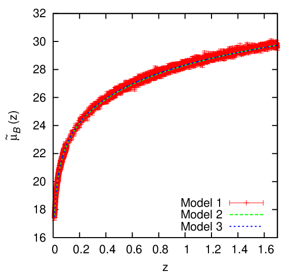
Figure 3 and the upper panels in Figure 2 give a visual impression of the difficulties posed by reconstruction. Figure 3 shows the simulated data for Model 1 with error bars and the exact for Models 2 and 3, which are hardly distinguishable by eye. Figure 2 shows the differences for each dataset with respect to a CDM model with ; models with nontrivial show relatively small deviations from the horizontal line. As we demonstrate below, inverse modeling using Gaussian processes can successfully discriminate between these marginal differences and reconstruct the dark energy equation of state reliably within stated errors.
IV Reconstruction of the Dark Energy Equation of State
As discussed previously, the dark energy equation of state is not directly measurable from the luminosity distance-redshift relation, given in Eqn. (3). The obvious idea of first fitting for and then extracting by taking two derivatives must deal with the noise in the data and the filtering required to estimate the derivatives. Experience with inverse problems has shown that such approaches can easily yield unsatisfactory results. A detailed discussion on the shortcomings of this approach can be found in, e.g., Ref. [46].
A simpler alternative is to assume a hopefully well-motivated parametric form for and then fit for the parameters (for an early discussion about the advantages of this approach, see, e.g., Ref. [46]). For example, if we assume to be constant, the integral over in Eqn. (3) can be solved analytically and the best-fit value for can then be determined from measurements of via, e.g., maximum likelihood techniques. Current data are in good agreement with a constant at the 10% level (for a recent analysis see Ref. [10] and references therein for earlier results). Going beyond this, a weak redshift dependence of may be assumed. One way to realize this is a Taylor expansion of in its redshift evolution, of the form , as suggested in Refs. [22, 23, 24]. However, this parameterization is not well suited for , the regime that holds the most promise to distinguish different models of dark energy [26, 43]. In Ref. [26], the form is suggested as a better alternative (also given previously in Ref. [25]). This parameterization has several nice features: it is well behaved beyond , it has only two parameters and is therefore relatively easy to constrain, and it captures the general behavior of different classes of dynamical dark energy models. The major disadvantage is that the parameterization will only allow reconstruction of monotonic behaviors of . More involved parameterizations have been suggested to address this problem; overviews can be found in Refs. [21, 7]. Although parameter estimation is technically much easier than reconstruction, it can have shortcomings due to poor control over bias [27].
Nonparametric reconstruction methods have received less attention, in part because the current data quality does not fully justify the use of sophisticated inverse methods. Nevertheless, with future data quality in mind, nonparametric techniques can be a powerful alternative for extracting information about . They can capture more complex behavior in and – in principle – can prevent the existence of bias due to a restricted parameterization. Early nonparametric approaches involve a smoothing procedure for either or related quantities at a characteristic smoothing scale, see, e.g. [15, 18].
A somewhat intermediate approach is a piecewise constant description of (see, e.g., Ref. [47]) using basis functions such as top-hat bins or wavelets [20]. In the extreme case of one bin for the whole data range, this method is equivalent to the . parametrization. Determining the optimal number of bins informed by the data is therefore important though not straightforward. Too few bins would erase important information, too many bins would enhance noise to (incorrect) information. In Ref. [16], four redshift bins were used, while Ref. [48] used five redshift bins over a smaller redshift range. In order to obtain uncorrelated estimates of the dark energy parameters in the different bins, a principal component analysis is carried out first. This method has been used recently by the JDEM Figure of Merit Science Working Group [49] to assess the performance of JDEM with respect to constraining the dark energy equation of state. In Ref. [48] a combined analysis of diverse data sets has been performed based on this method and found no evolution in . In contrast to the piecewise constant description of the dark energy equation of state, our approach represents by a continuous Gaussian process, the parameters specifying the process – the so-called hyperparameters – being completely determined as part of the solution of the inverse problem. It is important to distinguish the GP hyperparameters from the parameters of a conventional parametric method. The GP approach is nonparametric, the hyperparameters specifying aspects of the prior distribution in a Bayesian approach (such as properties of the allowed classes of functions). One advantage of this degree of freedom is that one can explicitly use it to test the sensitivity of the posterior distribution to assumptions made about the prior, e.g., the order of differentiability. Here, we make no binning assumptions or assumptions of the discrete properties of the GPs, favorable when working with a physical process that is assumed to be continuous in nature.
In this paper we will study the ansatz and the parameterization suggested in Refs. [25, 26] as reference standards to compare with the GP modeling approach. As a simplification, in the first step of our analysis, we will assume knowledge of the value of and assume perfect calibration, i.e. . In the next step, we will drop these assumptions and include the parameters as part of the estimation process, as would be the case in a more realistic scenario (albeit without directly including non-supernova datasets). To provide a context for the GP approach we will first present an analysis with parameterized models.
IV.1 Parametric Reconstruction


In the study of parametric reconstruction, we follow a Bayesian analysis approach [50]. We focus the analysis on two of the previously discussed models: and and use MCMC algorithms to fit for the model parameters [51], resulting in posterior estimates and probability intervals for , and the parameters that specify the form of . We have consistent priors in all of our models (including the GP model described in the next section) so the results are readily comparable:
| (9) | |||||
| (10) | |||||
| (11) | |||||
| (12) | |||||
| (13) |
and the likelihood
| (14) |
where encapsulates the cosmological parameters to be constrained, i.e., a subset or all of , and . Here the notation “” simply means “distributed according to”. is a uniform prior, with the probability density function for and otherwise. is a Gaussian (or Normal distributed) prior with the probability density function . The squared notation for the second parameter in is used to indicate that is the standard deviation (to prevent possible confusion with the variance ). (The parameters in the distribution do not have this same meaning of mean and standard deviation as in the Normal distribution.) For each case we study, we confirm that the MCMC chains converged by monitoring the trace plots and checking for good mixing and stationarity of the posterior distributions.
The prior for is informed by the 7-year WMAP analysis [52] for a CDM model combining CMB, BAO, and measurement. Since our assumptions on are less strict than we broaden the prior by a factor of two, leading to a Gaussian prior given in Eqn. (11). As discussed earlier, we also allow for an uncertainty in the overall calibration of the supernova data, . We choose a wide, uniform prior for given in Eqn. (12). We consider two cases in all the analyses presented in this paper. In the first case we fix to a fiducial value and reconstruct . This allows us to focus on biases due to assumed parametric forms (parametric models) or possible shortcomings due to the ill-posedness of the inverse problem (GP methodology). In the second case, we let be a free variable within the specified prior, allowing us to study problems with degeneracies that are highlighted when is a nontrivial function of redshift.
IV.1.1 Constant Equation of State
The simplest extension beyond a cosmological constant is to assume that is redshift independent. In this case, Eqn. (5) simplifies to
| (15) | |||||
Current data are in good agreement with this assumption. We will use the ansatz as a first test in attempting to reconstruct all three datasets. As discussed previously, an MCMC algorithm is employed with the chain being run about 10,000 times. Convergence is very quickly attained, within about the first one hundred iterations.
Figure 5 shows the results for the case where we fix and assume perfect calibration. As expected, the reconstruction works extremely well for the model where in fact (left panel). The best fit value for and its probability intervals (PIs) are given in Table 1 and match the chosen value within small errors. Not surprisingly, the results for the models with time varying are rather inaccurate. For dataset 2, the value for is predicted slightly higher than the average would be. In general, a larger leads to a lower . As can be seen in Figure 2, is slightly below the CDM model for this dataset. The one-parameter best fit for therefore has to be high in order to capture this behavior, if we do not allow any other parameter to vary. For the third dataset, we find a similar situation. As can be seen in Figure 2 in the right panel, is below the fiducial model. Capturing this behavior with only one parameter to vary, , leads to a value in order to fit the behavior in reasonably well.
| Set | ||||
|---|---|---|---|---|
| 1 | 0.27 | 0 | ||
| 2 | 0.27 | 0 | ||
| 3 | 0.27 | 0 | ||
| 1 | ||||
| 2 | ||||
| 3 |


In the next step, we allow and to vary within the assumed priors given in Eqs. (11) and (12). The results for (including the truth) are shown in Figure 5. The best fit values including error bars are given in Table 1. Since and are highly correlated they must be sampled jointly with a covariance structure obtained after running the process for some time. As in the case of and fixed, the analysis is robust and works well for the case of Although the error bands increase, the best fit values for all three parameters are very close to the assumed model values. In the two cases of variable , the strong degeneracy between and becomes very apparent, as both and influence the behavior of in a very similar way: This bias on will disappear if other datasets such as CMB data are included to provide good constraints on . For the second dataset, where has a downward trend for higher , the behavior can be captured by a low value for and a high value for , or vice-versa. The best fit values will also account for the curvature in and we find that the best-fit model underpredicts and overpredicts . This degeneracy can only be broken if we have better estimates for . For dataset 3 the situation is even more severe: in order to capture the slope of , the estimates for both parameters, and , are off, is highly overestimated, while the value for is underestimated and in fact does not even go through the true any more as can be seen in Figure 5. This example demonstrates the bias that can be introduced in the reconstruction of if the assumed form for is too restricted and degeneracies are present. Also note that the true result no longer falls within the predicted error bands.
For both datasets, the prediction for , which is mainly anchored by the amplitude of the measurements for , is close to the true value. We also note that the “truth” for and is not exact since we are working with one finite realization for each dataset.
IV.1.2 Parameterization


We now turn to the investigation of a commonly used parameterization of the dark energy equation of state given by Refs. [25, 26]:
| (16) |
As for the case , one integral in Eqn. (3) can be solved analytically and the expression for simplifies to:
This parameterization allows for a weak monotonic time dependence in and should therefore capture the behavior of our second model reasonably well.
Following the analysis in the previous case (), we first fix and to their fiducial values. The results are summarized in Figure 6 and Table 2. For the dataset the parameterization picks up a very small variation in but the prediction is well within errors. The mild variation with in the second dataset is captured reasonably well. A rather high value for leads to a pull-down of . This is then compensated by a large positive value for which leads to an upturn in .
For the third dataset the parameterization is not quite flexible enough. While the overall behavior (the rise at high redshift) is captured, the S-shape of the underlying equation of state cannot be extracted. Moreover, in an attempt to fit the data, the value of equation of state today is decreased to . This decrease leads to an upturn of while the large negative value for acts in the opposite direction. The parameterization finds a time dependence in , but not of the correct specific form as would be required for distinguishing different models of dark energy.
The results including estimations for and are similar. As for the parameterization, the parameters are all sampled jointly because of their strong correlations. These correlations degrade the accuracy of the reconstruction. For the first dataset, the prediction for is slightly high which in turn amplifies a time dependence in the best fit for which does not exist in the original dataset. Again, the error bars are large and clearly is well within the error bounds. For the second data set, the prediction for is rather accurate. For dataset 3, is overpredicted which leads to a slight degradation in the prediction for itself. The values for and are similar to the case of fixed .
| Set | ||||
| 1 | 0.27 | 0 | ||
| 2 | 0.27 | 0 | ||
| 3 | 0.27 | 0 | ||
| 1 | ||||
| 2 | ||||
| 3 | ||||
| Set | ||||
| 1 | ||||
| 2 | ||||
| 3 | ||||
| 1 | ||||
| 2 | ||||
| 3 |
Overall, the parameterization provides a reasonable description of the data, especially for moderately varying , as is expected. The drawback is obvious: rapid changes in as shown in dataset 3 cannot be captured.
IV.2 Nonparametric Reconstruction: Gaussian Process Model
The previous exploration of the standard parametric methods makes it clear that as long as the data correspond to the models that the methods are designed for (e.g., if is in fact constant, the ansatz will obviously lead to the best result), the results are rather good. However, as soon as datasets are introduced for which the parameterizations are not flexible enough to track the true behavior of , the analysis is susceptible to unacceptable levels of bias in determining modeling and cosmological parameters.
It is common practice to employ a parametric form for and then assess the robustness of the result by a goodness of fit test. For example, Ref. [28] uses a Bayesian information criterion (BIC) statistic for this task. We applied the BIC model comparison criteria for the two parametric reconstruction approaches without much success – instead of choosing the model that corresponds to the truth (which in case of dataset 2 and 3 is the parametrization over ) the BIC always preferred the parametric form with the least parameters, in this case
A nonparametric form of can address some of the shortcomings of parametric reconstruction methods. We now describe a new, nonparametric method based on GP modeling [31, 32]. As mentioned previously, a GP is a stochastic process, which in our case is indexed by . The defining property of a GP is that the vector that corresponds to the process at any finite collection of points follows a multivariate normal (MVN) distribution. Gaussian processes are elements of an infinite dimensional space, this is the sense in which they provide a nonparametric method for curve fitting. They are characterized by a mean and a covariance function, often defined by a small number of hyperparameters.
We assume that the data errors are Gaussian and use the same likelihood as in the treatment of the parameterized models. The use of Bayesian estimation methods (including the MCMC algorithm) allows us to estimate the hyperparameters of the GP correlation function together with any other parameters, comprehensively propagating all estimation uncertainties [51]. Using the definition of a GP, we assume that, for any collection , follow a multivariate Gaussian distribution with a constant negative mean and exponential covariance function written as
| (18) |
Here is a free parameter that, together with and the parameters defining the likelihood, are fit from the data. The form of the assumed correlation function implies that, theoretically, there is non-zero correlation between any two points. controls the exponential decay of the correlation as a function of distance in redshift, but it does not provide a bound for the correlation between two points. This is analogous to the concept of standard deviation – many, but not all, of the observations are within one standard deviation of the mean, and most are within two, but there is no theoretical bound that all observations have to fall within. In principle, we could include an explicit noise term in the correlation (a so-called “nugget”). Instead, we chose to include the noise term in the likelihood equation (14) from which it will propagate to the GP.
The value of influences the smoothness of the GP realizations: for , the realizations are smooth with infinitely many derivatives, while leads to rougher realizations suited to modeling continuous non-differentiable functions. Here we use to allow for maximum flexibility in reconstructing . (For a comprehensive discussion of different choices for covariance functions and their properties, see Ref. [32].) The mean of the GP is taken to be fixed. has a prior of and has a prior of . is an inverse Gamma distribution prior, with the probability density function , with . The probability distribution of the prior is given by . Figure 8 shows an example of the priors for and the two GP model parameters and for dataset 1. The posteriors indicate that the data are informative about and reasonably informative about . As for the parametric reconstruction, is given a prior based on currently available estimates.


We set up the following GP for :
| (19) |
Choosing a mean value of -1 is natural, given current observational constraints on . Even though the mean is fixed, each GP realization will actually have a different mean with a spread controlled by . For the second and third dataset we adjusted the means during the analysis to slightly different values suggested by preliminary runs. This adjustment is purely informed by the data and demonstrates the flexibility of the approach. In principle, the mean could also be left as a free parameter. After the adjustment we measured the posterior mean and ensured that it was close to the prior mean. Table 3 summarizes the prior and posterior means for the final analysis.
| Set | Prior Mean | Posterior Mean |
|---|---|---|
| 1 (, ) fixed | -1.00 | -1.01 |
| 1 (, ) free | -1.00 | -1.02 |
| 2 (, ) fixed | -0.94 | -0.90 |
| 2 (, ) free | -0.87 | -0.88 |
| 3 (, ) fixed | -0.7 | -0.71 |
| 3 (, ) free | -1.00 | -1.04 |
Next, recall that we have to integrate over (Eqn. 3):
| (20) |
We use the fact that the integral of a GP is also a GP with mean and correlation dependent on the original GP [31]. Therefore results in a second GP defined as:
| (21) |
where we choose . The mean value for this GP is simply obtained by integrating Eqn. (20) for the mean value of the GP for . We can now construct a joint GP for and :
| (22) |
with
| (23) | |||||
| (24) | |||||
| (25) |
The mean for given can be found through the following relation:
| (26) |
Note that we never have to calculate the double integral in which would be numerically expensive. More details about each step in the GP model algorithm are given in Appendix A.
| Set | |||||
|---|---|---|---|---|---|
| 1 | 0.27 | 0 | |||
| 2 | 0.27 | 0 | |||
| 3 | 0.27 | 0 | |||
| 1 | |||||
| 2 | |||||
| 3 |
Following our practice for the parameterized reconstruction methods, we first apply the GP-based technique fixing the values for and . The results are shown in Figure 10. Reconstruction from the GP model for is remarkably accurate for all three data sets. (The noise in the predictions is due to the choice of the functional form of the covariance function.) In particular, the reconstruction for the third dataset, where the parameterized model did not fare well, is very good. Table 4 gives the results for the GP model hyperparameters and for all three models. Larger values for indicate a smoother reconstructed function. For a model with more variation in the data and crossing the mean several times, the correlation length would be smaller than for the models investigated here. Our analysis shows that the is the smallest for the dataset that varies the most (dataset 3), as expected. Since even the third dataset is not varying strongly, is still close to one (note that is not allowed). In addition, the interplay between and which determine the overall covariance function is non-trivial – the simultaneous fitting of and is therefore an important aspect of our approach.
Last, we study the results from the GP model, letting and vary. The results are shown in Figure 10. As for the two parameterized models, degeneracies degrade the results in the cases of varying . For the case of the prediction for is very close to the input value (see Table 4 for the best-fit values for and and the GP model parameters), and the reconstruction for , albeit somewhat noisy, is very close to the truth. For the second model, the best-fit value for is slightly low, but correct within the error bars. The reconstruction is also in this case very accurate. For the third dataset the best fit value for is above the true value, leading to a lower result for . The GP model approach captures the overall behavior of the true within the error bands. However, the problem due to the degeneracy between and becomes very apparent in this case. The GP model approach finds a solution that overestimates with a rather flat . As we show in the next section, this is a good fit to the data but does not give a particular good match to the true . These results will certainly improve if we have stronger constraints on from different datasets, e.g., CMB or baryon acoustic oscillation measurements to break the degeneracies between and .
IV.3 Comparison of the Different Approaches
In order to summarize our findings, we now provide a brief comparison of the parametric and nonparametric reconstruction results. We consider two metrics for this comparison: (i) the accuracy of the reconstructed form of given that the exact answer is known, and (ii) the accuracy with which the predicted fits the data. As mentioned before, more involved statistical techniques such as BIC did not lead to satisfying results, as the simplest parametrization was always identified as the best – which is obviously not the case for datasets 2 and 3.
| Dataset 1 | Dataset 2 | Dataset 3 | |
|---|---|---|---|
| (, fixed) | 0.00001 | 0.0044 | 0.1000 |
| (, free) | 0.00004 | 0.0058 | 0.3050 |
| (, fixed) | 0.00003 | 0.0001 | 0.0034 |
| (, free) | 0.0175 | 0.0019 | 0.0109 |
| GP (, fixed) | 0.0006 | 0.0003 | 0.0014 |
| GP (, free) | 0.0006 | 0.0012 | 0.1439 |


Table 5 shows a simple measure of how well the exact functional form of has been captured by the three different approaches. We calculate the mean square error of the reconstructed history for with respect to the perfect input as shown in the lower panels of Fig. 2 – the smaller the error the better the reconstruction result. This simple test has two minor shortcomings – first, it does not account for the realization noise in the history of underlying the simulated data so the error will never be zero. In order to obtain the true we would have to perform two derivatives of the noisy simulated data which would render this test basically meaningless. Second, the error bands of the predictions are not taken into account. Nevertheless, this comparison should provide some information about how well the different methods perform compared to each other.
For the first dataset . the parametric reconstruction ansatz provides – not surprisingly – the best results; the history for is captured extremely well as is with small errors. For dataset 1, the GP model provides a more accurate answer than the parameterization in the case of free. This is mainly due to the fact that once the parameterized form has picked up some curvature in , the reconstructed will depart more and more from at higher . The GP model however is flexible enough to avoid such a behavior and stays close to over the whole redshift range. For dataset 2, the GP model performs slightly better than the two parametric reconstruction approaches for similar reasons as for dataset 1. The parametrization picks up some time-dependence in the low- regime which overestimates the curvature of at higher while the GP approach reconstructs reasonably well over the whole redshift range and therefore has a smaller mean square error. For the third dataset, the mean square error for the GP model is smallest in the case of fixed but for free kept it is worse than the result from the parametrization. For this last case (dataset 3 and and free) we employ another assessment of the accuracy of the prediction which highlights the well-known degeneracy between and . We only consider the parametrization and the GP model approach for this test, since the parametrization has obvious shortcomings in this case.
For each case we fit the result and then we find the associated fit for . Then we determine the difference between the predicted and the input for our simulated data. We show the residuals in Figure 11. The left figure shows the residuals for the parametrization, the right figure for the GP reconstruction. The solution for found with the GP model is clearly a good fit to the data – it performs slightly better than the parametrized form in the low redshift range. Due to the the degeneracy between and the overall reconstruction of is on the other hand worse for the GP model – this result will improve with tighter constraints on and complementary datasets such as BAO measurements which help to break the degeneracy.
V Conclusions
Characterizing the behavior of the dark energy equation of state is a first step in understanding the nature and origin of dark energy. Although a simple cosmological constant model is consistent with current observations, the implied numerical value has no theoretical explanation. Alternative dynamical models of dark energy generically predict time variations in and a robust detection of such a time dependence is one of the first targets in dark energy studies. Supernova measurements remain a very promising probe of and future sky surveys can in principle measure with high accuracy.
In order to fully exploit the power of future measurements, a reliable and robust reconstruction method is required. In this paper we have introduced a new reconstruction approach based on GP modeling. The approach is nonparametric with modeling hyperparameters constrained directly from the data. We have demonstrated that we can extract nontrivial behavior of as a function of redshift with data of the quality expected from future surveys. We have contrasted our new method against two approaches, an assumed cosmological constant, and one with a simple two-parameter model of the variation of . Both of these models are effective descriptions for only a limited class of possible behaviors of . In contrast, the generality of the GP approach results in accurate reconstruction of potentially complex variability in .
The GP model approach makes only mild smoothness assumptions about which are reasonable if we expect that the accelerated expansion of the Universe is due to a physically well motivated reason. The major ingredient for the GP model is specified by the covariance function . While the choice of the specific form for is up to the modeler, the GP approach is rather robust to this choice and the major hyperparameters influencing are informed by the data themselves. In addition to choosing a covariance function, we have to specify a set of priors for cosmological and model parameters. These priors have to be broad enough to include the truth but should not be so broad that the Bayesian approach does not converge. Both model and cosmological parameters are then jointly determined from the data. While the Bayesian approach is computationaly rather intensive, it has the great advantage that it provides robust error bands. The approach outlined here for the analysis of supernova measurements can easily be extended to include different cosmological probes such as data from CMB and BAO observations; work in this direction is currently in progress. Moreover, the GP-based MCMC procedure can be integrated within supernova analysis frameworks, e.g., SNANA [53] as a cosmology fitter, following the general methodology presented in Ref. [34].
Appendix A GP model algorithm
In this appendix we provide implementation details of the GP algorithm used to reconstruct . The GP model approach requires the estimation of several variables: the correlation hyperparameters ( and ), the Gaussian process points [ with , or rather with , the variance parameter (), along with the physical parameters of interest ( and ). and can be added as extra steps; for simplicity we do not include them in the discussion here (we did include them in our analysis presented in the main body of the paper.)
A Gaussian process is defined by its mean and correlation function. We set the prior mean of the Gaussian process to for stability; other values are found to be equally acceptable when the true mean of is near . Even though the mean is fixed, the posterior mean will not be exactly but will have a distribution spread around . In the case when the true mean is not the posterior value of the mean of will indicate this. Preliminary exploration of the posterior of can then be used to set the prior mean for subsequent runs, which provides more stable results.
In the correlation function, the parameter should be set as a constant beforehand in the range of 1 to 1.9999, setting it exactly equal to 2 can cause numerical instability in the covariance matrix, and values above 2 are not mathematically valid values for the process. The parameter controls the smoothness of the overall GP: will produce a flexible continuous GP but it will not be differentiable anywhere, while produces a much smoother continuous GP that is infinitely differentiable everywhere. In order to allow for maximum flexibility we choose throughout the paper. The correlation length is a free parameter in the GP model and its value is informed by the data. It is highly correlated to and which makes the interpretation of its final value not straightforward. It is strictly limited to the region of [0,1) and the GP is not defined for the limiting case of . After investigation we found that has a much smaller role in the determination of the nature of the GP in comparison to and .
Integration of the Gaussian process requires a grid for numerical integration. Let be the number of supernova data points in our dataset, and be a finite number of Gaussian process points over this region for evaluation. During the integration we add partition points between each GP point. Our resulting integrated process has points. This provides a dense enough grid to carry out an accurate numerical integration for the outer integral without slowing down the computations. We find that an around 50 to 100 is sufficient, and an between 3 and 5 is a good balance between accuracy and speed.
As with the parametric models, we employ Bayesian methods where we use our priors and likelihood to obtain a posterior that can then be sampled with an MCMC algorithm. In our case, with our given likelihood function (given in Eqn. (14)), this leads to the following posterior for the parameters of interest:
| (27) |
here denotes an arbitrary GP with parameters and . is the unknown variance parameter from the likelihood equation and , , and are “observed” values from the simulated dataset.
Instead of the usual Gaussian process formulation shown in Eqn. (27), we choose an altered form to allow for slower changes in the GP and a more localized search. We let and . This leads to the following posterior:
| (28) |
In this setup, we propose a GP and transform it to . We then keep track of and make our next proposal based on these values and not on the . Thus we are allowing the proposal to make finer changes each time to boost the acceptance rate, which tends to be problematic if we were to propose directly.
The explicit procedure for estimating the process parameters is as follows and employs standard MCMC techniques.
- 1.
Initialize all variables: , , and . will be a vector with points in our GP and has points. We run this algorithm times. Set all tuning parameters, , which need to be tuned until good mixing occurs.
- 2.
Propose
- (a)
Compute the covariance matrix
- (b)
Compute the Cholesky decomposition for
- (c)
Compute the special with Chebyshev-Gauss quadrature.
- (d)
We want where
- (e)
where the definite integrations in are done numerically through summations of the trapezoid algorithm.
- (f)
Accept the proposal with probability let , otherwise .
- (a)
- 3.
Draw
- (a)
Compute
- (b)
where the definite integrations in are done numerically through summations of the trapezoid algorithm.
- (c)
Accept with probability .
- (a)
- 4.
We propose a non-standard for the GP. We start by drawing a proposal for , where is the identity matrix.
- (a)
Compute
- (b)
- (c)
Accept with probability letting and the corresponding GP realization is
- (a)
- 5.
- 6.
Repeat steps 2-6, times and rerun the entire algorithm as needed after resetting the tuning parameters
Acknowledgements.
The authors acknowledge support from the LANL Institute for Scalable Scientific Data Management. Part of this research was supported by the DOE under contract W-7405-ENG-36. UA, SH, KH, and DH acknowledge support from the LDRD program at Los Alamos National Laboratory. KH was supported in part by NASA. SH and KH acknowledge the hospitality of the Aspen Center for Physics, where part of this work was carried out. We are indebted to Andreas Albrecht, Eric Linder, Adrian Pope, Martin White, and Michael Wood-Vasey for several useful discussions.References
- [1] S. Perlmutter et al. [Supernova Cosmology Project Collaboration], Astrophys. J. 517, 565 (1999) [arXiv:astro-ph/9812133].
- [2] A.G. Riess et al. [Supernova Search Team Collaboration], Astron. J. 116, 1009 (1998) [arXiv:astro-ph/9805201].
- [3] D. Schlegel, M. White, and D. Eisenstein, arXiv:0902.4680 [astro-ph.CO]
- [4] https://www.darkenergysurvey.org/
- [5] http://jdem.gsfc.nasa.gov/
- [6] http://www.lsst.org/lsst
- [7] J. Frieman, M. Turner and D. Huterer, Ann. Rev. Astron. Astrophys. 46, 385 (2008) [arXiv:0803.0982 [astro-ph]].
- [8] M.S. Turner and M.J. White, Phys. Rev. D 56, 4439 (1997) [arXiv:astro-ph/9701138].
- [9] C. Wetterich, Nucl. Phys. B 302, 668 (1988); B. Ratra and P.J.E. Peebles, Phys. Rev. D 37, 3406 (1988); P.J E. Peebles and B. Ratra, Astrophys. J. 325, L17 (1988); R. R. Caldwell, R. Dave and P. J. Steinhardt, Phys. Rev. Lett. 80, 1582 (1998) .
- [10] M. Hicken et al., Astrophys. J. 700, 1097 (2009) [arXiv:0901.4804 [astro-ph.CO]].
- [11] R. Amanullah et al., Astrophys. J. 716, 712 (2010) [arXiv:1004.1711 [astro-ph.CO]].
- [12] D. Huterer and M.S. Turner, Phys. Rev. D 60, 081301 (1999)
- [13] A.A. Starobinsky, JETP Lett. 68, 757 (1998) [Pisma Zh. Eksp. Teor. Fiz. 68, 721 (1998)] [arXiv:astro-ph/9810431].
- [14] Y. Wang and P. Mukherjee, Astrophys. J. 606, 654 (2004) [arXiv:astro-ph/0312192].
- [15] R.A. Daly and S.G. Djorgovski, Astrophys. J. 597, 9 (2003) [arXiv:astro-ph/0305197].
- [16] D. Huterer and A. Cooray, Phys. Rev. D 71, 023506 (2005) [arXiv:astro-ph/0404062].
- [17] B.F. Gerke and G. Efstathiou, Mon. Not. Roy. Astron. Soc. 335, 33 (2002) [arXiv:astro-ph/0201336].
- [18] A. Shafieloo, U. Alam, V. Sahni and A.A. Starobinsky, Mon. Not. Roy. Astron. Soc. 366, 1081 (2006).
- [19] C. Zunckel and R. Trotta, Mon. Not. Roy. Astron. Soc. 380, 865 (2007) [arXiv:astro-ph/0702695].
- [20] A. Hojjati, L. Pogosian, and G.-B. Zhao, arXiv:0912.4843 [astro-ph.CO].
- [21] V. Sahni and A.A. Starobinsky, Int. J. Mod. Phys. D 15, 2105 (2006) [arXiv:astro-ph/0610026].
- [22] A.R. Cooray and D. Huterer, Astrophys. J. 513, L95 (1999) [arXiv:astro-ph/9901097].
- [23] I. Maor, R. Brustein and P.J. Steinhardt, Phys. Rev. Lett. 86, 6 (2001) [Erratum-ibid. 87, 049901 (2001)] [arXiv:astro-ph/0007297].
- [24] J. Weller and A.J. Albrecht, Phys. Rev. Lett. 86, 1939 (2001) [arXiv:astro-ph/0008314].
- [25] M. Chevallier and D. Polarski, Int. J. Mod. Phys. D 10, 213 (2001) [arXiv:gr-qc/0009008].
- [26] E.V. Linder, Phys. Rev. Lett. 90, 091301 (2003) [arXiv:astro-ph/0208512].
- [27] F. Simpson and S.L. Bridle, Phys. Rev. D 73, 083001 (2006), arXiv:astro-ph/0602213.
- [28] C. Genovese, P. Freeman, L. Wasserman, R. Nichol, and C. Miller, Ann. Appl. Stat. 3, 144 (2009) [arXiv:0805.4136 [astro-ph]].
- [29] M.J. Mortonson, W. Hu and D. Huterer, Phys. Rev. D 79, 023004 (2009) [arXiv:0810.1744 [astro-ph]].
- [30] T. Holsclaw, et al. (in preparation).
- [31] S. Banerjee, B.P. Carlin, and A.E. Gelfand, Hierarchical Modeling and Analysis for Spatial Data, New York: Chapman and Hall (2004).
- [32] C.E. Rasmussen and K.I. Williams, Gaussian Processes for Machine Learning (MIT Press, 2006); http://www.gaussianprocess.org/gpml/
- [33] K. Heitmann, D. Higdon, C. Nakhleh and S. Habib, Astrophys. J. 646, L1 (2006) [arXiv:astro-ph/0606154].
- [34] S. Habib, K. Heitmann, D. Higdon, C. Nakhleh and B. Williams, Phys. Rev. D 76, 083503 (2007) [arXiv:astro-ph/0702348].
- [35] K. Heitmann, D. Higdon, M. White, S. Habib, B.J. Williams and C. Wagner, Astrophys. J. 705, 156 (2009) [arXiv:0902.0429 [astro-ph.CO]].
- [36] E. Lawrence, K. Heitmann, M. White, D. Higdon, C. Wagner, S. Habib and B.J. Williams, Astrophys. J. 713, 1322 (2010) [arXiv:0912.4490 [astro-ph.CO]].
- [37] B.J. Brewer and D. Stello, Mon. Not. Roy. Astron. Soc. 395, 226 (2009) [arXiv:0902.3907].
- [38] M.J. Way, L.V. Foster, P.R. Gazis and A.N. Srivastava, Astrophys. J. 706, 623 (2009) [arXiv:0905.4081 [astro-ph.IM]].
- [39] D.G. Bonfield, Y. Sun, N. Davey, M.J. Jarvis, F.B. Abdalla, M. Banerji and R.G. Adams, Mon. Not. Roy. Astron. Soc. 405, 987 (2010) [arXiv:0910.4393 [astro-ph.IM]].
- [40] U. Alam, V. Sahni and A.A. Starobinsky, JCAP 0702, 011 (2007) [arXiv:astro-ph/0612381].
- [41] E. Komatsu et al., Astrophys. J. Supp. 180, 330 (2009) [arXiv:0803.0547 [astro-ph]].
- [42] R. Kessler et al, Astrophys. J. Suppl. 185, 32 (2009) [arXiv:0908.4274 [astro-ph.CO]].
- [43] E.V. Linder and D. Huterer, Phys. Rev. D 67, 081303 (2003).
- [44] G. Aldering et al. [SNAP Collaboration], arXiv:astro-ph/0405232.
- [45] P.S. Corasaniti, B.A. Bassett, C. Ungarelli and E.J. Copeland, Phys. Rev. Lett. 90, 091303 (2003) [arXiv:astro-ph/0210209].
- [46] J. Weller and A. Albrecht, Phys. Rev. D 65, 103512 (2002) [arXiv:astro-ph/0106079].
- [47] D. Huterer and G. Starkman, Phys. Rev. Lett. 90, 031301 (2003) [arXiv:astro-ph/0207517].
- [48] P. Serra, A. Cooray, D. E. Holz, A. Melchiorri, S. Pandolfi and D. Sarkar, Phys. Rev. D 80, 121302 (2009) [arXiv:0908.3186 [astro-ph.CO]].
- [49] A.J. Albrecht et al., arXiv:0901.0721 [astro-ph.IM].
- [50] A. Gelman, B. Carlin, H. Stern, and D. Rubin, Bayesian Data Analysis, New York: Chapman and Hall (2004).
- [51] D. Gamerman and H.F. Lopes, Markov Chain Monte Carlo: Stochastic Simulation for Bayesian Inference, New York: Chapman and Hall (2006).
- [52] E. Komatsu et al., arXiv:1001.4538 [astro-ph.CO].
- [53] R. Kessler et al. Publ. Astron. Soc. Pac. 121, 1028 (2009), arXiv:0908.4280 [astro-ph.CO].