An approximative calculation of the fractal structure in self-similar tilings
Abstract
Fractal structures emerge from statistical and hierarchical processes in urban development or network evolution. In a class of efficient and robust geographical networks, we derive the size distribution of layered areas, and estimate the fractal dimension by using the distribution without huge computations. This method can be applied to self-similar tilings based on a stochastic process.
Keywords:
Complex Network Science, Geographical Network, Random Fractal, Markov Chain, Urban Planningpacs
89.75.Fb, 02.50.Ga, 02.70.-c, 89.20.Ff, 89.40.-aI Introduction
Fractal nature is observed in our real-life infrastructures of urban spatial organization and many technological networks. Indeed, the fractal dimensions of land-use and area-perimeter have been measured in real data of urban cities [1][2]. Similar structures with mixing of dense and sparse areas of nodes have been found in router networks [3], air transportation networks [4], and mobile communication networks [5]. These studies show that the spatial distribution of human activities is inhomogeneous and concerning with the population density. Thus, there commonly exists a hierarchical structure based on statistical self-similarity beyond regular mathematical models such as Sierpinski gasket and carpet. In other words, fractal behavior is not limited to objects with a regular morphology, but can be introduced by iterative evolutionary processes of subdivision or growing at different levels of scaling.
Recently, a multi-scale quartered (MSQ) network, which is stochastically constructed by a self-similar tiling, has been proposed [6][7]. The geographical network embedded on a planar space has several advantages [6]: the robustness of connectivity against failures and attacks, the bounded short path lengths, and the decentralized routing algorithm [8] in a distributed manner. Furthermore [7], it is more efficient (economic) with shorter link lengths and more suitable (tolerant) with lower load for avoiding traffic congestion than the state-of-the-art geometric growing networks [9, 13, 14, 15, 10, 11, 12] and the spatially preferential attachment models with various topologies ranging from river to scale-free geographical networks. These properties are useful for the future self-organized design of wide-area wireless ad hoc networks.
This paper investigates the size distribution of faces iteratively divided in the generation process of a MSQ network. In particular, we derive an approximative equation for the averaging behavior of random process, and apply it to easily estimate the fractal dimension of such a self-similar tiling.
II MSQ network
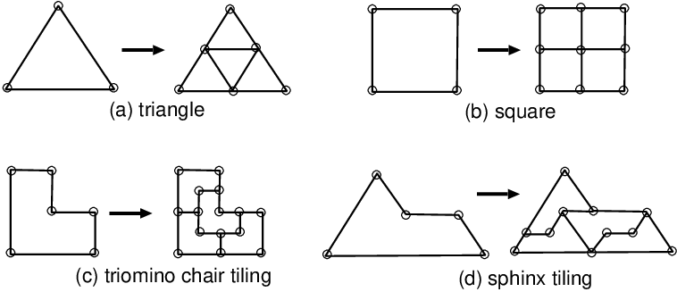
For generating a MSQ network, the following process is repeated from an initial tiling which consists of same shaped faces. At each time step, a face is chosen, e.g., with a probability proportional to the population in the space of a face for the load balancing of communication requests, or uniformly at random. Then, as shown in Fig. 1, four smaller faces are created in the chosen face, and a planar network is self-organized on a geographical space. Such a fractal structure is also observed in urban road networks [16] [17]. Note that the MSQ network includes a Sierpinski gasket obtained by a special selection when each triangle, except the central one, is hierarchically divided, however its fractal dimension differs to that in the average behavior of the following random selection.
III Infinite state Markov chain
For simplicity, we treat the uniformly random selection of a face, whose case corresponds to general positions of nodes in the geographical network. In addition, even if a face in the area of high population density tend to be chosen for the subdivision, the assigned population to a node in its territory is asymptotically balanced, then the behavior closes to the case of random selections in course of time. In this setting, the subdivision process makes an infinite state Markov chain as illustrated in Fig. 2. Here, we consider a vector as the state of Markov chain, whose element represents the number of faces at time step on the layer defined by decreasing order of size. A face on the layer is chosen with the probability at the next step , then the sate is changed from to , where denotes the total number of faces at , and is the initial number. Note that is time-dependent on a selected path for the decision tree from the top to the bottom in Fig. 2, equivalently on a selection sequence of faces. Thus, the above Markov chain is different from the Galton-Watson type branching process with a time-independent probability for generating offsprings [18].

We obtain the averaging behavior for
| (1) |
This can be written as
| (2) |
since a face on the layer chosen with the probability is divided into four smaller ones which belong to the layer , therefore a face on the layer contributes to increase the number of faces on the layer . For a large , by noticing and substituting into the right-hand side of Eq. (1), it is
Using because of , Eq. (2) is rewritten to
| (3) |
We numerically confirm that the average behavior of the Markov chain is well fitting to the solution for Eq. (3) as shown in Fig. 3. Here, the cross, asterisk, open square, and closed square marks correspond to the average of 100 states reached at each time , and , respectively, on the decision tree from the initial state in Fig. 2. The four types of dashed curves correspond to the distributions calculated by Eq. (3) until these times. The solid curve fitting with the closed square marks is the approximation by a normal distribution. Note that the averaged or calculated number of faces on each layer at is normalized as the relative frequency . This bell-shaped distribution means that there exist a mixing of dense and sparse areas with various sizes of faces whose majorities have the intermediate sizes. Figure 4 shows the mean and the variance of the distribution . The upper and lower triangle marks denote the mean and the variance of the distribution obtained for the Markov chain. The solid and dashed lines denote the corresponding results for Eq. (3). In Fig. 5, the circle marks and dotted piecewise linear line denote the skewness of these distributions for the Markov chain and for Eq. (3), respectively. The mean and the variance grow as , while the skewness is almost constant around 0.2. Although the is asymptotically a Poisson distribution with a same value for the mean and the variance as mentioned in the Appendix, it is rather fitting with the approximation by Eq. (3) in a finite size.


On the basis of the numerically obtained , the fractal dimension is estimated as 1.2 (a similar value is obtained for a chair or a sphinx tilling [19]) by using a cover-based method in the hierarchically coarse measure of doubling link length on each layer until . Figure 6 shows an example at the state . The number of covered areas (gray rectangles) is
where we set the number of initial coverings for a square tiling. It depends on the primitive shape; for a triangle tiling, and for a chair or a sphinx tiling. In general for a large , we calculate from
| (4) |
the total number of faces in the completely recursive division , the number of holes without subdivisions , and . Three terms in the right-hand side of Eq. (4) correspond to thick, thin solid lines, and dashed lines in Fig. 6. Since there is one-to-one correspondence between the divided four faces and the cross-edges in a square at each layer , e.g., by applying a clockwise mapping rule, represents this effect on the covering. However, the 2nd and 3rd terms are replaced by for a triangle tiling, and by for a chair or a sphinx tiling. We emphasis that our method can be performed by only using the calculated without both averaging and image processings in a box-counting method.

We should remark that the continuous approximation with respect to time and space variables for both sides of Eq. (3)
gives an incorrect solution, which keeps the shape in the traveling wave
where a function is determined by the initial distribution, and .
IV Conclusion
Considering the stochastic network construction [6][7] as a Markov chain, the size distribution of the divided faces has been investigated. We have shown, by numerically solving Eq. (3) as the average behavior, that the mean and the variance are proportional to , while the skewness is small positive. In a realistic finite size , this approximation of is fitting better than the asymptotical Poisson solution for the interactive particle system (see the Appendix). From the distribution , the fractal dimension is estimated as without huge computations of averaging and image processings in the conventional box-counting method. The proposed method can be applied to other self-similar tilings based on a stochastic process. Furthermore, it would be interesting to discuss a self-similar modeling which reproduces the fractal structures of urban road [16][17], air-sea transportation [4], communication [5] networks.
Acknowledgements.
The author would like to thank Prof. Norio Konno in Yokohama National University for suggesting the theoretical analysis in the Appendix. This research is supported in part by a Grant-in-Aid for Scientific Research in Japan, No. 21500072.References
- [1] M. Batty, and P.A. Longley Fractal Cities: A Geometry of Form and Function, Academic Press, London, 1994.
- [2] P. Franlhauser, “The Fractal Approach: A new tool for the spatial analysis of urban agglomerations,” Population: An English Selection , Vol. 10, pp. 205-240, 1998.
- [3] S.-H. Yook, H. Jeong, and A.-L. Barabási, “Modeling the Internet’s large-scale topology,” PNAS Vol. 99, No. 21, pp. 13382-13386, 2002.
- [4] R. Guimerà, S. Mossa, A. Turtschi, and L.A.N. Amaral, “The worldwide air transportation network: Anomalous centrality, community structure, and cites’ global roles,” PNAS Vol. 102, No. 22, pp. 7794-7799, 2005.
- [5] R. Lambiotte, V.D. Blondel, C. de Kerchove, E. Huens, C. Prieur, Z. Smoreda, and P.V. Dooren, “Geographical dispersal of mobile communication networks,” Physica A Vol. 387, pp. 5317-5325, 2008.
- [6] Y. Hayashi, “Evolutionary construction of geographical networks with nearly optimal robustness and efficient routing properties,” Physica A Vol. 388, pp. 991-998, 2009.
- [7] Y. Hayashi, and Y. Ono, “Geographical networks stochastically constructed by a self-similar tiling according to population,” Phys. Rev. E Vol. 82, pp. 016108-1-9, 2010.
- [8] P. Bose, and P. Morin, “Competitive Online Routing in Geometric Graphs,” Theoretical Computer Science Vol. 324, No. 2-3, pp. 273-288, 2004.
- [9] Z. Zhang, S. Zhou, Z. Su, T. Zou, and J. Guan, “Random Siepinski network with scale-free small-world and modular structure,” Euro. Phys. J. B Vol. 65, pp. 141-147, 2008.
- [10] T. Zhou, G. Yan, and B.-H. Wang, “Maximal planar networks with large clustering coefficient and power-law degree distribution,” Phys. Rev. E Vol. 71, pp. 046141-1-11, 2005.
- [11] Z. Zhang, and L. Rong, “High dimensional random Apollonian networks,” Physica A Vol. 364, pp. 610-618, 2006.
- [12] J.P.K. Doye, and C.P. Massen, “Self-similar disk packings as model spatial scale-free networks,” Phys. Rev. E, Vol. 71, pp. 016128-1-11, 2005.
- [13] L. Wang, F.Du, H.P. Dai, and Y.X. Sun, “Random pseudofractal scale-free networks with small-world effect,” Eur. Phys. J. B Vol. 53, pp. 361-366, 2006.
- [14] H. D Rozenfeld, S. Havlin, and D. ben-Avraham, “Fractal and transfractal recursive scale-free nets,” New J. of Phys. Vol. 6, pp. 175-1-15, 2006.
- [15] S.N. Dorogovtsev, A.V. Goltsev, and J.F.F. Mendes, “Pseudofractal scale-free web,” Phys. Rev. E Vol. 65, pp. 066122-1-4, 2002.
- [16] V. Kalapala, V. Sanwalani, A. Clauset, and C. Moore, “Scale-invariance in road networks,” Phys. Rev. E Vol. 73, pp. 026130-1-6, 2006.
- [17] A. Cardillo, S. Scellato, V. Latora, and S. Porta, “Structual properties of planar graphs of urban street patterns,” Phys. Rev. E Vol. 73, pp. 066107-1-8, 2006.
- [18] T.M. Liggett, Stochastic Interacting Systems: Contact, Voter and Exclusion Processes, Springer, 1999.
- [19] B. Solomyak, “Dynamics of self-similar tilings,” Ergod. Theory and Dyn. Syst. Vol. 17, pp. 695-738, 1997.
Appendix A
Let us reformulate the subdivision process for generating a MSQ network as a model in interacting infinite particle systems. Then, according to the notation [18], we consider the generator on ,
where we set and define the following functions on ,
Note that the position corresponds to the layer of a chosen face in Sec. 3, therefore the number decreases by at and increases by at due to the contribution at . In particular for , we have
| (5) |
| (6) |
where is the expectation of the number of particles at position and at time , and the initial configuration is . We can solve (5)(6),
Also, the expectation of the total number of particles is given by
Therefore, from , we obtain the Poisson distribution with a parameter
By the variable transformation between and from the relation , the mean and the variance follow . This logarithmic behavior is consistent with the numerical results in Sec. 3.
As another typical approach, if we consider a generating function
by multiplying to both sides of Eq. (3) and taking the summation , we obtain
Here, we use . The frequency is only formally calculated by the recursive differentials
However, it is practically unsolvable because of involving with a very complicated combinatorial explosion for a large , equivalently for a large network size .