Using homological duality in consecutive pattern avoidance
Abstract.
Using the approach suggested in [2] we present below a sufficient condition guaranteeing that two collections of patterns of permutations have the same exponential generating functions for the number of permutations avoiding elements of these collections as consecutive patterns. In short, the coincidence of the latter generating functions is guaranteed by a length-preserving bijection of patterns in these collections which is identical on the overlappings of pairs of patterns where the overlappings are considered as unordered sets. Our proof is based on a direct algorithm for the computation of the inverse generating functions. As an application we present a large class of patterns where this algorithm is fast and, in particular, allows to obtain a linear ordinary differential equation with polynomial coefficients satisfied by the inverse generating function.
Key words and phrases:
pattern avoidance, exponential generating function, linear differential equations2000 Mathematics Subject Classification
Primary 05A15, Secondary 05A051. Introduction
In the recent years the theory of consecutive pattern avoidance for permutations has experienced a rapid development since the publication of the important paper [5]. Among the latest publications one should mention e.g. [1], [9], [12], [4] �where a number of special cases was treated and the corresponding exponential generating function was explicitly found. The present text is devoted to the same topic and is an extension of the application of homological methods to this theory initiated in [2]. We investigate a natural analog of the notion of Wilf equivalence for consecutive pattern avoidance and obtain a rather general sufficient condition guaranteeing that this natural analog of Wilf equivalence holds. Most of the definitions below are borrowed from [2] and are (hopefully) standard in this area.
1.1. Notation and definitions
A permutation of length is a sequence containing each of the numbers exactly once. To every sequence consisting of distinct positive integers, we associate its standardization which is the permutation of length uniquely determined by the condition that if and only if . In other words, is the unique permutation of length whose relative order of entries is the same as that of . For example, In what follows we will refer to separate integers forming a permutation as its entries.
We say that a permutation of length contains a permutation of length as a consecutive pattern if for some the standardization coincide with . If contains as a consecutive pattern we say that divides and use the notation . If and (resp. ) we say that is a left (resp. right) divisor of . The main notion in the theory of pattern avoidance for permutations is as follows. We say that a permutation avoids a given permutation as a consecutive pattern if is not divisible by . (Throughout this paper we only deal with consecutive patterns, so the word “consecutive” will be omitted.)
The central problem of the theory of pattern avoidance is to count the number of permutations of a given length avoiding a given collection of forbidden patterns or, more generally, containing a given number of occurrences of patterns from . This problem naturally leads to the following equivalence relation on collections of patterns defined in the simplest case by H. Wilf, [14]. Two collections of patterns and are said to be Wilf equivalent if for every positive integer , the number of -avoiding permutations of length is equal to the number of -avoiding permutations of length . The next notion although very natural seems to be new. We say that two collections of patterns and are strongly Wilf equivalent if for every positive integer and every nonnegative integer , the number of permutations of length with occurrences of patterns from equals the number of permutations of length with occurrences of patterns from . However, standard Wilf equivalence deals with all pattern occurrences (and not just consecutive ones). In the set-up of consecutive pattern avoidance we will speak about c-Wilf equivalent� (resp. strongly c-Wilf equivalent) collections where ”c” stands for consecutive. (We use the notation: for strongly c-Wilf equivalent collections.)
Remark 1.1.
Throughout this paper we assume that every collection of patterns is reduced, i.e. no two permutations are divisible by one another. (Notice that if then is strongly c-Wilf equivalent to .)
Following [5] consider two natural exponential generating functions in one and two variables respectively:
associated to a given collection of patterns . Here (resp. ) is the number of permutations of length avoiding all patterns from (resp. the number of permutations of length with exactly occurrences of patterns from ). Obviously, . (Recall that we only count consecutive occurrences.)
Remark 1.2.
� Hilbert series very similar to and are often considered in the theory of associative algebras. The well-known method of their study is based on the so-called bar-cobar duality which roughly means that a graded associative algebra and the -coalgebra are dual with respect to the functor . As a corollary of this duality one gets that the Hilbert series of and of are the inverses of each other, i.e. their product equals . (See [13] for the details on different computational methods for the Hilbert series of associative algebras and their homology.) It seems highly plausible that for an associative algebra with few relations a combinatorial description of its homology is simpler than that of the algebra itself. However, for algebras with many relations the situation is the opposite one.
Recall that the set of permutations avoiding an arbitrary fixed collection has an important additional structure, see appendix in [2]. Namely, in monoidal category it can be considered as the monomial basis of an algebra with monomial relations. (We refer an interested reader to the above appendix in [2] and references therein for the details. In particular, one can find the definition of the homology functor in the latter appendix.) Therefore, it seems natural to use the above mentioned homological duality in the theory of pattern avoidance. Combinatorial data appearing in this context is based on a generalization of the so-called cluster method of I. Goulden and D. Jackson, [6]. We explain below how one can get combinatorial information (for example, about the coefficients of the generating functions) of the corresponding graded homological vectorspaces for collections of patterns with few entries.
To describe our results we need to recall the definition of a combinatorial gadget called clusters in [6]. They generalize the notion of a linkage given below.
A permutation of length is called a linkage of an ordered pair of (not necessarily distinct) patterns of lengths and if (i) ; and (ii) the standardizations and are equal to and resp. Since the length of is less than the sum of the lengths of and one has that the standardizations of the right truncation of and left truncations of should be the same. Setting we say that a pair has a -overlapping or -overlaps. In other words, a pair -overlaps whenever the standardization is equal to the standardization . (Notice that there might be several different linkages of two given patterns and of the same length.)
A cluster is a way to link together several patterns from a given set. More precisely, a -cluster w.r.t. a given collection of patterns is a triple where is a permutation, is a list of (not necessarily distinct) patterns from , and is a list of positive integers such that
- (i)
for every , , where is the length of (here labels the beginning of the pattern in );
- (ii)
(patterns are listed from left to right) and (adjacent patterns are linked);
- (iii)
, and the length of is equal to (i.e. is completely covered by the patterns ).
Denote by the number of -clusters of length in a collection and introduce the exponential generating function
(Here we use a natural convention that there always exists exactly one (fictitious) -cluster and, therefore, the above generating function starts with .)
The next result is an immediate consequence of the general cluster method of I. Goulden and D. Jackson, [6] and its homological proof for the case of permutations can be found in [2].
Theorem 1.3.
In the above notation one has:
| (1.4) |
Corollary 1.5.
The exponential generating function of the numbers of permutations avoiding patterns from a given collection satisfies the relation:
| (1.6) |
Remark 1.7.
In general, the problem of counting the number of -clusters in a given collection of patterns does not seem to be easier than counting the number of permutations of a given length avoiding . On the other hand, there exist natural classes of collections for which counting -clusters is an easier task, see § 3.
One can guess that since clusters can be described in terms of linkages of pairs of patterns the number of clusters can also be determined in terms of the combinatorics of these linkages. Exploiting the latter idea we were able to prove the following (main) result of this note.
Theorem 1.8.
Two collection of patterns and are strongly c-Wilf equivalent if there exists a bijection preserving the following three properties:
- •
(lengths): For any its length equals to that of ;
- •
(linkages): A pair of patterns from has a linkage of length if and only if the pair of its images from has a linkage of the same length .
- •
(overlapping sets): For each overlapping of any pair of patterns from the bijection preserves the subsets of entries that overlaps. More precisely, for any pair of patterns of lengths and resp. and an arbitrary positive integer the coincidence of the standardizations implies the coincidence of sets:
The simplest case where Theorem 1.8 applies is to collections with a single pattern having no nontrivial self-overlappings. The following result implied by Theorem 1.8 was first conjectured by S. Elisalde in [3] and later proved in [2] by homological methods and, simultaneously, by J. Remmel whose methods were based on [10]. Namely,
Corollary 1.9.
Two collections of patterns each containing a single permutation without nontrivial self-overlappings are strongly c-Wilf equivalent if
- (i)
the lengths of the permutations coincide;
- (ii)
the first entry and resp. the last entry of the permutations coincide.
A series of particular examples covered by Theorem 1.8 can be found in § 5 of [1]. Namely, the following definitions are borrowed from the latter paper.
We say that a pair of permutations and has a separation property if avoids the permutation and avoids .
With each pair of permutations , and a natural number one can associate the subset of permutations defined by two following properties. We say that iff
- (i)
the standardizations of the first and last entries coincide with , and resp.
- (ii)
the first entries are strictly smaller than the last entries; the last entries are strictly smaller than the remaining entries of in the middle. In other words, for any triple of indices such that .
Corollary 1.10.
Fix a pair of permutations and having a separation property and a -tuple of natural numbers . Then all collections of distinct patterns such that are strongly Wilf equivalent.
Proof.
For all the entries in the middle of each pattern never appear in the overlapping sets. ∎
Let us present a few more examples illustrating how our theorem works in practice.
The following patterns
are pairwise c-Wilf equivalent. They have self-overlappings of lengths and and coinciding pairs of the first two and the last two entries.
The next pair of c-Wilf equivalent patterns
| (1.11) |
have self-overlappings of lengths and and the corresponding subsets of their initial and final entries of lengths 1 and 4 coinciding while their initial and final subwords are different.
Finally, here is an example
of c-Wilf equivalent collections with 2 patterns in each.
In § 2 we prove Theorem 1.8 and in § 3 we apply our main construction to a class of collections of patterns and obtain a system of linear ordinary differential equations satisfied by together with a set of similar generating functions defined below. In the follow-up [8] of the present paper we plan to study different asymptotic properties of using the suggested approach.
Acknowledgements. The authors are sincerely grateful to S. Kitaev for the e-mail correspondence concerning this subject. Research of the first author is supported by RFBR 10-01-00836, RFBR-CNRS-10-01-93111, RFBR-CNRS-10-01-93113, and by the Federal Programm under the contract 14.740.11.0081.
2. Proofs
Our proof of Theorem 1.8 consists of an algorithm computing the cluster generating function of a given collection of patterns . It will then be relatively easy to see that this algorithm uses only the lengths and the overlapping subwords for pairs of patterns from considered as sets. To start with, we define for an arbitrary collection of patterns a certain directed graph with labelled vertices and edges. The important circumstance is that the number of -clusters with fixed initial and final subwords will be equal to the number of properly weighted paths of length in this graph with fixed initial and final vertices. The required weights can be computed using the edge labels. As a consequence we get that this graph uniquely defines the generating functions and, therefore, , see Theorem 1.3.
Namely, given an arbitrary collection of patterns define its directed graph with labelled vertices and edges as follows. The vertices of will be labelled by permutations (of, in general, different lengths) and the labels of the edges are defined below.
- •
To define the vertices assume that some permutation is a left divisor of a pattern and, at the same time, a right divisor of a (not necessarily different) pattern . Then we assign to a vertex of and, naturally, label this vertex by . (Notice that the same can arise from different pairs . In particular, the trivial -element permutation comes from an arbitrary pair of not necessarily distinct patterns. is called the distinguished vertex of and the set of all vertices of is denoted by .)
- •
To define the edges take a pattern of some length and a pair of its initial and final subwords of lengths and (i.e. and ) such that standardizations are the vertices of . Let and be the subsets of entries that appears in and resp. (i.e. and ). The triple then defines the directed edge from the vertex to the vertex which we label by the triple .
Remark 2.1.
Notice that and are considered as unordered sets.
Notation. In the present text we show all vertices of as encircled permutations to distinguish them from their labeling permutations. We will try to keep our notation straight throughout the whole text by denoting similar quantities by the same letter and adding extra indices if required. For example, will typically mean the length of a pattern from a collection, should denote the length of a permutation which labels a vertex of originating from a -overlapping, will stand for the length of a cluster.
Four examples of are given below. The upper left example is constructed from the collection of two patterns with no nontrivial overlappings. The upper right example comes from the single pattern having self-overlappings of lengths and . The meaning of two other examples should be clear now.
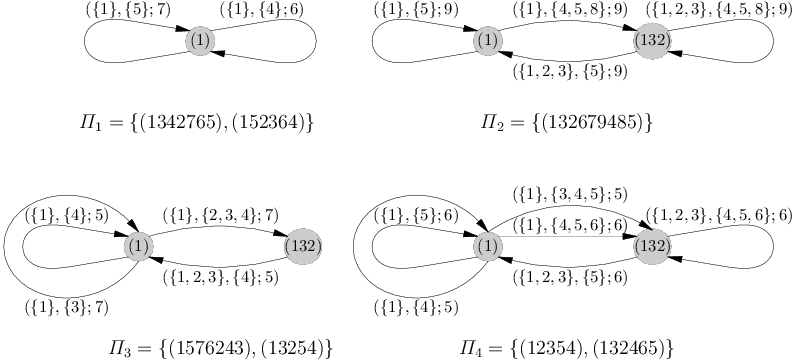
Our main technical result is as follows.
Theorem 2.2.
The graph uniquely determines the generating function .
The next corollary immediately implies Theorem 1.8.
Corollary 2.3.
Two collections of patterns and having isomorphic graphs and are strongly c-Wilf-equivalent. (Here by an ’isomorphism’ we mean a graph isomorphism preserving the labels of edges. The labels of vertices can change.)
Proof.
To prove Theorem 2.2 we present a natural algorithm calculating the number of -clusters in a given collection in terms of its graph . Namely, each vertex and a positive integer uniquely determine the subset consisting of all -clusters , such that the length of is equal to and the standardization of the initial subword of is equal to . Moreover, with each word of length (where is the length of ) one can associate the subset consisting of those clusters in which have as their initial subword. We will explain how one should compute the cardinalities of by induction on using the edge labels in . Therefore, the cardinalities of can also be computed inductively as the sums over different . Since the standardization of any word of length equals the set coincides with the set of all -clusters of length . (The cardinality of the latter set is one of required coefficients in the cluster generating function .)
Let us now return to the induction step. Take an arbitrary vertex and let …, be the list of all edges in starting at the vertex . Denote by the length of permutation labeling the vertex and denote by the length of the pattern . We present below a recurrence relation expressing the cardinality of the set in terms of the cardinalities of with the summation taken over a certain subset of words . Using this relation we can calculate inductively each and then obtain the required by summation over different . It will be convenient to subdivide the sets and into the subsets indexed by the edges starting at the vertex . For example, is the subset of -clusters formed by linkages of length between the pattern and a -cluster from . One has
| (2.4) |
Therefore, it is sufficient to find recurrence relations expressing the terms in the right-hand side of (2.4) using . To avoid very cumbersome notation let us take the case of a single edge starting at which is equivalent to fixing in the above formulas. Let be an edge in a graph coming from a pattern of length and let and be the lengths of the permutations labeling and resp. To explain our recurrence we need to introduce the following extra notation associated to .
If let be the permutation which is the inverse of the standardization of the first and the last entries of , and let be the composition of with the shifting map defined by the formula:
In other words, prescribes the rule how to write down the first and the last entries of the pattern in the increasing order:
The next statement gives the required recurrence.
Lemma 2.5.
The following relations hold:
- •
for set . Then
(2.6) - •
for one has:
(2.7)
Remark 2.8.
The range of summation in (2.6) can be easily derived from our convention on the binomial coefficients claiming that if either or . Moreover, we assume that ’s are pairwise different positive integers not exceeding . For the induction base we use the following initial data:
Proof.
We show how to prove (2.6). In formula (2.6) one has the summation over all patterns such that the word is fixed and coincides with . Indeed, the numbers are ordered by the permutation as follows: . Therefore, there are choices of entries less than among the first entries of ; there are choices of entries greater than and less than , ; there are choices of entries greater than among the first entries of ; and ways to choose the remaining standardization of the last entries of .
As an immediate consequence of Lemma 2.5 one can see that the numbers of -clusters depend only on the length, the first and the last entries of considered as sets. This justifies the information we use as the edge labels of the graph . The formulas expressing in terms of depend only on the labeling of the edges starting at . Therefore, these cardinalities can be computed by induction on using the edge labels of the graph . Finally, as we mentioned before, the set of all -clusters of length of the whole collection is equal to the set . ∎
2.1. Case of a single pattern
Let us consider separately the situation when contains just a single pattern since in this case some substantial simplifications of our construction can be done.
First of all the following observation explains why the graph is not required.
Lemma 2.9.
Let be a pattern of length and let …, be the list of all distinct lengths of possible self-linkages of , i.e. , …, is the list of distinct lengths of self-overlappings of . Then is a complete directed graph on vertices with loops and with lengths of the underlying permutations being equal to . Each ordered pair of (not necessary distinct) vertices of are connected by exactly one directed edge labeled by the corresponding initial and final subwords of .
It is obvious that and denote by () the length of the largest overlapping. Let be the standardization of the first entries of (i.e. is the labeling permutation of the -th vertex in ). Since all patterns involved in any cluster coincide with the standardization of the initial subword of any cluster should always be the same. Hence for different and fixed and all the sets coincide. Therefore, it makes sense to denote by and the cardinalities of the set of -clusters of length and those having as their initial subword resp. We introduce the same set of notation for the self-overlappings of similar to what have been using in Lemma 2.5 for the case .
Namely, for let be the permutation which is the inverse of the standardization of the first and the last entries of ; for let be the inverse of . Let be the composition using which one gets the following rearrangement of the first and last elements of in the increasing order:
Additionally, let be the standardization of the first and last entries of .
In the case of a single pattern Lemma 2.5 implies the next result.
Lemma 2.10.
For a single pattern the recurrence formula for the numbers of -clusters is as follows:
| (2.11) |
(As above we assume that the set of -clusters contains the unique fictitious element of length while the set of -clusters contains the single pattern .)
3. Application
In this section we discuss a specific class of collection of patterns. Our method from § 2 allows us to construct a system of linear ordinary differential equations in the variable for the cluster generating functions together with a set of similar generating functions associated to a given collection of patterns . The main definition is as follows.
Definition 3.1.
A collection of patterns is called monotone if for all and for each pair (not necessarily distinct) patterns from the existence of their -overlapping implies that the initial subword of the pattern does not contain entries greater than .
The next lemma explains how the monotonicity assumption simplifies the structure of the set of clusters and their generating functions.
Lemma 3.2.
Let be a linkage of a pair of patterns . Suppose that the initial subword of of length does not contain entries greater than and that the initial subword of of length does not contain entries greater than (where is the length of the overlapping of the pair in ). Then the initial subword of length of should be equal to the initial subword of , i.e. for .
Proof.
Let and be the lengths of and resp. Then the length of should be equal to . Set and respectively. The number is the minimal entry of and should be less than or equal to ( respectively). Therefore, should be the smallest entry among the first entries of the linkage and should be the smallest entry among the last entries of . In particular, . This implies that is the smallest entry in the whole and hence . Similar arguments based on simple properties of standardizations imply that is the only entry in greater than etc. ∎
Lemma 3.2 implies that for an arbitrary vertex all clusters in the subset should always have as their initial subword. This means that the number is non-vanishing if and only if , where is the length of . Consider two vertices and of lengths and connected by an edge in . We can simplify the formula (2.6) using our assumption on the intersections of clusters. At first consider the case when the length of the pattern is greater than . One observes that in this case there is no summation in (2.6) since the summands in the left-hand and the right-hand sides of (2.6) are non-vanishing if and only if for one has that and for one has that Therefore, only the last binomial coefficient in the product in the right-hand side of (2.6) is different from . Denote by the maximal entry of the final subword of . (In notation of Lemma 2.5 we have .) Since we do not have to specify the arguments of the functions the resulting recurrence relation for the cardinalities of the set of clusters is:
| (3.3) |
The case is also covered by (3.3) since in this case the maximal entry should be equal to the length of the permutation and the corresponding binomial coefficient is equal to .
Introduce the next family of generating functions:
one for each vertex of . Let …, be the list of all edges in starting at . Denote by the length of the pattern ; denote by the length of , and, finally, denote by the maximal entry among the last entries of . Formula (3.3) implies the following reccurence relation:
| (3.4) |
Theorem 3.5.
Given a monotone collection of patterns one has that the cluster generating function together with all solve the following system of linear ordinary differential equations in :
| (3.6) |
Here and runs over the set of all vertices of . (Boundary conditions for each can be easily determined in each particular case using the initial terms in (3.4).)
Proof.
Follows from (3.4). ∎
Remark 3.7.
As an immediate consequence of Theorem 3.5 one gets that satisfies a certain high order linear ordinary differential equation with polynomial coefficients (which can be obtained from the above system after the elimination of all .)
�
In particular, one can get the following simplification of the Theorem 1.8 for monotone collections of patterns.
Corollary 3.8.
Two monotone collections of patterns and are strongly c-Wilf equivalent if there exists a bijection preserving the first two properties as in Theorem 1.8 (i.e. preserving lengths and linkages) and, additionally, preserving the maxima of the overlapping sets. More precisely, for any pair of patterns of lengths and resp. and an arbitrary positive integer the coincidence of the standardizations implies the coincidence of the maxima of the sets:
(Two other sets and should coincide with the standard set because of the monotonicity property.)
With this in mind one can add two more strongly c-Wilf equivalent patterns to the pair (1.11) discussed in the introduction. Namely,
3.1. Case of a single monotone pattern
Let us present further simplifications for monotone collections with a single pattern. As it was shown in § 2.1 we do not really need the graph for collections with one pattern. Take a monotone pattern of length and let be the list of all different lengths of self-overlappings of . Let be the list of maxima among the corresponding number of the last entries of , i.e. .
Corollary 3.9.
Given a monotone pattern one has the following recurrence formula for the set of its -clusters of length :
and its cluster generating function solves the linear ordinary differential equation:
| (3.10) |
with the boundary conditions: .
Two particular cases covered by this corollary, namely the pattern and an arbitrary pattern of the form having no nontrivial self-overlappings were considered earlier in [5].
Finally, using these considerations we can completely describe which permutations of length () are c-Wilf equivalent. Our main theorem 1.8 gives necessary and sufficient condition for c-Wilf equivalence of two patterns of length . Notice that there are two natural transformations of patterns preserving the cluster generating functions. The first one is the reversion that rewrites a pattern backwards, i.e. it sends ( to ). The second one takes the complement of a pattern, i.e. it sends to . They generate the group acting on . One can easily check that this action has orbits of which orbits with representatives have length and the remaining have length . Additionally, there are 14 orbits whose permutations have no nontrivial selp-overlappings; 15 orbits with the only nontrivial self-overlapping of length ; 2 orbits with the only nontrivial self-overlapping of length , and a single orbit with self-overlappings of length 2, 3 and 4, see the lists of representatives in Proposition 3.11.
Proposition 3.11.
Subdividing the representatives of the orbits of the latter group action on into the subsets according to the lengths of their maximal possible self-overlappings one gets the following:
- •
c-Wilf equivalent orbits having no nontrivial overlappings are enumerated by their first and last elements:
- •
among all orbits with only 2-overlappings having the representatives
no two are strongly c-Wilf equivalent to each other;
- •
orbits with representatives having -overlappings are not c-Wilf equivalent;
- •
the unique orbit with overlappings of lengths is represented by the monotone pattern .
Proof.
Besides the application of Theorem 1.8 one has to check by hand that the number of -clusters is distinguishing all the 15 orbits with only 2-overlappings and already the number of -clusters distinguishes between the two orbits having only -overlappings. ∎
�
3.2. Examples of differential equations
Let us finish the paper by presenting the (system of) linear differential equations for our examples in Fig.1. One can easily check that all the collections shown there are monotone. Set and for and notice that its graph contains a single vertex. Then in the above notation one has . Equation (3.6) for the cluster generating function then takes the form:
For the collection that has self-overlappings of lengths and one has . With this data equation (3.10) takes the form:
For the collection denote its edges by , , and . Then one has ; ; ; . Thus, one gets the following system of equations:
In this case it is easy to get a linear ordinary differential equation satisfied by by dividing both sides of the first equation by , differentiating the result with respect to and equating the expressions for from the first and second equations. The resulting equation has the form
Finally, for the collection denote its edges by ; ; ; ; , and . Then one has ; ; ; ; ; . Thus, one gets the following system of equations:
Let us extract from this system a linear ordinary differential equation satisfied by . To simplify our notation set Then we get the system:
Since the coefficients in the left-hand sides are both equal to we can eliminate by differentiating the first equation a number of times and substituting from the second equation till we can solve both equations for the remaining and its derivative of appropriate order. In our concrete case, differentiating the first equation twice and substituting from the second equation we get
Differentiating the first equation in the latter system once and substituting again we get
Finally, equating the expressions for from the first equation in the latter system and from the original equation for we get the following equation
containing and its derivatives only. Substituting we obtain the required equation
for the cluster generating function.
Remark 3.12.
Notice that since the leading terms in the left-hand sides of the system (3.6) are always equal to the elimination process similar to the one just described will always lead to an equation satisfied by the cluster generating function . On the other hand, there is no guarantee that the obtained linear ordinary equation with polynomial coefficients will have the minimal possible order among such equations satisfied by .
References
- [1] R. E. L. Aldred, M. D. Atkinson, and D. J. McCaughan, Avoiding consecutive patterns in permutations. Advances in Applied Mathematics, 45 (2010), no. 3, 449-461.
- [2] V. Dotsenko, A. Khoroshkin, Anick-type resolutions and consecutive pattern avoidance. arXiv:1002.2761.
- [3] S. Elizalde Torrent, Consecutive patterns and statistics on restricted permutations. Ph.D. thesis, Universitat Politècnica de Catalunya, (2004), 170 pp.
- [4] R. Ehrenborg, S. Kitaev, and P. Perry, A Spectral Approach to Consecutive Pattern-Avoiding Permutations. arXiv:1009.2119.
- [5] S. Elizalde, M. Noy, Consecutive patterns in permutations. Formal power series and algebraic combinatorics (Scottsdale, AZ, 2001). Adv. in Appl. Math. 30 (2003), no. 1-2, 110–125.
- [6] I. P. Goulden, D. M. Jackson, An inversion theorem for cluster decompositions of sequences with distinguished subsequences. J. London Math. Soc. (2) 20 (1979), no. 3, 567–576.
- [7] S. Kitaev, A survey on partially ordered patterns. In Permutation Patterns (2010), S. Linton, N. Ruskuc, and V. Vatter, Eds., vol. 376 of London Mathematical Society Lecture Note Series, Cambridge University Press, pp. 115-135.
- [8] A. Khoroshkin, B. Shapiro, Asymptotic results in consecutive pattern avoidance of permutations, in preparation.
- [9] J. Liese and J. Remmel, Generating functions for permutations avoiding a consecutive pattern. Ann. Comb., 14 (2010) 123-141.
- [10] A. Mendes, J. Remmel, Permutations and words counted by consecutive patterns. Adv. in Appl. Math. 37 (2006), no. 4, 443–480.
- [11] J. Noonan and D. Zeilberger, The Goulden-Jackson cluster method: extensions, applications and implementations. J. Differ. Equations Appl. 5 (1999), no. 4-5, 355–377.
- [12] D. Rawlings, The q-exponential generating function for permutations by consecutive patterns and inversions. JCTA 114 (2007) 184-193.
- [13] V. A. Ufnarovskij, Combinatorial and asymptotic methods in algebra. Algebra, VI, 1–196, Encyclopaedia Math. Sci., 57, Springer, Berlin, 1995.
- [14] H. S. Wilf, The patterns of permutations. Kleitman and combinatorics: a celebration (Cambridge, MA, 1999). Discrete Math. 257 (2002), no. 2-3, 575–583.