The Straight-Line RAC Drawing Problem is NP-Hard

Let $\mathcal{Q}$ be one of quadrilaterals $\mathcal{Q}_{i}$, $i=1,2$ and let $v_{a}$, $v_{b}$, $v_{c}$ and $v_{d}$ be its vertices, consecutive along quadrilateral $\mathcal{Q}$. Assume to the contrary that vertex $v_{0}$ lies on the exterior of quadrilateral $\mathcal{Q}$ and there exists an edge, say $(v_{0},v_{a})$, that emanates from vertex $v_{0}$ towards a vertex of quadrilateral $\mathcal{Q}$, such that it crosses an edge, say $(v_{b},v_{c})$¹¹ 1 The case where, it crosses edge $(v_{c},v_{d})$ is symmetric., of quadrilateral $\mathcal{Q}$. Vertices $v_{b}$ and $v_{c}$ have the following properties: (a) they are both connected to vertex $v_{0}$, and, (b) have a common neighbor $v_{bc}$, which is incident to vertex $v_{0}$ and $v_{bc}\notin\ \mathcal{Q}$ (see Figure 1).

Observe that if vertex $v_{bc}$ lies in the non-colored regions of Figure 2, then at least one of the edges incident to $v_{bc}$ crosses either $(v_{0},v_{a})$ or $(v_{b},v_{c})$, which are already involved in a right-angle crossing. This leads to a situation where three edges mutually cross, which, by Property 1 is not permitted. Hence, vertex $v_{bc}$ should lie in the interior of the dark-gray colored regions $R_{1}$, $R_{2}$ or $R_{3}$ of Figure 2. We consider each of these cases separately in the following. Note that, there exist cases where $R_{2}\cup R_{3}=\emptyset$ (i.e., vertex $v_{0}$ is close to the intersection point of $(v_{0},v_{a})$ and $(v_{b},v_{c})$), or $R_{2}=\emptyset$ (i.e., vertex $v_{c}$ is close to the intersection point of $(v_{0},v_{a})$ and $(v_{b},v_{c})$), or $R_{3}=\emptyset$ (i.e., vertex $v_{b}$ is close to the intersection point of $(v_{0},v_{a})$ and $(v_{b},v_{c})$).

Case i:

Vertex $v_{bc}$ is in the interior of $R_{1}$. This case is depicted in Figure 3a. Let $T_{v_{bc}}$ be the region formed by vertices $v_{bc}$, $v_{b}$ and $v_{c}$ (i.e., the dark-gray colored region of Figure 3a). Vertex $v_{d}$, which has to be connected to vertices $v_{a}$ and $v_{c}$, and, the central vertex $v_{0}$, cannot lie within $T_{v_{bc}}$, since edge $(v_{a},v_{d})$ would have to cross edge $(v_{b},v_{c})$, which is already involved in a right-angle crossing. Since vertex $v_{d}$ has to be connected to vertex $v_{0}$, has to coincide with semi-line $\ell_{v_{0},v_{c},v_{bc}}^{\prime}$, as illustrated in Figure 3a. However, under this restriction, the common neighbor $v_{cd}$ of vertices $v_{c}$ and $v_{d}$ cannot be connected to vertex $v_{0}$, since edge $(v_{0},v_{cd})$ should be perpendicular to one of the edges of $T_{v_{bc}}$, which cannot be accomplished without introducing an edge overlap with edge $(v_{0},v_{d})$.

Case ii:

Vertex $v_{bc}$ is in the interior of either $R_{2}$ or $R_{3}$. Say without loss of generality that vertex $v_{bc}$ is in the interior of $R_{3}$. This case is depicted in Figure 3b. Let $u$ be a vertex of the augmented antiprism graph (except $v_{a}$) and assume that $u$ lies in the interior of the triangular face, say $T_{v_{bc}}$, formed by vertices $v_{b}$, $v_{c}$ and $v_{bc}$. Vertex $u$ has to be connected to the central vertex $v_{0}$. Edge $(v_{0},u)$ should not be involved in crossings with edges $(v_{0},v_{a})$ and $(v_{b},v_{c})$, since they are already involved in a right-angle crossing. If edge $(v_{0},u)$ crosses edge $(v_{0},v_{bc})$, then the three vertices $v_{b}$, $v_{c}$ and $v_{bc}$ that define triangle $T_{v_{bc}}$ must be collinear, which leads to a contradiction. Therefore, triangle $T_{v_{bc}}$ cannot accommodate any other vertex (except $v_{a}$). Now observe that each vertex of quadrilateral $\mathcal{Q}$ has degree five and there do not exist three vertices of quadrilateral $\mathcal{Q}$, that have a common neighbor (see Figure 1). These properties trivially hold for vertex $v_{a}$, since $v_{a}\in\mathcal{Q}$. Based on the above properties, each neighbor of vertex $v_{a}$ can lie either in the interior of the dark-gray region of Figure 3b, or, on the external face of the already constructed drawing (along the dashed semi-lines $\ell_{v_{a},v_{c},v_{bc}}^{\prime}$ and $\ell_{v_{a},v_{b},v_{bc}}^{\prime}$ of Figure 3b, respectively). This implies that we can route only four vertices out of those incident to vertex $v_{a}$, i.e., one of them should lie in the light-gray colored region of Figure 3b and thus, it cannot be connected to vertex $v_{0}$. ∎

Let $\mathcal{Q}$ be one of quadrilaterals $\mathcal{Q}_{i}$, $i=1,2$, and let, as in the previous lemma, $v_{a}$, $v_{b}$, $v_{c}$ and $v_{d}$ be its vertices, consecutive along quadrilateral $\mathcal{Q}$. Assume to the contrary that in a RAC drawing of the augmented square antiprism graph, quadrilateral $\mathcal{Q}$ is not drawn planar, and say that edges $(v_{a},v_{b})$ and $(v_{c},v_{d})$ form a right-angle crossing. This case is illustrated in Figure 4. In the following, we will lead to a contradiction the cases, where central vertex $v_{0}$ lies (i) in the interior of a triangular face of quadrilateral $\mathcal{Q}$, and, (ii) on the external face of quadrilateral $\mathcal{Q}$. Note that it is not feasible a non-planar RAC drawing of a quadrilateral to contain more than one (right-angle) crossing. Hence, its bounded faces are triangular.

• •

  Case i: Vertex $v_{0}$ lies in the interior of a triangular face of quadrilateral $\mathcal{Q}$. Assume without loss of generality that vertex $v_{0}$ (which is incident to all vertices of quadrilateral $\mathcal{Q}$) lies in the interior of the triangular face formed by vertices $v_{b}$, $v_{c}$ and the intersection point of edges $(v_{a},v_{b})$ and $(v_{c},v_{d})$, as in Figure 4a. In this case, edges $(v_{0},v_{a})$, $(v_{a},v_{b})$ and $(v_{c},v_{d})$ mutually cross, which leads to a contradiction, due to Property 1.

  

  

• •

  Case ii: Vertex $v_{0}$ lies on the external face of quadrilateral $\mathcal{Q}$. This case is illustrated in Figure 4b. Recall that by Lemma 1, vertex $v_{0}$ cannot introduce additional crossings on quadrilateral $\mathcal{Q}$. We will first show that the common neighbor $v_{ab}$ of vertices $v_{a}$ and $v_{b}$ cannot lie in the region “above” line $\ell_{v_{b},v_{c}}$. In the case, where vertex $v_{ab}$ lies in the region “above” $\ell_{v_{b},v_{c}}$ and to the “left” of both edge $(v_{c},v_{d})$ and semi-line $\ell_{v_{0},v_{d}}^{\prime}$, edge $(v_{b},v_{ab})$ would cross edge $(v_{c},v_{d})$, which is not permitted by Property 1. Symmetrically, vertex $v_{ab}$ cannot lie in the region “above” $\ell_{v_{b},v_{c}}$ and to the “right” of both edge $(v_{a},v_{b})$ and semi-line $\ell_{v_{0},v_{a}}^{\prime}$. If vertex $v_{ab}$ lies within the left gray-colored unbounded region of Figure 4b (that is formed by semi-lines $\ell_{v_{0},v_{a}}^{\prime}$, $\ell_{v_{b},v_{a}}^{\prime}$), then, edge $(v_{ab},v_{b})$ crosses two non-parallel edges $(v_{a},v_{d})$ and $(v_{a},v_{d})$. In the case where, $v_{ab}$ lies in the right gray-colored unbounded region of Figure 4b (that is formed by semi-lines $\ell_{v_{0},v_{d}}^{\prime}$, $\ell_{v_{c},v_{d}}^{\prime}$), then $(v_{a},v_{ab})$ either crosses both $(v_{a},v_{d})$ and $(v_{c},v_{d})$ which are non-parallel, or crosses edge $(v_{0},v_{d})$ forming a non-right angle crossing. In the case, where vertex $v_{ab}$ lies in the interior of the triangle formed by vertices $v_{b}$, $v_{c}$ and the intersection point of edges $(v_{a},v_{b})$ and $(v_{c},v_{d})$, edge $(v_{a},v_{ab})$ would cross edge $(v_{c},v_{d})$, which leads to a violation Property 1. Therefore, vertex $v_{ab}$ should be “below” $\ell_{v_{b},v_{c}}$.

  We continue our reasoning on vertex $v_{ab}$. Vertex $v_{ab}$ cannot lie to the “left” of edge $(v_{0},v_{a})$, since edge $(v_{b},v_{ab})$ or $(v_{a},v_{ab})$ would cross more than one (non-parallel) edges incident to vertex $v_{0}$. If vertex $v_{ab}$ lies to the “right” of edge $(v_{0},v_{b})$, then edge $(v_{a},v_{ab})$ either crosses edge $(v_{c},v_{d})$, that it is not permitted by Property 1, or, both edges $(v_{0},v_{b})$ and $(v_{0},v_{c})$, that are non-parallel. We complete our reasoning on vertex $v_{ab}$ by the triangle formed by vertices $v_{0}$, $v_{b}$ and $v_{c}$. In this case, $(v_{a},v_{ab})$ should be perpendicular to edge $(v_{0},v_{c})$. This suggests that the angle formed by edges $(v_{c},v_{d})$ and $(v_{0},v_{c})$ is greater that $180^{o}$ and therefore, edge $(v_{0},v_{d})$ either crosses $(v_{a},v_{b})$, or another edge of quadrilateral $\mathcal{Q}$, which trivially leads to a contradiction, due to Property 1, or due to Lemma 1, respectively. Based on the above, vertex $v_{ab}$ should be within the left gray-colored region of Figure 4b, along semi-line $\ell_{v_{b},v_{c},v_{0}}^{\prime}$. Following a similar reasoning scheme, as for vertex $v_{ab}$, we can prove that the common neighbor $v_{cd}$ of vertices $v_{c}$ and $v_{d}$ should lie within the right light-gray colored region of Figure 4b, along semi-line $\ell_{v_{c},v_{0},v_{b}}^{\prime}$. However, in this case, a common neighbor of vertices $v_{ab}$ and $v_{cd}$, say $v_{bc}$, should lie on the intersection of semi-lines $\ell_{v_{b},v_{0},v_{c}}^{\prime}$ and $\ell_{v_{c},v_{0},v_{b}}^{\prime}$, which leads to edge overlaps. Thus, there exists no feasible placement for vertex $v_{bc}$. ∎

From Lemma 2, it follows that quadrilateral $\mathcal{Q}_{i}$ should be drawn planar, for each $i=1,2$. In order to prove this lemma, we assume to the contrary that central vertex $v_{0}$ lies on the exterior of one of the two quadrilaterals. Say, w.l.o.g., on the exterior of quadrilateral $\mathcal{Q}_{1}$. Let $v_{a}$, $v_{b}$, $v_{c}$ and $v_{d}$ be $\mathcal{Q}_{1}$’s vertices, consecutive along quadrilateral $\mathcal{Q}_{1}$. Then, by Lemma 1, vertex $v_{0}$ cannot contribute additional crossings on quadrilateral $\mathcal{Q}_{1}$. This suggests that the drawing of the graph induced by quadrilateral $\mathcal{Q}_{1}$ and vertex $v_{0}$ will resemble the one depicted in Figure 5. We denote by $T_{v_{0}}$ the triangle formed by vertex $v_{0}$ and the two vertices, which are on the convex hall of $\mathcal{Q}_{1}$$\cup v_{0}$ (refer to the gray-colored triangle of Figure 5).

Before we proceed with the detailed proof of this lemma, we recall some properties of the augmented square antiprism graph. Two consecutive vertices of $\mathcal{Q}_{1}$ ($\mathcal{Q}_{2}$) share a common vertex of quadrilateral $\mathcal{Q}_{2}$ ($\mathcal{Q}_{1}$). Each vertex of quadrilateral $\mathcal{Q}_{1}$ ($\mathcal{Q}_{2}$) should be connected to two consecutive vertices of quadrilateral $\mathcal{Q}_{2}$ ($\mathcal{Q}_{1}$). We will prove that (i) no vertex of $\mathcal{Q}_{2}$ lies outside $T_{v_{0}}$, (ii) $\mathcal{Q}_{2}$ cannot entirely lie in the interior of $\mathcal{Q}_{1}$, (iii) $\mathcal{Q}_{2}$ cannot entirely lie in the interior of a triangular face of $T_{v_{0}}$, (iv) $\mathcal{Q}_{2}$ cannot entirely lie within two adjacent triangular faces of $T_{v_{0}}$, (v) $\mathcal{Q}_{2}$ cannot cross $\mathcal{Q}_{1}$, such that some of the vertices of $\mathcal{Q}_{2}$ reside within a triangular face of $T_{v_{0}}$, whereas the remaining ones within $\mathcal{Q}_{1}$. Note that quadrilateral $\mathcal{Q}_{2}$ cannot entirely lie within three triangular faces of $T_{v_{0}}$ incident to vertex $v_{0}$.

Case i:

We prove that no vertex of quadrilateral $\mathcal{Q}_{2}$ lies on the external face of the graph induced by quadrilateral $\mathcal{Q}_{1}$ and vertex $v_{0}$, i.e., outside $T_{v_{0}}$. For the sake of contradiction, assume that there exists a vertex of quadrilateral $\mathcal{Q}_{2}$, say $v_{ab}$, that lies on the external face of the graph induced by quadrilateral $\mathcal{Q}_{1}$ and vertex $v_{0}$ (see Figure 6). Vertex $v_{ab}$ should be connected to vertices $v_{a}$ and $v_{b}$ of quadrilateral $\mathcal{Q}_{1}$, and to the central vertex $v_{0}$. If both vertices $v_{a}$ and $v_{b}$ are inside triangle $T_{v_{0}}$, then vertex $v_{ab}$, which is assumed to lie on the external face of this graph, would violate Property 2, since vertices $v_{a}$ and $v_{b}$ would lie in the interior of $T_{v_{0}}$, whereas vertex $v_{ab}$ outside. Therefore, at least one of vertices $v_{a}$ and $v_{b}$ should be a corner of $T_{v_{0}}$. Then, vertex $v_{ab}$ contributes either none (see Figure 6b), or a single right-angle crossing (see Figure 6a).

Let now $v_{bc}$ be a vertex of quadrilateral $\mathcal{Q}_{2}$, which is incident to vertex $v_{ab}$. Vertex $v_{bc}$ is also incident to two consecutive vertices of quadrilateral $\mathcal{Q}_{1}$, i.e., $v_{b}$ and $v_{c}$. We first turn our attention in the case where $v_{ab}$ contributes a single right-angle crossing on the graph induced by quadrilateral $\mathcal{Q}_{1}$ and vertex $v_{0}$ (see Figure 6a). Then, by Property 2, vertex $v_{bc}$ should lie in the interior of triangle $T_{v_{0}}$. This immediately leads to a contradiction, since edge $(v_{ab},v_{bc})$ should cross edge $(v_{0},v_{a})$, which is already involved in a right-angle crossing (see Figure 6a).

Consider now the case where vertex $v_{ab}$ contributes no crossing on $T_{v_{0}}$. Observe that vertex $v_{bc}$, which is adjacent to vertex $v_{ab}$, vertices $v_{b}$ and $v_{c}$ of $\mathcal{Q}_{1}$, and the central vertex $v_{0}$ cannot lie in the dark-gray region of Figure 6b, since in this case, edge $(v_{a},v_{b})$ would be crossed by more than one (non-parallel) edges, incident to $v_{bc}$. The case where vertex $v_{bc}$ lies within the light-gray colored region of Figure 6b, leads to a situation similar to the one depicted in Figure 6a. Therefore, vertex $v_{bc}$ should lie “somewhere” in the interior of $T_{v_{0}}$. Let $v_{ad}$ be the common neighbor of vertices $v_{a}$ and $v_{d}$ of $\mathcal{Q}_{1}$, and vertex $v_{ab}$. This vertex cannot lie within the dark-gray region of Figure 6b, for the same reason that vertex $v_{bc}$ couldn’t. In addition, vertex $v_{ad}$ cannot lie in the interior of $T_{v_{0}}$, since in this case, both vertices $v_{bc}$ and $v_{ad}$ (that are in $T_{v_{0}}$), should be connected to $v_{ab}$ (that is not in $T_{v_{0}}$), which trivially violates Property 2. Therefore, vertex $v_{ad}$ should be on the external face of the graph induced by $\mathcal{Q}_{1}$ and vertices $v_{0}$ and $v_{ad}$, along semi-line $\ell_{v_{d},v_{0},v_{a}}^{\prime}$. However, in this case, we are also led to a situation similar to the one depicted in Figure 6a, and subsequently, to a contradiction.

Case ii:

Say that quadrilateral $\mathcal{Q}_{2}$ entirely lies within quadrilateral $\mathcal{Q}_{1}$ (see Figure 7a). In this case, its vertices should be connected to vertex $v_{0}$. For three vertices of quadrilateral $\mathcal{Q}_{2}$, this can be accomplished using the three available edges of quadrilateral $\mathcal{Q}_{1}$ (refer to the dotted edges of Figure 7a), such that the right-angle crossings occur along them. However, the fourth vertex cannot be connected to vertex $v_{0}$, since only three edges of quadrilateral $\mathcal{Q}_{1}$ can be used to realize connections with vertex $v_{0}$ (see the topmost edge of Figure 7a).

Case iii:

Assume now that quadrilateral $\mathcal{Q}_{2}$ entirely lies within a triangular face, say $T_{Q_{1}}$, incident to vertex $v_{0}$ (see Figure 7b). Then, there exists at least one vertex of quadrilateral $\mathcal{Q}_{1}$, say vertex $q$, which is incident to two vertices of quadrilateral $\mathcal{Q}_{2}$, and is not identified with a vertex at the corners of $T_{Q_{1}}$ (see Figure 7b). Vertex $q$ has to be connected to two vertices of quadrilateral $\mathcal{Q}_{2}$. However, vertex $q$ is external to triangle $T_{Q_{1}}$, whereas its two incident vertices in the interior of this triangle, which leads to a violation of Property 2.

Case iv:

Say that quadrilateral $\mathcal{Q}_{2}$ entirely lies within two adjacent triangular faces, say $T_{Q_{1}}^{1}$ and $T_{Q_{1}}^{2}$, incident to vertex $v_{0}$ (see Figure 7c). Then, quadrilateral $\mathcal{Q}_{2}$ should be “perpendicular” to the common edge of $T_{Q_{1}}^{1}$ and $T_{Q_{1}}^{2}$. Recall that two consecutive vertices of quadrilateral $\mathcal{Q}_{2}$ share a common vertex of quadrilateral $\mathcal{Q}_{1}$. Hence, we can find a vertex $q$ of quadrilateral $\mathcal{Q}_{1}$, which is not identified with the common vertex of $T_{Q_{1}}^{1}$ and $T_{Q_{1}}^{2}$, and is incident to a pair of vertices of quadrilateral $\mathcal{Q}_{2}$, that do not lie in the same triangular face (i.e., the topmost vertices of quadrilateral $\mathcal{Q}_{2}$ or the bottommost vertices of quadrilateral $\mathcal{Q}_{2}$ in Figure 7c). This leads to a contradiction, since the common edge of $T_{Q_{1}}^{1}$ and $T_{Q_{4}}^{2}$ cannot be crossed, as it is already involved in a right-angle crossing (refer to the dotted-edges of Figure 7c).

Case v:

We consider the case where quadrilateral $\mathcal{Q}_{2}$ crosses quadrilateral $\mathcal{Q}_{1}$, such that some of the vertices of quadrilateral $\mathcal{Q}_{2}$ reside within a triangular face of $T_{v_{0}}$, whereas the remaining ones within quadrilateral $\mathcal{Q}_{1}$. We will lead to a contradiction the cases where: (i) Two vertices of $\mathcal{Q}_{2}$ lie in the interior of a single triangular face incident to $v_{0}$, (ii) two vertices of $\mathcal{Q}_{2}$ lie in the interior of two adjacent triangular faces, (iii) three vertices of $\mathcal{Q}_{2}$ lie in the interior of two adjacent triangular faces and two of them lie in the same triangular face of $T_{v_{0}}$, (iv) three vertices of $\mathcal{Q}_{2}$ lie in the interior of three pairwise-adjacent triangular faces incident to vertex $v_{0}$. Recall that none of the vertices of $\mathcal{Q}_{2}$ lies in the external face of the graph induced by quadrilateral $\mathcal{Q}_{1}$ and vertex $v_{0}$. Let, with a slight abuse of notation, $q_{a}$, $q_{b}$, $q_{c}$ and $q_{d}$ be the vertices of quadrilateral $\mathcal{Q}_{2}$. Assume first that vertices $q_{a}$ and $q_{b}$ are in the interior of a single triangular face, whereas vertices $q_{c}$ and $q_{d}$ in the interior of quadrilateral $\mathcal{Q}_{1}$ (see Figure 8). In this case, edges $(q_{a},q_{d})$ and $(q_{b},q_{c})$ should perpendicularly cross quadrilateral $\mathcal{Q}_{1}$. The connections between vertices $q_{c}$ and $q_{d}$ with vertex $v_{0}$ can be accomplished using two of the available edges of quadrilateral $\mathcal{Q}_{1}$, such that the right-angle crossings occur along them (refer to dotted edges of Figure 8). Thus, the triangular faces that are adjacent to the one that accommodates vertices $q_{a}$ and $q_{b}$ (refer to the light-gray faces of Figure 8) cannot be further used to connect vertices of quadrilateral $\mathcal{Q}_{1}$ to vertices of quadrilateral $\mathcal{Q}_{2}$. Then, there exists a vertex of quadrilateral $\mathcal{Q}_{1}$, say $q$, that it is not identified with any of the vertices of the face that accommodates vertices $q_{a}$ and $q_{b}$, and either $q_{a}$ or $q_{b}$ has to be connected to vertex $q$. However, this cannot be accomplished, since the edge from either $q_{a}$ or $q_{b}$ to vertex $q$ would cross more than one non-parallel edges (refer to the dashed edge of Figure 8).

Say now that vertices $q_{a}$ and $q_{b}$ are in the interior of two adjacent triangular faces incident to vertex $v_{0}$, whereas vertices $q_{c}$ and $q_{b}$ within quadrilateral $\mathcal{Q}_{1}$. This case is illustrated in Figure 9a. Then, one of the vertices that lie in the interior of quadrilateral $\mathcal{Q}_{1}$, say vertex $q_{d}$, can be connected to vertex $v_{0}$ using one of the available edges of quadrilateral $\mathcal{Q}_{1}$ (refer to the dotted edge of Figure 9a). However, vertex $q_{c}$ cannot be connected to vertex $v_{0}$, since only three of the edges of quadrilateral $\mathcal{Q}_{1}$ can be used to realize connections from the vertices that lie within quadrilateral $\mathcal{Q}_{1}$, to vertex $v_{0}$.

Consider now the case where three vertices, say $q_{a}$, $q_{b}$ and $q_{c}$ of quadrilateral $\mathcal{Q}_{2}$ are in the interior of two adjacent triangular faces incident to vertex $v_{0}$, and two of vertices $q_{a}$, $q_{b}$ and $q_{c}$, say w.l.o.g., $q_{b}$ and $q_{c}$, lie in the same triangular face (see Figure 9b). Then, vertex $q_{d}$, as in the previous case, can be connected to vertex $v_{0}$ using the “last” available edge of quadrilateral $\mathcal{Q}_{1}$ (refer to the dotted edge of Figure 9b). However, in this case, there exists a vertex of quadrilateral $\mathcal{Q}_{1}$, say $q$, that it is not identified with any of the vertices of the face that accommodates vertices $q_{a}$, $q_{b}$ and $q_{c}$, which has to be connected to one of the vertices $q_{a}$, $q_{b}$ or $q_{c}$. However, this cannot be accomplished, since an edge from either vertex $q_{a}$, or $q_{b}$, or $q_{c}$, to vertex $q$ would cross more than one non-parallel edges (refer to the dashed edge of Figure 9b).

The last case we have to consider is the one where three vertices, say $q_{a}$, $q_{b}$ and $q_{c}$ of quadrilateral $\mathcal{Q}_{2}$ are in the interior of three pairwise-adjacent triangular faces incident to vertex $v_{0}$, whereas the fourth vertex $q_{d}$ resides within quadrilateral $\mathcal{Q}_{2}$ (see Figure 9c). In this case, vertex $q_{d}$ has to use the fourth edge of quadrilateral $\mathcal{Q}_{1}$ to reach vertex $v_{0}$, which leads to a contradiction, since only three of the edges of quadrilateral $\mathcal{Q}_{1}$ can be used to realize connections from the vertices that lie within quadrilateral $\mathcal{Q}_{1}$, to vertex $v_{0}$.

Thus, we have considered all possible placements of $\mathcal{Q}_{2}$, with vertex $v_{0}$ outside of $\mathcal{Q}_{1}$, and are all led to a contradiction. We conclude that vertex $v_{0}$ is in the interior of quadrilateral $\mathcal{Q}_{1}$ (and symmetrically in the interior of $\mathcal{Q}_{2}$, too). ∎

By Lemma 3, vertex $v_{0}$ should lie in the interior of quadrilateral $\mathcal{Q}_{i}$, $i=1,2$, which is drawn planar due to Lemma 2. Assume to the contrary that in a RAC drawing of the augmented square antiprism graph, an edge emanating from vertex $v_{0}$ towards a vertex of quadrilateral $\mathcal{Q}_{1}$, say $v_{a}$, crosses an edge, say $(v_{c},v_{d})$, of quadrilateral $\mathcal{Q}_{1}$ (see Figure 10). Consider vertex $v_{cd}$, which is incident to vertices $v_{c}$ and $v_{d}$ of quadrilateral $\mathcal{Q}_{2}$. Vertex $v_{cd}$ cannot lie “above” line $\ell_{v_{c},v_{d}}$ and to the “left” of semi-line $\ell_{v_{d},v_{a}}^{\prime}$, since it cannot be connected to vertex $v_{0}$. In addition, it cannot lie “above” line $\ell_{v_{c},v_{d}}$ and to the “right” of semi-line $\ell_{v_{d},v_{a}}^{\prime}$, since in this case it cannot be connected to either vertex $v_{c}$ or $v_{0}$. Furthermore, vertex $v_{cd}$ cannot be in the interior of the triangle formed by vertices $v_{0}$, $v_{c}$ and $v_{d}$, as it would not be feasible to be connected either to vertex $v_{c}$ or $v_{d}$, since in either case, it crosses edge $(v_{0},v_{a})$. Also, $v_{cd}$ cannot be in the region formed by line $\ell_{v_{c},v_{d}}$ and edges $(v_{0},v_{d})$ and $(v_{0},v_{b})$, as it could not be connected to vertex $v_{c}$. Thus, vertex $v_{cd}$ should lie in the light-gray triangular face of Figure 10, along semi-line $\ell_{v_{d},v_{c},v_{b}}$. Following a similar reasoning scheme, we can prove that vertex $v_{ad}$, which is incident to vertices $v_{a}$, $v_{d}$ of quadrilateral $\mathcal{Q}_{1}$ and vertex $v_{ab}$ of quadrilateral $\mathcal{Q}_{2}$, due to its adjacency with $v_{a}$, $v_{d}$, can lie in the face formed by vertices $v_{a}$, $v_{b}$, $v_{d}$ and the intersection point of edges $(v_{d},v_{cd})$ and $(v_{0},v_{b})$. However, under this restriction, vertex $v_{ad}$ cannot be connected to vertex $v_{cd}$, without crossing edge $(v_{0},v_{b})$, which is already involved in a right-angle crossing (refer to the dashed edge of Figure 10). ∎

From Lemmata 2, 3 and 4, it follows that the graph induced by quadrilateral $\mathcal{Q}_{1}$ and vertex $v_{0}$ is drawn planar with vertex $v_{0}$ in the interior of both quadrilaterals $\mathcal{Q}_{1}$ and $\mathcal{Q}_{2}$. Therefore, it should resemble the one illustrated in Figure 11a.

In order to prove this lemma, we will contradict the following cases: (i) $\mathcal{Q}_{1}$ and $\mathcal{Q}_{2}$ cross and none of the vertices of $\mathcal{Q}_{2}$ is in the interior of quadrilateral $\mathcal{Q}_{1}$, (ii) two vertices of $\mathcal{Q}_{2}$ lie in the interior of $\mathcal{Q}_{1}$ and $\mathcal{Q}_{2}$ crosses either a single edge of $\mathcal{Q}_{1}$, or two edges of $\mathcal{Q}_{1}$, (iii) three vertices of $\mathcal{Q}_{2}$ lie in the interior of $\mathcal{Q}_{1}$, (iv) only one vertex of $\mathcal{Q}_{2}$ lies in the interior of $\mathcal{Q}_{1}$. We first assume that quadrilateral $\mathcal{Q}_{1}$ and quadrilateral $\mathcal{Q}_{2}$ cross and none of the vertices of quadrilateral $\mathcal{Q}_{2}$ is in the interior of quadrilateral $\mathcal{Q}_{1}$ (see Figure 11b). In this case, an edge of quadrilateral $\mathcal{Q}_{2}$, say $e_{q}$, which is involved in the crossing, divides quadrilateral $\mathcal{Q}_{1}$ into two regions, say $\mathcal{Q}_{1}^{1}$ and $\mathcal{Q}_{1}^{2}$. Obviously, edge $e_{q}$ should cross parallel edges of quadrilateral $\mathcal{Q}_{1}$. Then, vertex $v_{0}$, which lies in the interior of quadrilateral $\mathcal{Q}_{1}$ and is incident to all vertices of quadrilateral $\mathcal{Q}_{1}$ cannot reside to none of $\mathcal{Q}_{1}^{1}$ and $\mathcal{Q}_{1}^{2}$, without introducing a non-right angle crossing with edge $e_{q}$.

We proceed to consider the case where quadrilaterals $\mathcal{Q}_{1}$ and $\mathcal{Q}_{2}$ cross and some of the vertices of quadrilateral $\mathcal{Q}_{2}$ are in the interior of quadrilateral $\mathcal{Q}_{1}$, whereas the remaining ones on its exterior. Let $q_{a}$, $q_{b}$, $q_{c}$ and $q_{d}$ be the vertices of quadrilateral $\mathcal{Q}_{2}$. Assume that $q_{a}$ and $q_{b}$ lie within quadrilateral $\mathcal{Q}_{1}$, whereas $q_{c}$ and $q_{d}$ on its external face, such that edges $(q_{a},q_{d})$ and $(q_{b},q_{c})$ are perpendicular either to one edge of quadrilateral $\mathcal{Q}_{1}$ (see Figure 12a), or to two edges of $\mathcal{Q}_{1}$ (see Figure 12b). Note that edges $(q_{a},q_{d})$ and $(q_{b},q_{c})$ cannot be crossed by any other edge incident to both quadrilaterals, since they are already involved in right-angle crossings. However, all vertices of quadrilateral $\mathcal{Q}_{1}$ have to be connected to vertex $v_{0}$. Assuming that one vertex of quadrilateral $\mathcal{Q}_{1}$ can utilize the “last” available edge of quadrilateral $\mathcal{Q}_{2}$ (i.e., edge $(q_{a},q_{b})$) to reach vertex $v_{0}$ (refer to the dotted edges of Figures 12a and 12b), there exists at least one vertex of $\mathcal{Q}_{1}$, say vertex $q$, that cannot be connected to $v_{0}$, without introducing non right-angle crossing (refer to the dashed edges of Figures 12a and 12b).

Following a similar reasoning scheme as for the previous cases, we can prove that the cases where (i) three vertices of $\mathcal{Q}_{2}$, say w.l.o.g., $q_{a}$, $q_{b}$ and $q_{c}$, lie in the interior of $\mathcal{Q}_{1}$ (see Figure 13a) , and (ii) only one vertex of $\mathcal{Q}_{2}$, say w.l.o.g, vertex $q_{b}$, lies in the interior of $\mathcal{Q}_{1}$ (see Figure 13b), are led to a contradiction. ∎

So far, we have managed to prove that both quadrilaterals $\mathcal{Q}_{1}$ and $\mathcal{Q}_{2}$ are drawn planar, do not cross, and have central vertex $v_{0}$ to their interior. This suggests that either quadrilateral $\mathcal{Q}_{1}$ is in the interior of $\mathcal{Q}_{2}$, or quadrilateral $\mathcal{Q}_{2}$ is in the interior of $\mathcal{Q}_{1}$. However, in both cases, vertex $v_{0}$, which has to be connected to the four vertices of the “external” quadrilateral, should inevitably perpendicularly cross the four edges of the “internal” quadrilateral, and this trivially implies only two feasible combinatorial embeddings. ∎

Assume first that in a RAC drawing of $G\oplus G^{\prime}$, vertices $v$ and $v^{\prime}$ are on the external quadrilateral of $G$ and graph $G^{\prime}$ is drawn completely in the interior of $G$ (see Figure 14b; since $v$ and $v^{\prime}$ are on the external face of $G^{\prime}$, vertices $\alpha$ and $\beta$ in Figure 14b should also be on the external face of $G^{\prime}$). First observe that vertex $u^{\prime}$ of $G^{\prime}$, which is incident to vertices $v$ and $v^{\prime}$, cannot reside to the “left” of both edges $(u,v)$ and $(u,v^{\prime})$ (refer to the bold drawn edges of Figure 14b), since this would lead to a situation where three edges mutually cross and, subsequently, to a violation of Property 1 (see the gray-colored square vertex of Figure 14b). Therefore, vertex $u^{\prime}$ should lie within the triangular face of $G$ formed by vertices $u$, $v$ and $v^{\prime}$. The same similarly holds for the central vertex of $G^{\prime}$, which is also incident to vertices $v$ and $v^{\prime}$. By Property 2, any common neighbor of vertices $u^{\prime}$ and $v$ should also lie within the same triangular face of $G$, which progressively implies that entire graph $G^{\prime}$ should reside within this face, as in Figure 14b. However, in this case and since $u^{\prime}$ is incident to $v$ and $v^{\prime}$, edge $(u,u^{\prime})$, which is used on a horizontal or a vertical extension, crosses the interior of $G^{\prime}$, which is not permitted. This suggests that graph $G^{\prime}$ should be on the exterior of $G$.

Now assume that vertices $v$ and $v^{\prime}$, which are identified, during a horizontal or vertical extension, are along the internal quadrilateral of $G$ in a RAC drawing of $G\oplus G^{\prime}$. This is illustrated in Figure 14c. Then, the edge, say $e$, which perpendicularly crosses edge $(v,v^{\prime})$ and emanates from the external quadrilateral towards the central vertex of $G$ (refer to the bold solid edge of Figure 14c) will be involved in crossings with $G^{\prime}$. More precisely, we focus on vertex $u^{\prime}$ of $G^{\prime}$, which is incident to vertices $v$ and $v^{\prime}$. These edges will inevitably introduce non-right angle crossings, since one of them should cross edge $e$. Therefore, the vertices that are identified, during a horizontal or vertical extension, should always be on the external face of each augmented square antiprism graph and, subsequently, the drawing of the graph produced by a horizontal or vertical extension will resemble the one of Figure 14a, i.e., it has a unique embedding. ∎

We will reduce the well-known $3$-SAT problem [11] to the straight-line RAC drawing problem. In a $3$-SAT instance, we are given a formula $\phi$ in conjunctive normal form with variables $x_{1},x_{2},\ldots,x_{n}$ and clauses $C_{1},C_{2},\ldots,C_{m}$, each with three literals. We show how to construct a graph $G_{\phi}$ that admits a straight-line RAC drawing $\Gamma(G_{\phi})$ if and only if formula $\phi$ is satisfiable.

Figure 15 illustrates the gadgets of our construction. Each gray-colored square in these drawings corresponds to an augmented square antiprism graph. Adjacent gray squares form an extension (refer, for example, to the topmost gray squares of Figure 15a, which form a “horizontal” extension). There also exist gray squares that are not adjacent, but connected with edges. The legend in Figure 15 describes how the connections are realized.

The gadget that encodes variable $x_{i}$ of formula $\phi$ is given in Figure 15a. The gadget of variable $x_{i}$ consists of a combination of augmented square antiprism graphs, and, “horizontal” and “vertical” edges, which form a tower, whose RAC drawing has unique combinatorial embedding. One side of the tower accommodates multiple vertices that correspond to literal $x_{i}$, whereas its opposite side accommodates vertices that correspond to literal $\overline{x_{i}}$ (refer to vertices $x_{i,1},\ldots,x_{i,m}$ and $\overline{x}_{i,1},\ldots,\overline{x}_{i,m}$ in Figure 15a). These vertices are called variable endpoints. Then, based on whether on the final drawing the negated vertices will appear to the “left” or to the “right” side of the tower, we will assign a true or a false value to variable $x_{i}$, respectively. Pairs of consecutive endpoints $x_{i,j}$ and $x_{i,j+1}$ are separated by a corridor (see Figure 15a), which allows perpendicular edges to pass through it (see the bottommost dashed arrow of Figure 15a). Note that this is not possible through a “corridor” formed on a variable endpoint, since there exist four non-parallel edges that “block” any other edge passing through them (see the topmost dashed arrow of Figure 15a). The corridors can have variable height. In the variable gadget of variable $x_{i}$, there are also two vertices (they are drawn as gray circles in Figure 15a), which have degree four. These vertices serve as “connectors” among consecutive variable gadgets, i.e., these vertices should be connected to their corresponding vertices on the variable gadgets of variables $x_{i-1}$ and $x_{i+1}$. Note that the connector vertices of the variable gadgets associated with variables $x_{1}$ and $x_{n}$ are connected to connectors of the variable gadgets that correspond to variables $x_{2}$ and $x_{n-1}$, respectively, and to connectors of dummy variable gadgets.

Figure 15b illustrates a dummy variable gadget, which (similarly to the variable gadget) consists of a combination of augmented square antiprism graphs, and, “horizontal” and “vertical” edges, which form a tower. Any RAC drawing of this gadget has also unique combinatorial embedding. A dummy variable gadget does not support vertices that correspond to literals. However, it contains connector vertices (they are drawn as gray circles in Figure 15b). In our construction, we use exactly two dummy variable gadgets. The connector vertices of each dummy variable gadget should be connected to their corresponding connector vertices on the variable gadgets associated with variables $x_{1}$ and $x_{n}$, respectively.

The gadget that encodes the clauses of formula $\phi$ is illustrated in Figure 15c and resembles to a valve. Let $C_{i}=(x_{j}\vee x_{k}\vee x_{l})$ be a clause of $\phi$. As illustrated in Figure 15c, the gadget which corresponds to clause $C_{i}$ contains three vertices²² 2 With slight abuse of notation, the same term is used to denote variables of $\phi$ and vertices of $G_{\phi}$., say $x_{j}$, $x_{k}$, and $x_{l}$, such that: $x_{j}$ has to be connected to $x_{j,i}$, $x_{k}$ to $x_{k,i}$ and $x_{l}$ to $x_{l,i}$ by paths of length two. These vertices, referred to as the clause endpoints, encode the literals of each clause. Obviously, if a clause contains a negated literal, it should be connected to the negated endpoint of the corresponding variable gadget. The clause endpoints are incident to a vertex “trapped” within two parallel edges (refer to the bold drawn edges of Figure 15c). Therefore, in a RAC drawing of $G_{\phi}$, only two of them can perpendicularly cross these edges, one from top (top endpoint) and one from bottom (bottom endpoint). The other one (right endpoint) should remain in the interior of the two parallel edges. The one that will remain “trapped” on the final drawing will correspond to the true literal of this clause.

The gadgets, which correspond to variables and clauses of $\phi$, are connected together by the skeleton of graph $G_{\phi}$, which is depicted in Figure 16a. The skeleton consists of two main parts, i.e., one “horizontal” and one “vertical”. The vertical part accommodates the clause gadgets (see Figure 16a). The horizontal part will be used in order to “plug” the variable gadgets. The long edges that perpendicularly cross (refer to the crossing edges slightly above the horizontal part in Figure 16a), imply that the vertical part should be perpendicular to the horizontal part. The horizontal part of the skeleton is separately illustrated in Figure 16b. Observe that it contains one set of horizontal lines.

Figure 17 shows how the variable gadgets are attached to the skeleton. More precisely, this is accomplished by a single edge, which should perpendicularly cross the set of the horizontal edges of the horizontal part. Therefore, each variable gadget is perpendicularly attached to the skeleton, as in Figure 17. Note that each variable gadget should be drawn completely above of these horizontal edges, since otherwise the connections among variable endpoints and clause endpoints would not be feasible. The connector vertices of the dummy variable gadgets, the variable gadgets and the vertical part of the construction, ensure that the variable gadgets will be parallel to each other (i.e., they are not allowed to bend) and parallel to the vertical part of the construction.

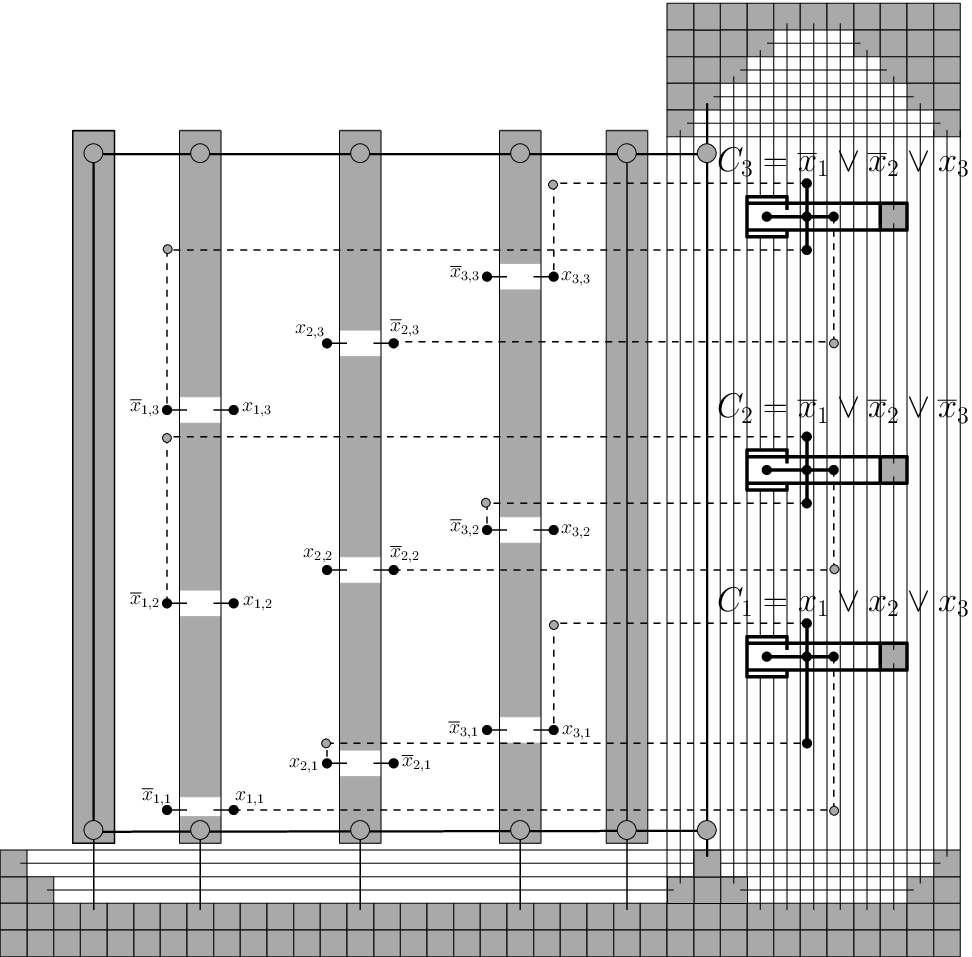
We now proceed to investigate some properties of our construction. Any path of length two that emanates from a top- or bottom-clause endpoint can reach a variable endpoint either on the left or on the right side of its associated variable gadget. The first edge of this path should perpendicularly cross the vertical edges of the vertical part of the construction and pass through some corridors³³ 3 In Figure 17, the corridors are the gray-colored regions that reside at each variable gadget., whereas the second edge will be used to realize the “final” connection with the variable gadget endpoint (see Figure 17). However, the same doesn’t hold for the paths that emanate from a right-clause endpoint. These paths can only reach variable endpoints on the right side of their associated variable gadgets. More precisely, the first edge of the $2$-length path should cross one of the two parallel edges (refer to the bold drawn edges of Figure 15c) that “trap” it, whereas the other one should be used to reach (passing through variable corridors) its variable endpoint (see Figure 17).

Our construction ensures that up to translations, rotations and stretchings any RAC drawing of $G_{\phi}$ resembles the one of Figure 16. It is clear that the construction can be completed in $O(nm)$ time. Assume now that there is a RAC drawing $\Gamma(G_{\phi})$ of $G_{\phi}$. If the negated vertices of the variable gadget that corresponds to $x_{i}$, $i=1,2,\ldots,n$, lie to the “left” side in $\Gamma(G_{\phi})$, then variable $x_{i}$ is set to true, otherwise $x_{i}$ is set to false. We argue that this assignment satisfies $\phi$. To realize this, observe that there exist three paths that emanate from each clause gadget. The one that emanates from the right endpoint of each clause gadget can never reach a false value. Therefore, each clause of $\phi$ must contain at least one true literal, which implies that $\phi$ is satisfiable.

Conversely, suppose that there is a truth assignment that satisfies $\phi$. We proceed to construct a RAC drawing $\Gamma(G_{\phi})$ of $G_{\phi}$, as follows: In the case where, in the truth assignment, variable $x_{i}$, $i=1,2,\ldots,n$ is set to true, we place the negated vertices of the variable gadget that corresponds to $x_{i}$, to its left side in $\Gamma(G_{\phi})$, otherwise to its right side. Since each clause of $\phi$ contains at least one true literal, we choose this as the right endpoint of its corresponding clause gadget. As mentioned above, it is always feasible to be connected to its variable gadgets by paths of length two. This completes our proof. ∎

References

- [1] Angelini, P., Cittadini, L., Di Battista, G., Didimo, W., Frati, F., Kaufmann, M., Symvonis, A.: On the perspectives opened by right angle crossing drawings. In: Proc. of 17th International Sympsioum on Graph Drawing (GD09). LNCS, vol. 5849, pp. 21–32 (2009)
- [2] Argyriou, E.N., Bekos, M.A., Symvonis, A.: Maximizing the total resolution of graphs. In: Proc. of 18th International Sympsioum on Graph Drawing (GD10) (2010), to appear
- [3] Arikushi, K., Fulek, R., Keszegh, B., Moric, F., Toth, C.: Drawing graphs with orthogonal crossings. In: Proc. 36th International Workshop on Graph Theoretic Concepts in Computer Science (WG 2010) (2010), to appear
- [4] Battista, G.D., Eades, P., Tamassia, R., Tollis, I.G.: Algorithms for drawing graphs: an annotated bibliography. Compututational Geometry 4, 235–282 (1994)
- [5] Bodlaender, H.L., Tel, G.: A note on rectilinearity and angular resolution. Journal of Graph Algorithms and Applications 8, 89–94 (2004)
- [6] Di Giacomo, E., Didimo, W., Liotta, G., Meijer, H.: Area, curve complexity, and crossing resolution of non-planar graph drawings. In: Proc. of 17th International Sympsioum on Graph Drawing (GD09). LNCS, vol. 5849, pp. 15–20 (2009)
- [7] Didimo, W., Eades, P., Liotta, G.: Drawing graphs with right angle crossings. In: Proc. of 12th International Symposium, Algorithms and Data Structures (WADS09). LNCS, vol. 5664, pp. 206–217 (2009)
- [8] Didimo, W., Eades, P., Liotta, G.: A characterization of complete bipartite graphs. Information Processing Letters 110(16), 687–691 (2010)
- [9] Dujmovic, V., Gudmundsson, J., Morin, P., Wolle, T.: Notes on large angle crossing graphs. In: Computing: Theory of Computing 2010. Australian Computer Society (2010)
- [10] Formann, M., Hagerup, T., Haralambides, J., Kaufmann, M., Leighton, F., Symvonis, A., Welzl, E., Woeginger, G.: Drawing graphs in the plane with high resolution. SIAM Journal of Computing 22(5), 1035–1052 (1993)
- [11] Garey, M.R., Johnson, D.S.: Computers and Intractability: A Guide to the Theory of NP-Completeness. W. H. Freeman (1979)
- [12] Garey, M., Johnson, D.: Crossing number is NP-complete. SIAM Journal of Algebraic Discrete Methods 4, 312–316 (1983)
- [13] Garg, A., Tamassia, R.: Planar drawings and angular resolution: Algorithms and bounds (extended abstract). In: Proc. 2nd Annual European Symposium on Algorithms. pp. 12–23 (1994)
- [14] Gutwenger, C., Mutzel, P.: Planar polyline drawings with good angular resolution. In: Proc. of 6th International Symposium on Graph Drawing. LNCS, vol. 1547, pp. 167–182 (1998)
- [15] Huang, W.: Using eye tracking to investigate graph layout effects. Asia-Pacific Symposium on Visualization pp. 97–100 (2007)
- [16] Huang, W., Hong, S.H., Eades, P.: Effects of crossing angles. In: PacificVis. pp. 41–46 (2008)
- [17] Kaufmann, M., Wagner, D. (eds.): Drawing Graphs: Methods and Models, LNCS, vol. 2025. Springer-Verlag (2001)
- [18] van Kreveld, M.: The quality ratio of RAC drawings and planar drawings of planar graphs. In: Proc. of 18th International Sympsioum on Graph Drawing (GD10) (2010), to appear
- [19] Lin, C.C., Yen, H.C.: A new force-directed graph drawing method based on edge-edge repulsion. In: Proc. of the 9th International Conference on Information Visualization. pp. 329–334. IEEE (2005)
- [20] Malitz, S.M., Papakostas, A.: On the angular resolution of planar graphs. In: Proc. of the 24th Annual ACM Symposium on Theory of Computing (STOC92). pp. 527–538. ACM (1992)
- [21] Purchase, H.C.: Effective information visualisation: a study of graph drawing aesthetics and algorithms. Interacting with Computers 13(2), 147–162 (2000)
- [22] Purchase, H.C., Carrington, D.A., Allder, J.A.: Empirical evaluation of aesthetics-based graph layout. Empirical Software Engineering 7(3), 233–255 (2002)
- [23] Ware, C., Purchase, H., Colpoys, L., McGill, M.: Cognitive measurements of graph aesthetics. Information Visualization 1(2), 103–110 (2002)