Next-to-next-to-leading soft-gluon corrections for the top quark cross section and transverse momentum distribution
Nikolaos Kidonakis
Kennesaw State University, Physics #1202,
1000 Chastain Rd., Kennesaw, GA 30144-5591, USA
Abstract
I present results for top quark production in hadronic collisions at LHC and Tevatron energies. The soft-gluon corrections to the differential cross section are resummed at next-to-next-to-leading-logarithm (NNLL) accuracy via the two-loop soft anomalous dimension matrices. Approximate next-to-next-to-leading-order (NNLO) differential and total cross sections are calculated. Detailed theoretical predictions are shown for the cross section and the top quark distribution at the Tevatron and the LHC.
1 Introduction
The top quark occupies a unique position in the list of elementary particles as the most massive particle discovered to date. Its high mass suggests an important role for the top quark in the physics of electroweak symmetry breaking. After a long period of searches, the discovery of the top quark via top-antitop production in proton-antiproton collisions () was announced in 1995 by the CDF and D0 collaborations at the Fermilab Tevatron collider [1]. The cross section has been measured with increasing precision at Run II of the Tevatron [2, 3] and there has also been data for the transverse momentum, , distribution of the top quark [4]. More recently single top quark production was observed by D0 [5] and CDF [6]. Measurements of the top quark mass have also been increasingly more precise [7]. The LHC is expected to observe a very large number of top quark events and to bring top quark physics to a new energy frontier. For reviews of top quark physics at the Tevatron and the LHC see Ref. [8] (experiment) and Ref. [9] (theory).
The experimental measurements of the top quark cross section and distribution at the Tevatron are currently in good agreement with theoretical predictions. However, as the experimental errors continue to get smaller with time, precise theoretical calculations with smaller uncertainties are required. Next-to-leading order (NLO) calculations of the QCD corrections have been available for over two decades [10, 11] (electroweak corrections, which are much smaller numerically, have also been calculated more recently [12]) but the associated uncertainty is much bigger than current experimental errors. The inclusion of higher-order soft-gluon corrections enhances the cross section and distribution and significantly reduces the theoretical error [13, 14].
Until recently, the state of the art in theoretical predictions was approximate next-to-next-to-leading order (NNLO) calculations based on next-to-leading-logarithm (NLL) resummation of soft-gluon corrections for the differential cross section, supplemented with further subleading terms [13, 14]. These soft-gluon corrections are dominant not only near partonic threshold but also away from it. The accuracy at NLL was achieved by the calculation of the one-loop soft anomalous dimension matrices for the partonic channels in top quark production in Ref. [15].
To achieve next-to-next-to-leading-logarithm (NNLL) accuracy in the resummation one needs to calculate the soft anomalous dimensions at two loops. This is a much more difficult undertaking. For massless quark scattering, the two-loop soft anomalous dimension matrix was first calculated in Ref. [16]. Further work on soft and collinear singularities of dimensionally-regularized scattering amplitudes in massless gauge theories followed in Refs. [17, 18, 19, 20, 21]. More recently, a lot of work on massive two-loop soft anomalous dimensions has appeared in Refs. [22, 23, 24, 25, 26, 27, 28, 29, 30, 31, 32]. The presence of a mass for the top quark considerably complicates the calculation relative to the massless case.
Soft-gluon resummation is a consequence of factorization. The partonic cross section can be factorized into functions associated with the hard scattering, collinear and soft-gluon emission from the external partons, and noncollinear soft-gluon emission that depends on the color structure of the process [15]. The renormalization group evolution of these functions results in expressions for the resummed cross section. The resummation formalism followed here has already been presented and reviewed in numerous papers over a period of more than a decade (see Refs. [13, 15, 28, 29, 33, 34, 35] and references therein) so we will not repeat the derivation of resummation and we will not repeat explicit expressions in this paper except for new two-loop results in Section 2. Resummation is performed in Mellin moment space: we define a kinematical variable that measures distance from partonic threshold, and then is the moment variable conjugate to . For production the resummed partonic cross section in moment space is given by
| (1.1) |
The first exponent in the above expression resums soft and collinear corrections from the incoming partons and (quark-antiquark or gluon-gluon) while the second exponent controls the factorization scale, , dependence of the cross section. is the hard-scattering function while is the soft function describing noncollinear soft gluon emission. The renormalization group evolution of the soft function is controlled by the soft anomalous dimension, [15]. It is important to note that , , and are matrices in the space of color structures of the process [15, 33, 34]. In the next section we will present explicit expressions for the new two-loop results for the soft anomalous dimension matrices , for the channel, and , for the channel. It is these new ingredients that allow us to complete the NNLL resummation in our formalism (for other approaches see Refs. [25, 26, 27, 30, 32] and the discussion in Section 5).
The resummed cross section, Eq. (1.1) can be expanded at fixed order in to NLO, NNLO, etc., and inverted back to momentum space, see e.g. Refs. [13, 33, 34, 35]. At each order in , one encounters plus-distribution terms of the form , where is the top quark mass and, for the -th order corrections, the power of the logarithm, , can range from the leading value of down to the lowest value of 0. Thus at NLO or , while at NNLO can take the values 3,2,1,0. From NLL resummation one can determine the coefficients of both, , powers of the logarithms at NLO, but only the powers at NNLO (determining the NNLO term requires matching with NLO). Partial results for the term at NNLO were provided in Ref. [13] and also used in [14]. From NNLL resummation one can in addition fully determine the term at NNLO.
In the following section we present the soft anomalous dimension matrices for the and channels at one and two loops. In Section 3 we use the NNLL resummation to obtain approximate NNLO results for the total cross section and the top quark distribution in proton-antiproton collisions at the Tevatron. In Section 4 corresponding results are given for proton-proton collisions at LHC energies. A comparison with other approaches and conclusions are given in Section 5.
2 Soft anomalous dimension matrices for production
We begin with the result for the soft (cusp) anomalous dimension [22] for , which is an integral part of the calculation for the soft anomalous dimension matrices and for hadroproduction. The calculations of soft anomalous dimensions involve diagrams with eikonal lines representing the top quarks. The eikonal diagrams are calculated in Feynman gauge in momentum space, and we use dimensional regularization with dimensions to isolate the ultraviolet (UV) poles of the diagrams. The soft anomalous dimension is then determined from the coefficients of the UV poles [22]. Writing , we have the one-loop expression
| (2.1) |
where , with the number of colors; , with the squared c.m. energy; and
| (2.2) |
The two-loop soft (cusp) anomalous dimension, determined from the UV poles of two-loop eikonal diagrams, is [22, 29]
| (2.3) |
where , with and the number of light-quark flavors. We have written the two-loop result in Eq. (2.3) in the form of a term which is a multiple of the one-loop soft anomalous dimension plus additional terms, denoted as :
| (2.4) |
This result, first obtained in [22], is written in terms of logarithms, dilogarithms, and trilogarithms, and it provides a more explicit analytical expression than earlier work [36]. Note that as , .
We can now proceed with the results for the two-loop soft anomalous dimension matrices for the partonic processes and . The calculation involves the two-loop soft (cusp) anomalous dimension for all pairs of external lines in the process (cf. [22, 28, 29]) as well as graphs with gluons connecting three external lines (cf. [23, 27, 31]). We begin with top quark production through light quark annihilation,
| (2.5) |
We define the kinematical invariants
| (2.6) |
and , where measures distance from partonic threshold. The calculations are performed in a color tensor basis consisting of singlet and octet exchange in the channel,
| (2.7) |
Here the color indices for the incoming (light) quark and antiquark are and , respectively, and for the outgoing top quark and antiquark and , respectively, and are the generators of in the fundamental representation.
The matrix for in this , color basis is
| (2.8) |
At one loop:
| (2.9) |
The result in Eq. (2.9) is somewhat different from the original in Ref. [15] because the original calculation used the axial gauge while Eq. (2.9) is in Feynman gauge. Of course this does not affect the complete resummed expression because other terms in the resummed cross section compensate by also taking different forms in the two gauges. We note that the “11” element of the matrix is simply the cusp anomalous dimension, .
At two loops:
| (2.10) |
Here the term
comes from graphs with gluons connecting three external lines, whose contribution were first calculated explicitly in [27]. Note that is just a subset of the terms of , Eq. (2.4), so all analytical structures already appear in , and that as , . The two-loop matrix, Eq. (2.10) is not proportional to the one-loop matrix, Eq. (2.9). This fact was first discussed in Ref. [22] and it is to be contrasted with the simple proportionality relation for the massless case that was found in Ref. [16].
We continue with the channel:
| (2.12) |
We choose the following basis for the color factors:
| (2.13) |
where and are the totally symmetric and antisymmetric invariant tensors, respectively. We define , , and for this channel as in Eq. (2.6).
The matrix for in this basis is
| (2.14) |
At one loop:
| (2.15) |
The expression in Eq. (2.15) is again somewhat different from the original in Ref. [15] because Eq. (2.15) is derived in Feynman gauge.
At two loops:
| (2.16) |
As was the case for the channel, we note that for the channel the two-loop matrix, Eq. (2.16) is not proportional to the one-loop matrix, Eq. (2.15).
The expressions in Eqs. (2.10) and (2.16) are different from the corresponding ones in [27] due to different definitions and formalism.
With the two-loop soft anomalous dimension matrices at hand we achieve NNLL accuracy in the resummed cross section, Eq. (1.1). Expanding the resummed cross section to NNLO we then calculate approximate NNLO cross sections and transverse momentum distributions for top quarks at the Tevatron and the LHC.
3 Top cross section and distribution at the Tevatron
We now provide a detailed phenomenological study of top quark production at the Tevatron collider, including the total cross section and the top quark distribution. We present NLO and approximate NNLO calculations for these quantities. The NNLO approximate results are computed by adding the NNLO soft-gluon corrections (derived from NNLL resummation) to the exact NLO quantities. The total and differential cross sections depend on the factorization scale, , and the renormalization scale, . These two scales are often set equal to each other and denoted simply as , but they are in principle independent.
3.1 cross section at the Tevatron
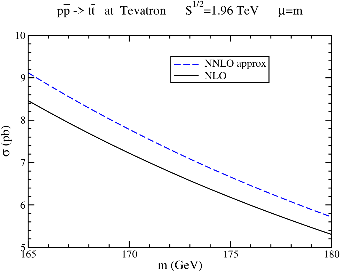
In Fig. 1 we plot the cross section for top-antitop production in proton-antiproton collisions at the Tevatron over a top quark mass range GeV at a factorization and renormalization scale . The exact NLO and the approximate NNLO cross sections are shown. The enhancement from the NNLO soft-gluon corrections is 7.8%. Here we have used the MSTW2008 NNLO parton distibution functions (pdf) [37]. We will use these pdf for our calculations throughout this paper except where noted otherwise.
| NNLO approx cross section (pb) | |||
|---|---|---|---|
| (GeV) | Tevatron | LHC 7 TeV | LHC 14 TeV |
| 170 | 7.78 | 179 | 998 |
| 171 | 7.54 | 173 | 972 |
| 172 | 7.31 | 168 | 946 |
| 173 | 7.08 | 163 | 920 |
| 174 | 6.87 | 158 | 896 |
| 175 | 6.66 | 154 | 873 |
Table 1 lists the values for the NNLO approximate cross section at the Tevatron for top quark masses between 170 GeV and 175 GeV. There are two kinds of theoretical uncertainties associated with the calculation: dependence on the factorization/renormalization scale, and uncertainties from the parton densities.

The scale dependence of the cross section for GeV is plotted in Fig. 2 over a range of two orders of magnitude, . It is clear that at leading order (LO) the cross section is strongly dependent on the choice of scale, varying by a factor of 5.45 between maximum and minimum values in the range shown. The NLO corrections significantly stabilize the LO variation: the NLO cross section varies by a factor of 1.61. The NNLO soft-gluon corrections further reduce the scale dependence: the NNLO approximate cross section varies by a factor of only 1.18. The improvement provided by the NNLO corrections is even more impressive if one considers only the variation as traditionally used to estimate errors. For this range the LO cross section varies by a factor of 1.85, the NLO cross section by 1.16, while the NNLO approximate cross section by a factor of only 1.034.
For a top quark mass of 173 GeV, the NLO cross section is pb and the NNLO approximate cross section is
| (3.1) |
Here the first uncertainty is from scale variation over and the second is from the MSTW2008 NNLO pdf errors at 90% C.L. (to be conservative, we do not use the smaller 68% C.L. pdf errors). At NLO the scale uncertainty is bigger than that from the pdf, but at NNLO the scale uncertainty is much smaller than the pdf one. In fact the scale uncertainty at NNLO is about four times smaller than that at NLO, again highlighting the dramatic reduction of scale dependence provided by the higher-order corrections. Adding the scale and pdf errors in quadrature, the NNLO approximate result is pb, i.e. we have a 5.1% total uncertainty, which is to be contrasted with a much larger (+6.6% -10.7%) total error (in quadrature) at NLO.

One can also study the dependence of the cross section separately on the factorization scale and the renormalization scale. This can be important because in some cases setting equal to may give a smaller uncertainty than from varying the scales independently. In Fig. 3 we plot the scale dependence of the cross section for GeV in three different ways at NLO (top plot) and approximate NNLO (bottom plot). The first way is to set and vary this common scale, exactly as we did in Fig. 2. The second way is to vary the factorization scale while keeping the renormalization scale fixed at . The third way is to vary while keeping . It is clear from the top plot that varying and independenty over the range and does not give a wider range of cross section values than varying the common scale . In fact as can be seen from the figure this holds true for a very wide range of scale variation. We also note that setting and or setting and still gives a smaller variation than varying the common scale between and . Therefore the NLO theoretical uncertainty that we provided above from scale variation is not increased by separately varying and . For the approximate NNLO cross section in the bottom plot of Fig. 3 we see that the variation with and affects the upper uncertainty (which was stated before as ) and this new upper uncertainty is . However the lower uncertainty () is unaffected. So the result for the approximate NNLO cross section for GeV with the scale uncertainy from independent and variation can be written as pb. Finally, we note that not only is the scale variation with greatly reduced in going from NLO to approximate NNLO but so is the separate variation and the separate variation.
The MSTW2008 parton densities are the only ones available at NNLO and so we use them for our best predictions. It is interesting nevertheless to see if the results change significantly using the new CT10 pdf [38], which are at NLO, and the pdf errors associated with them. Using CT10 pdf we find a NLO cross section for GeV of pb, and an approximate NNLO cross section of pb, where the first uncertainty is from scale variation (with and independently varied) and the second is from the pdf errors. We thus find both a larger cross section and a larger uncertainty with CT10 pdf than with MSTW2008 NNLO pdf.
3.2 Top quark distribution at the Tevatron
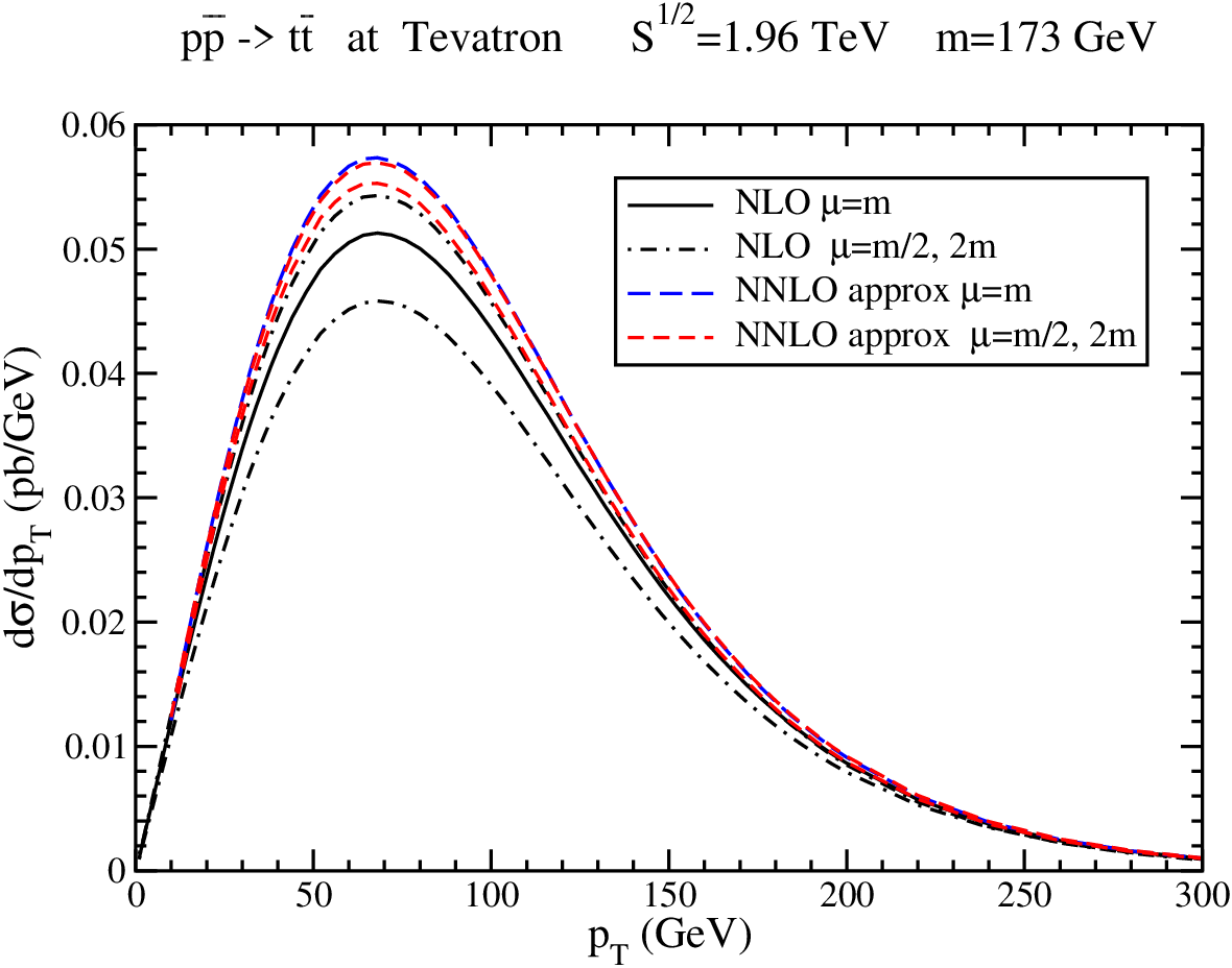
The top quark transverse momentum distribution at the Tevatron with GeV is plotted in Figs. 4 and 5 using the MSTW2008 NNLO pdf. Fig. 4 shows the differential distribution over a range GeV. Both NLO and NNLO approximate results are shown for three different scale choices, , , and . The integrated distribution gives the same result for the total cross section as found in the previous subsection, which provides a good consistency check of the calculation. The scale variation of the distribution at NNLO is again significantly smaller than at NLO. The NNLO soft-gluon corrections enhance the NLO result but the shape is similar.
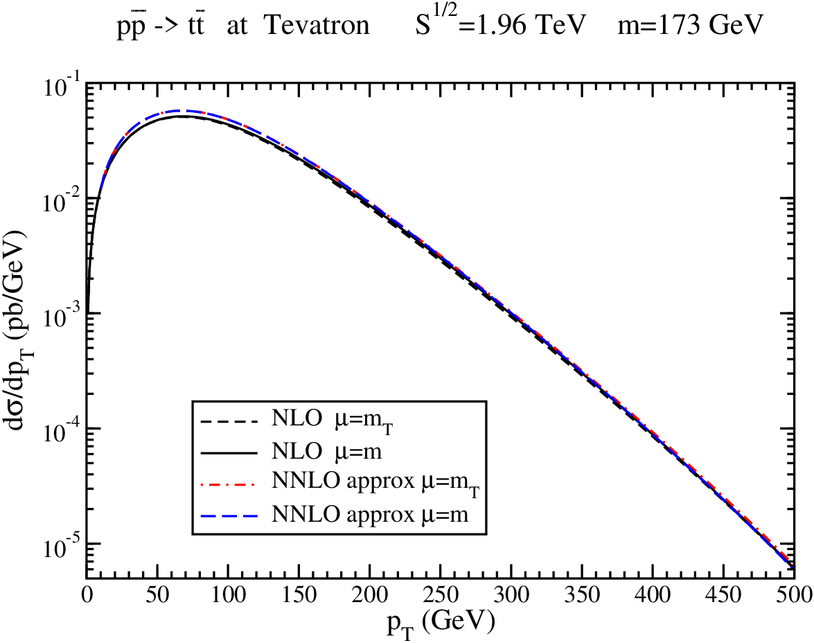
Figure 5 presents the top quark distribution in a logarithmic plot that makes it easier to see at high values. Results are now shown up to a of 500 GeV. In Fig. 4 the central value for the scale was taken to be as for the total cross section, and the scale variation was around that central value. Another possible scale choice for the top quark distribution is the transverse mass , defined by . In Fig. 5 we show our NLO and approximate NNLO results for both and . We find that the choice of scale, versus , makes very little difference even for high of 500 GeV - the curves are practically indistinguishable.
Joint threshold and recoil resummation for the distribution (at NLL accuracy only) has been studied in [39]. The effect of recoil is entirely negligible except at extremely high (800 GeV and above) so we do not consider it further.
4 Top cross section and distribution at the LHC
We continue with a detailed phenomenological study of top quark production in proton-proton collisions at the LHC. We present results for the current LHC energy of 7 TeV and the future (design) energy of 14 TeV, and also a few results at 10 TeV.
4.1 cross section at the LHC

In Fig. 6 we plot the NLO and approximate NNLO cross section for top-antitop production at the LHC at 7 TeV energy over a top quark mass range GeV at a factorization and renormalization scale using the MSTW2008 NNLO pdf. The enhancement from the NNLO soft-gluon corrections is 7.6%. Table 1 lists the values for the NNLO approximate cross section at the LHC at an enery of 7 TeV for top quark masses between 170 GeV and 175 GeV.

The scale dependence of the cross section for GeV is plotted in Fig. 7 over a range of two orders of magnitude, . Again, at LO the cross section is strongly dependent on the choice of scale, varying by a factor of 4.64 between maximum and minimum values in the range shown. The NLO corrections stabilize the LO variation: the NLO cross section varies by a factor of 1.85. The NNLO soft-gluon corrections further reduce the scale dependence: the NNLO approximate cross section varies by a factor of 1.43. The improvement from the NNLO corrections is again more impressive if one considers only the traditional variation . For this range the LO cross section varies by a factor of 1.75, the NLO cross section by 1.27, while the NNLO approximate cross section by a factor of only 1.08.
For a top quark mass of 173 GeV, the NLO cross section is pb and the NNLO approximate cross section is
| (4.1) |
where the first uncertainty is from scale variation over and the second is from the MSTW2008 NNLO pdf errors at 90% C.L. At NLO the scale uncertainty is about twice as big as the pdf one, but at NNLO it is significantly smaller. The scale uncertainty at NNLO is about three times smaller than that at NLO. Adding the scale and pdf errors in quadrature the NNLO approximate result is pb, i.e. we have a +7.0% -6.3% total uncertainty, which is to be contrasted with a much larger (+11.8% -13.8%) total error at NLO.

We also study the dependence of the cross section separately on the factorization scale and the renormalization scale. In Fig. 8 we plot the scale dependence of the cross section in three different ways at NLO (top plot) and approximate NNLO (bottom plot). The first way is to set and vary this common scale, as we did in Fig. 7. The second way is to vary while keeping , and the third way is to vary while keeping . From the top plot we see that varying and independenty over the range and does not give a wider range of cross section values than varying the common scale , and this actually holds true for nearly the entire wide range of scale variation shown in the plot. We also find that setting and or setting and still gives a smaller variation than varying the common scale between and . Therefore the NLO theoretical uncertainty from scale variation provided previously is not increased by separately varying and . For the approximate NNLO cross section in the bottom plot of Fig. 8 we also see that the independent variation of and does not affect the uncertainty that we wrote previously. Finally, we note that the separate variation and variation are reduced when going from NLO to approximate NNLO.
Again we can check if the results change significantly using the CT10 pdf, which are at NLO. Using CT10 pdf we find a NLO cross section at GeV of pb, and an approximate NNLO cross section of pb, so the results are very similar to those with MSTW2008 NNLO pdf.

For reference, the cross section at a possible future LHC energy of 10 TeV is plotted in Fig. 9 using the MSTW2008 NNLO pdf. For a top quark mass of 173 GeV, we find a NLO cross section of pb, while at NNLO
| (4.2) |

The cross section for the design LHC energy of 14 TeV is plotted in Fig. 10 using the MSTW2008 NNLO pdf. The enhancement from the NNLO soft-gluon corrections is 8.0%. Table 1 lists the values for the NNLO approximate cross section at 14 TeV LHC energy for top quark masses between 170 GeV and 175 GeV. The NLO cross section for a top quark mass of 173 GeV is pb and the approximate NNLO cross section is
| (4.3) |
Again we observe a significant decrease in scale dependence at NNLO relative to NLO, and also note that separate variation of and does not increase the uncertainty. The pdf uncertainties at this high energy are much smaller than the scale variation at NLO, and somewhat relatively smaller at NNLO. Adding the scale and pdf errors in quadrature the NNLO approximate result is pb, i.e. we have a +6.5% -5.7% total uncertainty, which is to be contrasted with a much larger (+11.2% -11.6%) total error at NLO.
4.2 Top quark distribution at the LHC

The transverse momentum distribution of the top quark with GeV at the LHC at 7 TeV energy is plotted in Figs. 11 and 12 using the MSTW2008 NNLO pdf. Fig. 11 shows NLO and approximate NNLO results for the differential distribution over a range GeV for three different scale choices, , , and . The scale variation of the distribution at NNLO is much smaller than that at NLO.

Figure 12 presents the results for in a logarithmic plot for high values up to 1000 GeV, using both and , where again is the transverse mass. At very high the NNLO approximate corrections become increasingly more significant and begin to change the shape of the distribution relative to NLO. This is not unexpected since the soft-gluon corrections are large near partonic threshold, which is dominant at high . The change of shape is more pronounced with the choice than it is with .

The distribution of the top quark with GeV at the LHC at 14 TeV energy is plotted in Figs. 13 and 14. Fig. 13 shows NLO and approximate NNLO results over a range GeV for three different scale choices, , , and . Again, the scale variation of the distribution at NNLO is much smaller than that at NLO.

Figure 14 presents the results for in a logarithmic plot for high values up to 1500 GeV, using and . The NNLO soft-gluon corrections provide a significant enhancement and change the shape of the NLO distribution at very high . Again, the change in shape is larger with the choice than it is with .
5 Comparison with other approaches and Conclusions
In this paper we have resummed the soft-gluon logarithms in top quark production to NNLL accuracy. This work directly extends the earlier NLL resummation in Ref. [15] and the further work in [33, 34] and later in [13, 14]. To achieve NNLL (NLL) accuracy, it is necessary to derive the soft anomalous dimension matrix at two (one) loops for each partonic process. At NLL and NNLL the color structure of the hard scattering enters the resummation in a non-trivial way. The soft anomalous dimension matrices are explicitly dependent on the kinematical variables , , , and the resummation involves these quantities and logarithms of , where measures distance from partonic threshold. Thus this is a fully differential calculation and the formalism in this paper has been used to calculate not only total cross sections but also differential cross sections, such as transverse momentum distributions. Approximate NNLO differential cross sections are extracted from the resummation (higher-order contributions beyond NNLO are small, see e.g. Ref. [35]). The NNLO expansion avoids the need for prescriptions to deal with Landau-pole divergences in the resummation, and we prefer to take this approach since the numerical discrepancies between different prescriptions are larger than the corrections beyond NNLO (see e.g. discussion in [33, 14]).
There also exist formalisms of resummation and finite-order expansions for the total cross section only [40] that are calculationally simpler, and only involve the variable . Logarithms of have been resummed at NLL in [40, 41] and at (partial) NNLL in [42] (Ref. [42] made an incorrect assumption about the two-loop terms which, as later understood, is not valid). This approach does not, however, involve the exact differential kinematics and hence numerical deviations from the exact kinematics-sensitive result may appear. Furthermore this approach is inapplicable to or other differential distributions, so it is limited in scope. For further discussion of the differences see also Ref. [14] and [30]. More recently, complete NNLL results in logarithms of have appeared in Ref. [25] using soft-collinear and non-relativistic effective theory, and in Ref. [26] using resummation in moment space. Threshold expansions to NNLO for the total cross section from this resummation have recently appeared in [43, 44]. Again, all these results are for total cross sections only, based on expansions in . It is important to note that the terminology “NLL” and “NNLL” means different things in the approaches of Refs. [25, 26, 40, 41, 42, 43, 44] than it does in the differential-level formalism of Refs. [13, 14, 15, 33, 34] and of this paper because different types of logarithms are resummed.
Another differential-level formalism that has recently appeared [30, 45] is based on soft-collinear effective theory and heavy-quark effective theory. While the resummation in [13, 14, 15, 33, 34] and this paper is done in moment space, in [30] it is performed in momentum space. The total cross section and invariant mass distribution at NNLL have been presented in [30]. The total cross section results in [30] are quite different from those in this paper. One major reason for the difference is the different choice of kinematics, as we describe below.
In Refs. [33, 34, 13, 14] (based on the formalism of [15]) results were provided in both single-particle-inclusive (1PI) and pair-invariant-mass (PIM) kinematics. The kinematics ambiguity was studied in detail in [34] and found to be an important source of uncertainty. In 1PI kinematics the soft-gluon logarithms are of the form and the soft-gluon corrections to the double differential cross section, , are calculated. In PIM kinematics, the soft logarithms are of the form with , and near threshold, where is the pair mass squared. In PIM kinematics, the soft gluon corrections to the double differential cross section, , where is the scattering angle in the partonic center-of-mass frame, are calculated. The cross section in PIM kinematics was found to be smaller than the 1PI result. The results in Refs. [33, 34] were based on NLL resummation and were later improved by adding subleading terms [13, 14]. The kinematics ambiguity was thus reduced in [13, 14]. Still it was shown in [13] that the PIM kinematics gives large negative results at NNLO for the channel at LHC energies (for production at the LHC, the channel is by far dominant over the channel). These negative corrections are deemed unphysical since already at NLO the PIM approximation for the corrections does not reproduce well the exact NLO result while the 1PI result is a much better approximation (detailed graphs for the partonic scaling functions in 1PI and PIM kinematics were shown in [34] and also [13]). In the present paper we have thus used 1PI kinematics. In contrast, Ref. [30] uses a modified PIM kinematics. Although the modified PIM kinematics of Ref. [30] produces less negative results than PIM in [34] and [13], the overall NNLO contribution in modified PIM is still negative. This explains why both the NNLL resummed cross section and the NNLO approximate cross section with modified PIM in [30] is less than the NLO cross section at for both Tevatron and LHC energies. This is in sharp contrast to the 1PI results here and in all our previous calculations (at both NLL and NNLL accuracy) where the NNLO soft-gluon corrections are found to provide a positive enhancement of the NLO cross section. The 1PI kinematics provides an excellent approximation as evidenced by the fact that the NLO approximate 1PI corrections from the expansion of the resummed cross section account for well over 98% (up to 99.8%) of the exact NLO corrections in the channel (with ) at both Tevatron and LHC energies. This is a far better agreement than can be attained with PIM or modified PIM kinematics. We thus remain of the opinion that the results in [30] do not accurately reflect the true contribution of soft-gluon corrections.
It is also interesting to compare the results in this paper with our previous results in [13, 14]. Although NNLL resummation requires calculation of the two-loop soft anomalous dimension matrices as presented in this paper, it was argued in [13, 14] that the numerical contribution of this matrix at two loops to the cross section is expected to be small. In [13, 14] many of the terms beyond NLL were already included in the calculation and it was argued based on the study of the scaling functions in 1PI and PIM kinematics that these additional subleading terms were relatively dominant. Now that the full two-loop NNLL terms are known it is important to revisit the validity of this argument. We find that indeed the new two-loop terms from the soft anomalous dimension matrices contribute very little to the total cross section, and hence the argument was valid and the results in [13, 14] were robust. For example, using the MSTW2008 NNLO pdf [37] the calculation at the accuracy of Ref. [14] for the top quark cross section at the LHC at 7 TeV gives 165 pb, while in this paper we find 163 pb based on NNLL resummation. The difference between the two numbers is very small compared with the overall theoretical uncertainty. Any differences in the numbers provided in [13, 14], and the present work are overwhelmingly due to the use of different pdf and only to a rather small extent due to the different theoretical accuracy.
To conclude, we have shown in this paper that the top quark cross section and transverse momentum distribution receive significant enhancements from soft-gluon corrections at NNLO. These corrections have been resummed at NNLL accuracy by calculating the two-loop soft anomalous dimension matrices for the partonic processes. Approximate NNLO total and differential cross sections have been derived from the NNLL resummed result. The NNLO soft-gluon corrections enhance the total cross section and the distribution and greatly reduce the theoretical uncertainty from scale variation. The pdf uncertainty of the cross section has also been presented. Our NNLL resummation formalism can be used to calculate other differential distributions of interest, such as the top quark rapidity distribution. This will be a topic of future work.
Acknowledgements
This work was supported by the National Science Foundation under Grant No. PHY 0855421.
References
- [1]
CDF Collaboration, F. Abe et al., Phys. Rev. Lett. 74,
2626 (1995) [hep-ex/9503002];
D0 Collaboration, S. Abachi et al., Phys. Rev. Lett. 74, 2632 (1995) [hep-ex/9503003]. - [2] CDF Collaboration, T. Aaltonen et al., Phys. Rev. D 79, 052007 (2009) [arXiv:0901.4142 [hep-ex]]; Phys. Rev. D 79, 112007 (2009) [arXiv:0903.5263 [hep-ex]]; Phys. Rev. D 81, 052011 (2010) [arXiv:1002.0365 [hep-ex]]; Phys. Rev. D 82, 052002 (2010) [arXiv:1002.2919 [hep-ex]]; Phys. Rev. D 81, 092002 (2010) [arXiv:1002.3783 [hep-ex]]; arXiv:1007.4423 [hep-ex].
- [3] D0 Collaboration, V.M. Abazov et al., Phys. Rev. Lett. 100, 192004 (2008) [arXiv:0803.2779 [hep-ex]]; Phys. Lett. B 679, 177 (2009) [arXiv:0901.2137 [hep-ex]]; Phys. Rev. D 80, 071102 (2009) [arXiv:0903.5525 [hep-ex]]; Phys. Rev. D 82, 032002 (2010) [arXiv:0911.4286 [hep-ex]]; Phys. Rev. D 82, 071102 (2010) [arXiv:1008.4284 [hep-ex]].
- [4] CDF Collaboration, A.A. Affolder et al., Phys. Rev. Lett. 87, 102001 (2001); CDF II Collaboration, CDF Note 10234; D0 Collaboration, V.M. Abazov et al., Phys. Lett. B 693, 515 (2010) [arXiv:1001.1900 [hep-ex]].
- [5] D0 Collaboration, V.M. Abazov et al., Phys. Rev. Lett. 103, 092001 (2009) [arXiv:0903.0850 [hep-ex]]; Phys. Lett. B 682, 363 (2010) [arXiv:0907.4259 [hep-ex]]; Phys. Lett. B 690, 5 (2010) [arXiv:0912.1066 [hep-ex]].
- [6] CDF Collaboration, T. Aaltonen et al., Phys. Rev. Lett. 103, 092002 (2009) [arXiv:0903.0885 [hep-ex]]; Phys. Rev. D 81, 072003 (2010) [arXiv:1001.4577 [hep-ex]]; arXiv:1004.1181 [hep-ex].
- [7] Tevatron Electroweak Working Group, arXiv:0808.1089 [hep-ex]; arXiv:0903.2503 [hep-ex]; arXiv:1007.3178 [hep-ex].
- [8] R. Kehoe, M. Narain, and A. Kumar, Int. J. Mod. Phys. A 23, 353 (2008) [arXiv:0712.2733 [hep-ex]]; E.W. Varnes, Int. J. Mod. Phys. A 23, 4421 (2008) [arXiv:0810.3652 [hep-ex]]; M.-A. Pleier, Int. J. Mod. Phys. A 24, 2899 (2009) [arXiv:0810.5226 [hep-ex]]; P. de Jong, arXiv:0902.4798 [hep-ex]; J.R. Incandela, A. Quadt, W. Wagner, and D. Wicke, Prog. Part. Nucl. Phys. 63, 239 (2009) [arXiv:0904.2499 [hep-ex]]; A.P. Heinson, Mod. Phys. Lett. A 25, 309 (2010) [arXiv:1002.4167 [hep-ex]]; F. Fiedler, arXiv:1003.0521 [hep-ex]; W. Wagner, Mod. Phys. Lett. A 25, 1297 (2010) [arXiv:1003.4359 [hep-ex]]; C. Schwanenberger, PoS (EPS-HEP 2009) 017 [arXiv:1004.5268 [hep-ex]]; B. Stelzer, arXiv:1004.5368 [hep-ex].
- [9] T. Han, Int. J. Mod. Phys. A 23, 4107 (2008) [arXiv:0804.3178 [hep-ph]]; W. Bernreuther, J. Phys. G 35, 083001 (2008) [arXiv:0805.1333 [hep-ph]]; E. Laenen, arXiv:0809.3158 [hep-ph]; D. Wackeroth, arXiv:0810.4176 [hep-ph]; R. Bonciani and A. Ferroglia, PoS (EPS-HEP 2009) 350 [arXiv:0909.2980 [hep-ph]]; W. Bernreuther, arXiv:1008.3819 [hep-ph].
- [10] P. Nason, S. Dawson, and R.K. Ellis, Nucl. Phys. B 303, 607 (1988); Nucl. Phys. 327, 49 (1989); (E) B 335, 260 (1990).
- [11]
W. Beenakker, H. Kuijf, W.L. van Neerven, and J. Smith,
Phys. Rev. D 40, 54 (1989);
W. Beenakker, W.L. van Neerven, R. Meng, G.A. Schuler, and J. Smith, Nucl. Phys. B 351, 507 (1991). - [12] W. Beenakker, A. Denner, W. Hollik, R. Mertig, T. Sack, and D. Wackeroth, Nucl. Phys. B 411, 343 (1994); C. Kao, G.A. Ladinsky, and C.P. Yuan, Int. J. Mod. Phys. A 12, 1341 (1997); W. Bernreuther, M. Fuecker, and Z.G. Si, Phys. Lett. B 633, 54 (2006) [hep-ph/0508091]; Phys. Rev. D 74, 113005 (2006) [hep-ph/0610334]; J.H. Kuhn, A. Scharf, and P. Uwer, Eur. Phys. J. C 45, 139 (2006) [hep-ph/0508092]; Eur. Phys. J. C 51, 37 (2007) [hep-ph/0610335]; S. Moretti, M.R. Nolten, and D.A. Ross, Phys. Lett. B 639, 513 (2006) [hep-ph/0603083]; (E) B 660, 607 (2008); W. Hollik and M. Kollar, Phys. Rev. D 77, 014008 (2008) [arXiv:0708.1697 [hep-ph]]; W. Bernreuther and Z.G. Si, Nucl. Phys. B 837, 90 (2010) [arXiv:1003.3926 [hep-ph]].
- [13] N. Kidonakis and R. Vogt, Phys. Rev. D 68, 114014 (2003) [hep-ph/0308222].
- [14] N. Kidonakis and R. Vogt, Phys. Rev. D 78, 074005 (2008) [arXiv:0805.3844 [hep-ph]].
- [15] N. Kidonakis and G. Sterman, Phys. Lett. B 387, 867 (1996); Nucl. Phys. B 505, 321 (1997) [hep-ph/9705234].
- [16] S.M. Aybat, L.J. Dixon, and G. Sterman, Phys. Rev. Lett. 97, 072001 (2006) [hep-ph/0606254]; Phys. Rev. D 74, 074004 (2006) [hep-ph/0607309].
- [17] L.J. Dixon, L. Magnea, and G. Sterman, JHEP 08, 022 (2008) [arXiv:0805.3515 [hep-ph]].
- [18] T. Becher and M. Neubert, Phys. Rev. Lett. 102, 162001 (2009) [arXiv:0901.0722 [hep-ph]]; JHEP 06, 081 (2009) [arXiv:0903.1126 [hep-ph]].
- [19] E. Gardi and L. Magnea, JHEP 03, 079 (2009) [arXiv:0901.1091 [hep-ph]]; Nuovo Cim. C 32, 137 (2009) [arXiv:0908.3273 [hep-ph]].
- [20] L.J. Dixon, Phys. Rev. D 79, 091501 (2009) [arXiv:0901.3414 [hep-ph]].
- [21] L.J. Dixon, E. Gardi, and L. Magnea, JHEP 02, 081 (2010) [arXiv:0910.3653 [hep-ph]]; PoS (RADCOR2009) 007 [arXiv:1001.4709 [hep-ph]].
- [22] N. Kidonakis, Phys. Rev. Lett. 102, 232003 (2009) [arXiv:0903.2561 [hep-ph]]; in DPF 2009, eConf C090726 [arXiv:0910.0473 [hep-ph]].
- [23] A. Mitov, G. Sterman, and I. Sung, Phys. Rev. D 79, 094015 (2009) [arXiv:0903.3241 [hep-ph]].
- [24] T. Becher and M. Neubert, Phys. Rev. D 79, 125004 (2009) [arXiv:0904.1021 [hep-ph]].
- [25] M. Beneke, P. Falgari, and C. Schwinn, Nucl. Phys. B 828, 69 (2010) [arXiv:0907.1443 [hep-ph]]; PoS (EPS-HEP 2009) 319 [arXiv:0909.3488 [hep-ph]]; PoS (RADCOR2009) 011 [arXiv:1001.4621 [hep-ph]].
- [26] M. Czakon, A. Mitov, and G. Sterman, Phys. Rev. D 80, 074017 (2009) [arXiv:0907.1790 [hep-ph]].
- [27] A. Ferroglia, M. Neubert, B.D. Pecjak, and L.L. Yang, Phys. Rev. Lett. 103, 201601 (2009) [arXiv:0907.4791 [hep-ph]]; JHEP 11, 062 (2009) [arXiv:0908.3676 [hep-ph]].
- [28] N. Kidonakis, Phys. Rev. D 81, 054028 (2010) [arXiv:1001.5034 [hep-ph]].
- [29] N. Kidonakis, Phys. Rev. D 82, 054018 (2010) [arXiv:1005.4451 [hep-ph]].
- [30] V. Ahrens, A. Ferroglia, M. Neubert, B.D. Pecjak, and L.L. Yang, JHEP 09, 097 (2010) [arXiv:1003.5827 [hep-ph]].
- [31] A. Mitov, G. Sterman, and I. Sung, Phys. Rev. D 82, 034020 (2010) [arXiv:1005.4646 [hep-ph]].
- [32] M. Beneke, P. Falgari, and C. Schwinn, Nucl. Phys. B 842, 414 (2011) [arXiv:1007.5414 [hep-ph]].
- [33] N. Kidonakis, Phys. Rev. D 64, 014009 (2001) [hep-ph/0010002].
- [34] N. Kidonakis, E. Laenen, S. Moch, and R. Vogt, Phys. Rev. D 64, 114001 (2001) [hep-ph/0105041].
- [35] N. Kidonakis, Phys. Rev. D 73, 034001 (2006) [hep-ph/0509079].
- [36]
G.P. Korchemsky and A.V. Radyushkin, Phys. Lett. B 171, 459 (1986);
Nucl. Phys. B 283, 342 (1987). - [37] A.D. Martin, W.J. Stirling, R.S. Thorne, and G. Watt, Eur. Phys. J. C 63, 189 (2009) [arXiv:0901.0002 [hep-ph]].
- [38] H.-L. Lai, M. Guzzi, J. Huston, Z. Li, P.M. Nadolsky, J. Pumplin, and C.-P. Yuan, Phys. Rev. D 82, 074024 (2010) [arXiv:1007.2241 [hep-ph]].
- [39] A. Banfi and E. Laenen, Phys. Rev. D 71, 034003 (2005) [hep-ph/0411241].
- [40] R. Bonciani, S. Catani, M.L. Mangano, and P. Nason, Nucl. Phys. B 529, 424 (1998) [hep-ph/9801375]; (E) B 803, 234 (2008).
- [41] M. Cacciari, S. Frixione, M.L. Mangano, P. Nason, and G. Ridolfi, JHEP 09, 127 (2008) [arXiv:0804.2800 [hep-ph]].
- [42] S. Moch and P. Uwer, Phys. Rev. D 78, 034003 (2008) [arXiv:0804.1476 [hep-ph]].
- [43] M. Beneke, M. Czakon, P. Falgari, A. Mitov, and C. Schwinn, Phys. Lett. B 690, 483 (2010) [arXiv:0911.5166 [hep-ph]].
- [44] M. Beneke, P. Falgari, S. Klein, and C. Schwinn, arXiv:1009.4011 [hep-ph].
- [45] V. Ahrens, A. Ferroglia, M. Neubert, B.D. Pecjak, and L.L. Yang, Phys. Lett. B 687, 331 (2010) [arXiv:0912.3375 [hep-ph]].