Effective dynamics for $N$-solitons of the Gross-Pitaevskii equation

In many situations a wave moving in a slowly varying field, that is, a field described by a potential whose derivatives are much smaller than the oscillations/width of the wave, can be described using classical dynamics. This is the basis of the semiclassical/short wave approximation, perhaps best known in the case of the linear Schrödinger equation,

(1.1)

$$ih\partial_{t}u=-\frac{1}{2}h^{2}\partial_{x}^{2}u+V(x)u\,,$$

where $V$ is an infinitely differentiable potential. A typical result concerns a propagation of a coherent state

$$u(x,0)=\exp\left(\frac{i}{h}\left((x-x_{0})\xi_{0}+i(x-x_{0})^{2}/2\right)\right)\,,$$

maximally concentrated near the point $(x_{0},\xi_{0})$ in the position-momentum space. In that case,

(1.2)

$$u(x,t)=a_{0}(x,t)\exp\left(\frac{i}{h}\varphi(x,t)\right)+{\mathcal{O}}(h^{\frac{1}{2}})\,,\ \ 0<t<T(h)\,,$$

where $\mathop{\rm Im}\nolimits\partial_{x}^{2}\varphi>0$, $\mathop{\rm Im}\nolimits\varphi\geq 0$, and

$$\mathop{\rm Im}\nolimits\varphi(x,t)=0\ \Rightarrow\ x=x(t)\,,\ \ \partial_{x}\varphi(x,t)=\xi(t)\,,$$

where $(x(t),\xi(t))$ satisfy Newton’s equations:

(1.3)

$$x^{\prime}(t)=\xi(t)\,,\ \ \xi^{\prime}(t)=-V^{\prime}(x)\,,\ \ x(0)=x_{0}\,,\ \ \xi(0)=\xi_{0}\,.$$

The time of the validity of (1.2), $T(h)$, depends on the properties of the flow (1.3), and in general it is limited by the Ehrenfest time,

(1.4)

$$T(h)\sim\ \log\left(\frac{1}{h}\right)\,,$$

see [1] for a recent discussion on the case of one dimension.

The approximation (1.2) means that the solution is concentrated for logarithmically long times on classical trajectories. The phase $\varphi$ and the amplitude $a_{0}$ can be described very precisely and $a_{0}$ can be refined to give an asymptotic expansion – see [6] for an early mathematical treatment and [13] for more recent developments and references.

In this paper we consider the Gross-Pitaevski equation, which is the cubic non-linear Schrödinger equation with a potential:

(1.5)

$$ih\partial_{t}u=-\frac{1}{2}h^{2}\partial_{x}^{2}u-u|u|^{2}+V(x)u\,.$$

It provides a mean field approximation for the evolution of Bose-Einstein condensate in an external field given by the potential $V(x)$ – see the monograph [12] and references given there. Questions about propagation of localized states are also natural in the setting of (1.5) and have been much studied. One direction is described in a recent monograph [2].

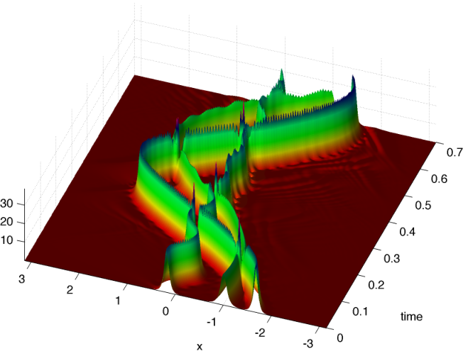
In this note we present a numerical study of multiple soliton propagation for (1.5) and show that it can be described very accurately using a natural effective dynamics – see Figure 1. That effective dynamics is based on mathematical results of Holmer-Zworski [8] and Holmer-Perelman-Zworski [7] and we refer to those papers for pointers to earlier mathematical works on that subject.

Following the convention of earlier papers – see Fröhlich et al [4] – we rescale equation (1.5) so that the parameter $h$ is in the potential which is now slowly varying:

(1.6)

$$i\partial_{t}u=-\frac{1}{2}\partial_{x}^{2}u-u|u|^{2}+V(x)u\,,\qquad V(x)=W(hx)\,.$$

For $V\equiv 0$ this equation is completely integrable – see for instance [3]. One of the most striking consequences of that is the existence of exact $N$-soliton solutions:

$$\displaystyle\begin{gathered}u(x,t)=q_{N}(x,a+tv,v,\theta+\frac{t}{2}(\mu^{2}+v^{2}),\mu)\,,\\ a,v\in\mathbb{R}^{N}\,,\ \ \theta\in(\mathbb{R}/2\pi\mathbb{Z})^{N}\,,\ \ \mu\in\mathbb{R}^{N}_{+}\,,\end{gathered}$$

where the construction of $q_{N}=q_{N}(x,a,v,\theta,\mu)$ will be recalled in §2.

When $V\not\equiv 0$ and

$$u(x,0)=q_{N}(x,a,v,\theta,\mu)\,,$$

the exact dynamics (1) is replaced by

$$\displaystyle\begin{gathered}u(x,t)=q_{N}(x,a(t),v(t),\theta(t),\mu(t))+{\mathcal{O}}(h^{2})\,,\end{gathered}$$

where the precise meaning of the error, and its optimality, will be described below. The parameters of the multisoliton approximation solve the system of ordinary differential equations:

$$\displaystyle\begin{gathered}\dot{v_{j}}=-\mu_{j}^{-1}(\partial_{a_{j}}V_{N}+v_{j}\partial_{\theta_{j}}V_{N})\,,\ \ \dot{a}_{j}=v_{j}+\mu_{j}^{-1}\partial_{v_{j}}V_{N}\,,\\ \dot{\mu}_{j}=\partial_{\theta_{j}}V_{N}\,,\ \ \dot{\theta}_{j}=v_{j}^{2}/2+\mu^{2}_{j}/2+\mu_{j}^{-1}v_{j}\partial_{v_{j}}V_{N}-\partial_{\mu_{j}}V_{N}\,,\end{gathered}$$

and where

$$V_{N}(a,v,\theta,\mu)\stackrel{{\scriptstyle\text{\tiny def}}}{{=}}\frac{1}{2}\int_{\mathbb{R}}V(x)|q_{N}(x,a,v,\theta,\mu)|^{2}\,dx\,.$$

Although somewhat complicated looking, the equations (1) have a natural interpretation in terms of Hamiltonian systems: they are the Hamilton-Jacobi equations for the full Hamiltonian of (1.6) restricted to the symplectic $4N$-dimensional manifold of $N$-solitons – see §3 for details. Of course when $V\equiv 0$ the solutions correspond to the exact solutions of (1). The mathematical results of [7], [8] suggest that the approximation (1) is valid up to a (rescaled) Ehrenfest time (1.4):

(1) holds for $0<t<C\log(1/h)/h$.

In other words, the equations (1) give the minimal exact effective dynamics valid up to the Ehrenfest time $\log(1/h)/h$, where $h$ is the parameter controlling the small variation of the potential, see (3.1). In this work, we show that the approximation errors ${\mathcal{O}}(h^{2})$ and the Ehrenfest time bound are sharp. See [11] for a survey of soliton dynamics under integrable systems that have been perturbed.

One motivation for this study is the experimental and theoretical investigation of soliton trains in Bose-Einstein condensates [14]. We show that the effective dynamics described in §3 is in qualitative agreement with the behaviour of the matter-wave soliton trains – see Figure 2.

The paper is organized as follows: in §2 we recall the construction of $N$-soliton solutions for $V\equiv 0$ and in §3, the Hamiltonian structure of the equation and the derivation of the effective equations of motion. In §4 we compare the effective dynamics to the behaviour of solutions to (1.6) and draw some quantitative conclusions. Specific potentials similar to those in [14] are then discussed in §5. We investigate effective dynamics for the mKdV equation in §6. Finally, in §7 we describe the numerical methods and compare to other possible approaches.

When $V\equiv 0$, we recover the nonlinear cubic one dimensional Schrödinger equation, which has $N$-soliton solutions with explicit formulas that we now recall – see [3] for a detailed presentation of this completely integrable equation.

We will construct functions $q_{N}(x)$ that depend on $4N$ parameters: positions, velocities, phases, and masses:

(2.1)

$$q_{N}(x)=q_{N}(x,a,v,\theta,\mu),\quad a,v,\theta\in\mathbb{R}^{N},\quad\mu\in(0,\infty)^{N}.$$

Put

(2.2)

$$\lambda_{j}=v_{j}+i\mu_{j}\,,\ \ \quad\gamma_{j}(x)=e^{i\lambda_{j}x}e^{i(\theta_{j}-v_{j}a_{j})}e^{\mu_{j}a_{j}}\,,$$

and define matrices

$$M(x)\in\mathbb{R}^{N\times N}\,,\ \ \ \ \ M_{1}(x)\in\mathbb{R}^{(N+1)\times(N+1)}\,,$$

by

(2.3)

$$M_{jk}(x)=\frac{1+\gamma_{j}(x)\bar{\gamma}_{k}(x)}{\lambda_{j}-\bar{\lambda}_{k}}\,,\ \ \ M_{1}=\left[\begin{array}[]{cc}M(x)&\gamma\\ &\\ \vec{1}&0\end{array}\right]$$

where

(2.4)

$$\gamma=\left[\gamma_{1},\cdots,\gamma_{N}\right]^{T},\quad\vec{1}=\left[1,\cdots,1\right]\in\mathbb{R}^{N}.$$

Finally,

(2.5)

$$q_{N}(x)\stackrel{{\scriptstyle\text{\tiny def}}}{{=}}\frac{\det M_{1}(x)}{\det M(x)}.$$

Remarkably, this gives a solution to (1.5) with $V\equiv 0$, the $N$-soliton solution:

(2.6)

$$u(x,t)=q_{N}(x,a+tv,v,\theta+\frac{t}{2}(\mu^{2}+v^{2}),\mu)\,.$$

As one can see from the formula, some restrictions on the parameters apply, see [3].

We consider potentials defined on $\mathbb{R}$ that are slowly varying in the sense that

(3.1)

$$V(x)=W(hx)$$

where $W(x)$ is $C^{2}$ in $x$, and

$$|\partial_{x}^{k}W(x)|\leq C(1+|x|)^{N}\,,k\leq 2\,.$$

where $C$ and $N$ are independent of $h$. This means that $h$ is the parameter controlling the slow variation of $V$.

To obtain an effective dynamics for the evolution we use the Hamiltonian structure of the equation. In the physics literature an approach using Lagrangians is more common – see for instance Goodman-Holmes-Weinstein [5] and Strecker et al [14]. In the mathematics treatments [4],[8],[7] the Hamiltonian approach was found easier to use, which we follow here.

The basic claim is that an approximate evolution of $q_{N}$ is obtained by restricting the Hamiltonian flow generated by the Gross-Pitaevskii equation to the manifold of $N$-solitons described in §2. The Hamiltonian associated with the Gross-Pitaevskii equation is

(3.2)

$$H_{V}(u)\stackrel{{\scriptstyle\text{\tiny def}}}{{=}}\frac{1}{4}\int(|\partial_{x}u|^{2}-|u|^{4})\,dx+\frac{1}{2}\int V|u|^{2}$$

with respect to the symplectic form

(3.3)

$$\omega(u,v)=\mbox{Im}\int u\bar{v}\,.$$

The manifold of solitons, $M_{N}$, is $4N$-dimensional and equipped with the restricted symplectic form given by the sum of forms for single solitons:

(3.4)

$$\omega_{M}\stackrel{{\scriptstyle\text{\tiny def}}}{{=}}\omega|_{M}=\sum_{j=1}^{N}(\mu_{j}dv_{j}\wedge da_{j}+v_{j}d\mu_{j}\wedge da_{j}+d\theta_{j}\wedge d\mu_{j})\,.$$

$H_{V}$ restricted to $M_{N}$ is

(3.5)

$$H_{N}\stackrel{{\scriptstyle\text{\tiny def}}}{{=}}H_{V}|_{M_{N}}(a,v,\theta,\mu)=\sum_{j=1}^{N}\left(\frac{\mu_{j}v_{j}^{2}}{2}-\frac{\mu_{j}^{3}}{6}\right)+V_{N}(a,v,\theta,\mu)\,,$$

(3.6)

$$\mbox{where}\quad V_{N}(a,v,\theta,\mu)\stackrel{{\scriptstyle\text{\tiny def}}}{{=}}\frac{1}{2}\int_{\mathbb{R}}V(x)|q_{N}(x,a,v,\theta,\mu)|^{2}\,dx\,.$$

The effective dynamics is given by the flow of the Hamilton vector field of $H_{N}$ on the manifold $M_{N}$. That vector field, $\Xi_{H_{N}}$, is defined using the symplectic form (3.4):

(3.7)

$$dH_{N}=\omega_{M}(\cdot,\Xi_{H_{N}})\,.$$

A computation based on this gives the following ordinary differential equation for the parameters $a,v,\theta$ and $\mu$, called the effective dynamics:

(3.8)

$$\begin{split}\dot{v}_{j}&=-\mu_{j}^{-1}\partial_{a_{j}}H_{N}-\mu_{j}^{-1}v_{j}\partial_{\theta_{j}}H_{N}=-\mu_{j}^{-1}(\partial_{a_{j}}V_{N}+v_{j}\partial_{\theta_{j}}V_{N})\,,\\ \dot{a}_{j}&=\mu_{j}^{-1}\partial_{v_{j}}H_{N}=v_{j}+\mu_{j}^{-1}\partial_{v_{j}}V_{N}\,,\\ \dot{\mu}_{j}&=\partial_{\theta_{j}}H_{N}=\partial_{\theta_{j}}V_{N}\,,\\ \dot{\theta}_{j}&-=\mu_{j}^{-1}v_{j}\partial_{v_{j}}H_{N}-\partial_{\mu_{j}}H_{N}=v_{j}^{2}/2+\mu^{2}_{j}/2+\mu_{j}^{-1}v_{j}\partial_{v_{J}}V_{N}-\partial_{\mu_{j}}V_{N}\,.\end{split}$$

We remark that one can scale the Gross-Pitaevskii equation (1.6) in the following way: Consider any function $u(x,t)$, scaling parameter $\alpha$, let $\tilde{x}=\alpha x\,,\tilde{t}=\alpha^{2}t$, and define the new function

(3.9)

$$\tilde{u}(\tilde{x},\tilde{t})\stackrel{{\scriptstyle\text{\tiny def}}}{{=}}\frac{1}{\alpha}u(x,t)\,.$$

Then if $u(x,t)$ satisfies (1.6) with the potential $V(x)$, $\tilde{u}(\tilde{x},\tilde{t})$ also satisfies (1.6) with the new potential

(3.10)

$$\tilde{V}(\tilde{x})=\frac{1}{\alpha^{2}}V\left(\frac{\tilde{x}}{\alpha}\right)\,.$$

This means that if we deal with a soliton of width comparable with $\alpha$, the potentials for which interesting dynamics should appear should have size approximately $\alpha^{-2}$ and the slowly varying factor replaced by $h/\alpha$.

The effective dynamics equations (3.8) scale similarly: if $\left(a(t),v(t),\theta(t),\mu(t)\right)$ satisfies (3.8) and we define $\tilde{x},\tilde{t},$ and $\tilde{V}$ as above, then $\left(\tilde{a}(\tilde{t}),\tilde{v}(\tilde{t}),\tilde{\theta}(\tilde{t}),\tilde{\mu}(\tilde{t})\right)$ also satisfies (3.8) with

(3.11)

$$\tilde{a}(\tilde{t})=\alpha a(t)\,,\quad\tilde{v}(\tilde{t})=\frac{v(t)}{\alpha}\,,\quad\tilde{\theta}(\tilde{t})=\theta(t)\,,\quad\tilde{\mu}(\tilde{t})=\frac{\mu(t)}{\alpha}\,.$$

The scalings (3.9) and (3.11) are related in the following way: if

$$u(x,t)=q_{N}(x,a(t),v(t),\theta(t),\mu(t))\,,$$

then

$$\tilde{u}(\tilde{x},\tilde{t})=q_{N}(\tilde{x},a(\tilde{t}),v(\tilde{t}),\theta(\tilde{t}),\mu(\tilde{t}))/\alpha=q_{N}(x,\tilde{a}(\tilde{t}),\tilde{v}(\tilde{t}),\tilde{\theta}(\tilde{t}),\tilde{\mu}(\tilde{t}))\,.$$

For given values $a_{0},v_{0},\theta_{0},\mu_{0}$ in $\mathbb{R}^{N}$, we consider the solution $u(\cdot,t)$ of (1.6) with initial data $q_{N}(\cdot,a_{0},v_{0},\theta_{0},\mu_{0})$ and the solutions $a(t),v(t),\theta(t),\mu(t)$ of the effective dynamics equations (3.8) with initial values $a_{0},v_{0},\theta_{0},\mu_{0}$. In the following discussions we will refer to $u(\cdot,t)$ as the exact solution and $q_{N}(\cdot,a(t),v(t),\theta(t),\mu(t))$ as the effective dynamics.

Holmer and Zworski [8] proved that in the case $N=1$,

(4.1)

$$\|u(\cdot,t)-q_{N}(\cdot,a(t),v(t),\theta(t),\mu(t))\|_{H^{1}}=Ch^{2-\delta}\,,\mbox{ for }t<\frac{\delta\log(1/h)}{Ch}\,,$$

where $\delta\in(0,1/2)$ can be chosen, and where $C$ depends only on the potential and initial velocity of the soliton, but not on $\delta$. The $H^{1}$ norm measures the size of the function and its spatial derivative in $L^{2}$:

$$\|v\|_{H^{1}}^{2}\stackrel{{\scriptstyle\rm{def}}}{{=}}\|v\|_{L^{2}}^{2}+\|\partial_{x}v\|_{L^{2}}^{2}\,,\qquad\|v\|_{L^{2}}^{2}\stackrel{{\scriptstyle\rm{def}}}{{=}}\int_{\mathbb{R}}|v(x)|^{2}dx\,.$$

This norm measures the energy of the solution.

The limiting time $\log(1/h)/h$ is the Ehrenfest time discussed int §1.

It is expected that this result also holds for $N>1$. This is suggested by [7], which proves the analagous theorem for the modified Korteweg-de Vries (mKdV) equations for case $N=1,2$, see §6 below. However, the methods of [7] do not fully apply to the case of the Gross-Pitaevsky equation (1.5). Also, even in the case of mKdV and $N=2$, multiple soliton interactions are not theoretically understood. All these considerations provided a strong motivation for this numerical study.

We note that for $N>1$, it was conjectured in [7] that the error bounds (4.1) will hold not only in the $H^{1}$ norm, but for the $H^{N}$ norm, which measures the the size of a function and its first $N$ derivatives, where $N$ is the number of solitons. This has been proven in the mKdV case with $N=2$ [7]. For our numerical experiments, we consider only the $H^{1}$ norm.

We present numerical simulations to show that the result (4.1) holds for $N>1$ in the following three sections: In §4.1 we choose initial data and two potentials that demonstrate the power and limitations of the effective dynamics equations, regardless of the number of solitons. Using the same initial data and one of the potentials from §4.1, in §4.2 we verify that the $\mathcal{O}(h^{2-\delta})$ error estimate in (4.1) holds as $h\to 0$ for a fixed time interval. We then turn to the $\log(1/h)/h$ timescale, or Ehrenfest timescale, in §4.3 to show that it is the appropriate timescale for which we can expect (4.1) to hold.

Strecker, Partridge, Truscott and Hulet [14] discovered that Bose-Einstein condensates form stable soliton trains while confined to one-dimensional motion. When set into motion in a suitably chosen optical trap, a Bose-Einstein condensate forms multiple soliton formations which exist for multiple oscillatory cycles without being destroyed by dispersion or diffraction. We can observe this same behavior numerically, using the effective dynamics equations. We choose a potential of the type described in [14]

$$V(x)=\left(\frac{x}{2}\right)^{6}$$

and set $N=4$, which was the most frequent case in their experiment. Strecker et al inferred that the repulsive behavior of the solitons indicated alternating phases. Their argument was based on considering a certain reduced Lagrangian.

In our numerical experiment we put $\bar{\theta}=(0,\pi,0,\pi)$ and then set the four solitons in motion with the same velocity near the center of the potential. Similar to [14], we observe bunching and spreading of the soliton train for several oscillations. See Figure 2.

The mKdV equation

(6.1)

$$\partial_{t}u=-\partial_{x}(\partial_{x}^{2}u+2u^{3})\,,$$

like the nonlinear Schrödinger equation, has soliton solutions and a Hamiltonian structure. Holmer, Perelman, and Zworski [7] derived effective dynamics equations for the mKdV equation with a slowly varying potential

(6.2)

$$\partial_{t}u=-\partial_{x}(\partial_{x}^{2}u-b(x,t)u+2u^{3}),\quad b(x,t)=b_{0}(hx,ht)$$

and proved a result analogous to the (4.1) for $N=1,2$: the $H^{N}$ error between the solution of (6.2) and its associated effective dynamics with $N$-soliton initial data is bounded by

(6.3)

$$Ch^{2}e^{Cht}\,,\ \ \ \ \ \text{ for }\ \ t<\frac{C}{h}\log\frac{1}{h},$$

Similarly to §4.2, we have conducted a numerical study verifying that the $H^{1}$ error is $\mathcal{O}(h^{2})$ as $h\to 0$ for multiple soliton initial conditions. See Figures 9 and 10.

We now describe the numerical methods we employ to compute the Gross-Pitaevskii PDE (1.6) and the ODE (3.8) arising from the effective dynamics. When comparing a solution of (1.6) with a solution of (3.8), we refine our numerical solutions until the error between sucessive refinements of solutions to the same equation is several orders of magnitude smaller than the error between solutions of the two equations.

Numerically solving the ODE arising from the effective dynamics (3.8) necessitates computing $q_{N}(x,a,v,\theta,\mu)$ and its derivatives with respect to the parameters $a,v,\theta$,and $\mu$ efficiently. For this we note that an equivalent definition of $q_{N}$ in (2.5)

(7.1)

$$q_{N}(x)=-\vec{1}M^{-1}\gamma\,,$$

where $\vec{1},M$, and $\gamma$ are as in (2.5). Since $iM$ is Hermitian, $M^{-1}\gamma$ can be efficiently computed using the Cholesky factorization. Differentiating $q_{N}$ numerically, for larger values of $N$, is too costly. Instead we used (7.1) to obtain explicit formulas for the derivatives of $q_{N}$ and again used Cholesky factorizations to efficiently compute them. With this we compute the integrand in (3.6), and then numerically integrate it using the trapezoidal method. Once we can efficiently compute the RHS of the effective dynamics equations (3.8), the standard fourth-order Runge Kutta method was found to be suitable to solve to the ODE.

In order to solve the PDE (1.6) we used a Fourier spectral method to study the evolution on the numerical domain $(-\pi,\pi)$. This requires our solution $u(x,t)$ to be periodic in space, so we choose initial conditions such that $u(x,t)$ decays to zero, to machine precision, before the endpoints $-\pi$ and $\pi$. Arbitrary initial data can be handled by either extending the numerical domain or rescaling the equation (see (3.9)).

One difficulty arises in that a non-trivial potential $W(hx)$ cannot be periodic for all $h$. However, the potential $W(hx)$ need not be periodic on $(-\pi,\pi)$ so long as the product $W(hx)u(x,t)$ is periodic on $(-\pi,\pi)$, which is achieved if $u(x,t)$ decays fast enough at the endpoints $-\pi$ and $\pi$. If $W(x)$ is periodic on $(-\pi,\pi)$ and one wishes to consider a solution $u(x,t)$ that doesn’t decay before the endpoints $-\pi$ and $\pi$, the rescaling (3.9) may be employed with $\alpha=h$:

(7.2)

$$\tilde{x}=hx\,,\ \ \tilde{t}=h^{2}t\,,\ \ \tilde{u}(\tilde{x},\tilde{t})\stackrel{{\scriptstyle\text{\tiny def}}}{{=}}\frac{1}{h}u(x,t)\,.\ \$$

Then if $\tilde{u}(\tilde{x},\tilde{t})$ satisfies (1.6) with periodic potential $\tilde{V}(\tilde{x})=W(\tilde{x})/h^{2}$, $u(x,t)$ also satisfies (1.6) with potential $V(x)=W(hx)$.

This rescaling also makes it clear that as $h\to 0$, a soliton solution becomes sharper relative to the potential. This requires higher resolution in order to apply our numerical method to solve the PDE (1.6), while the effective dynamics equations (3.8) are unaffected. Indeed, our numerical experiments confirmed that increased computational effort was needed to resolve the PDE as $h\to 0$, but not the effective dynamics ODE.

We now describe the method to solve a general solution $u(x,t)$ of (1.6) on a periodic domain with periodic initial data and potential $V(x)$. The Fourier modes $\hat{u}_{k}(t)$ of a solution $u(x,t)$ to (1.6) evolve according to

(7.3)

$$\partial_{t}\hat{u}_{k}=-\frac{i}{2}k^{2}\hat{u}_{k}+i(\widehat{uv})_{k},\quad v=|u|^{2}-V$$

Discretizing space and replacing the Fourier Transform with the Discrete Fourier Transform gives rise to a finite dimensional system of ODE, which we now represent in the general form

(7.4)

$$u_{t}=\mathcal{L}u+\mathcal{N}(u)$$

where $\mathcal{L}$ is a stiff linear transformation corresponding to the first term of (7.3) (represented by a diagonal matrix in our case) and $\mathcal{N}$ is a non-linear operator from the second term of (7.3). To solve (7.4) we compared the fourth order implicit-explicit (IMEX) method ARK4(3)6L[2]SA proposed by Kennedy and Carpenter [10] with the exponential time differencing (ETD) method ETDRK4 proposed by Kassam and Trefethen [9]. The IMEX scheme update formula is

(7.5)

$$u_{n+1}=u_{n}+\Delta t(b_{1}(k_{1}+l_{1})+\cdots+b_{s}(k_{s}+l_{s}))\,,$$

where $\Delta t$ is the time step and $k_{i}$ and $l_{i}$ are chosen such that

(7.6)

$$k_{i}=\mathcal{L}(u_{n}+\Delta t(A_{i1}k_{1}+\cdots+A_{is}k_{s}+\hat{A}_{i1}l_{1}+\cdots+\hat{A}_{is}l_{s}))$$

(7.7)

$$l_{i}=\mathcal{N}(u_{n}+\Delta t(A_{i1}k_{1}+\cdots+A_{is}k_{s}+\hat{A}_{i1}l_{1}+\cdots+\hat{A}_{is}l_{s}))\,.$$

Here $A,\hat{A}$ are $s\times s$ lower triangular matrices with $\hat{A}$ having zeros along its diagonal.. This allows us to solve for the $k_{i}$ and $l_{i}$ one stage at a time, only inverting the diagonal linear operators $I-\Delta tA_{ii}\mathcal{L}$. The implicit treatment of the $\mathcal{L}$ term mitigates the stiffness arising from the $k^{2}$ factor in (7.3), while the $l_{i}$ can be computed explicitly, so non-linear equations involving $\mathcal{N}$ need not be solved.

The ETD method, on the other hand, uses an exact formula for obtaining the next step $u_{n+1}$ from $u_{n}$ based on solving the linear portion exactly:

(7.8)

$$u_{n+1}=e^{\mathcal{L}\Delta t}u_{n}+e^{\mathcal{L}\Delta t}\int_{0}^{\Delta t}e^{-\mathcal{L}\tau}\mathcal{N}(u(t_{n}+\tau),t_{n}+\tau)\,d\tau$$

The integral in (7.8) can then be numerically approximated using matrix exponents of $\mathcal{L}$ and evaluations of $N$. Thus as with the IMEX method, we do not need to solve non-linear equations, and computations involving $\mathcal{L}$ (namely computing $e^{\Delta t\mathcal{L}}$) are efficient because $\mathcal{L}$ is diagonal. Stiffness is mitigated by solving the linear portion of (7.4) exactly. We found that the ETDRK4 scheme computed a solution of a desired accuracy nearly twice as fast as the ARK4(3)6L[2]SA scheme. While the ARK4(3)6L[2]SA scheme had a slightly smaller error rate per step, more computations per step made it significantly less efficient. Neither method demonstrated any instability in the range of step sizes required for our solutions. Below, we plot the convergence of the two schemes as the timestep goes to zero. To obtain the results in the figures, we used the same potential and initial data as in §4.1: $W(x)=-100\,\text{sech}^{2}(5x)+10x^{4}\,$.

References

- [1] S. De Bièvre and D. Robert, Semiclassical propagation on time scales, Int. Math. Res. Not. 12 (2003), 667–696.
- [2] R. Carles, Semi-classical analysis for nonlinear schrödinger equations, World Scientific Publishing Co. Pte. Ltd., Hackensack, NJ, 2008.
- [3] L.D. Faddeev and L.A. Takhtajan, Hamiltonian methods in the theory of solitons, Springer, Berlin, 1987.
- [4] J. Fröhlich, S. Gustafson, B.L.G. Jonsson, and I.M. Sigal, Solitary wave dynamics in an external potential, Comm. Math. Physics 250 (2004), 613–642.
- [5] R.H. Goodman, P.J. Holmes, and M.I. Weinstein, Strong nls soliton-defect interactions, Physica D 192 (2004), 215–248.
- [6] G. Hagedorn, Semiclassical quantum mechanics, Ann. Phys. 135 (1981), 58–70.
- [7] J. Holmer, G. Perelman, and M. Zworski, Soliton interaction with slowly varying potentials, preprint. arXiv:0912.5122 (2008).
- [8] J. Holmer and M. Zworski, Soliton interaction with slowly varying potentials, IMRN 2008 (2008), Art. ID runn026, 36 pp.
- [9] A. Kassam and L. N. Trefethen, Fourth-order time-stepping for stiff pdes, Siam J. Sci. Comput. 26 (2005), 1214–1233.
- [10] C. A. Kennedy and M. H. Carpenter, Additive runge-kutta schemes for convection-diffusion-reaction eqautions, Applied Numerical Mathematics 44 (2003), 139–181.
- [11] Y.S. Kivshar and B.A. Malomed, Dynamics of solitons in nearly integrable systems, Rev. Mod. Phys. 61 (1989), 763–915.
- [12] L.P. Pitaevskii and S. Stringari, Bose-Einstein condensation, Oxford: Clarendon Press, 2003.
- [13] D. Robert, On the herman-kluk semiclassical approximation, arXiv 0908.0847, 2009.
- [14] K.E. Strecker, G.B. Partridge, A.G. Truscott, and R.G. Hulet, Formation and propagation of matter-wave soliton trains, Nature 417 (2002), 150–153.