Efficient Norm Regularization
Abstract
Sparse learning has recently received increasing attention in many areas including machine learning, statistics, and applied mathematics. The mixed-norm regularization based on the norm with is attractive in many applications of regression and classification in that it facilitates group sparsity in the model. The resulting optimization problem is, however, challenging to solve due to the structure of the -regularization. Existing work deals with special cases including , and they can not be easily extended to the general case. In this paper, we propose an efficient algorithm based on the accelerated gradient method for solving the -regularized problem, which is applicable for all values of larger than , thus significantly extending existing work. One key building block of the proposed algorithm is the -regularized Euclidean projection (EP1q). Our theoretical analysis reveals the key properties of EP1q and illustrates why EP1q for the general is significantly more challenging to solve than the special cases. Based on our theoretical analysis, we develop an efficient algorithm for EP1q by solving two zero finding problems. Experimental results demonstrate the efficiency of the proposed algorithm.
1 Introduction
Regularization has played a central role in many machine learning algorithms. The -regularization has recently received increasing attention, due to its sparsity-inducing property, convenient convexity, strong theoretical guarantees, and great empirical success in various applications. A well-known application of the -regularization is the Lasso [32]. Recent studies in areas such as machine learning, statistics, and applied mathematics have witnessed growing interests in extending the -regularization to the -regularization [2, 7, 14, 23, 29, 37, 38]. This leads to the following -regularized minimization problem:
| (1) |
where denotes the model parameters, is a convex loss dependent on the training samples and their corresponding responses, is divided into non-overlapping groups, , is the regularization parameter, and
| (2) |
is the norm with denoting the vector norm (). The -regularization belongs to the composite absolute penalties (CAP) [38] family. When , the problem (1) reduces to the -regularized problem. When , the -regularization facilitates group sparsity in the resulting model, which is desirable in many applications of regression and classification.
The practical challenge in the use of the -regularization lies in the development of efficient algorithms for solving (1), due to the non-smoothness of the -regularization. According to the black-box Complexity Theory [25, 26], the optimal first-order black-box method [25, 26] for solving the class of nonsmooth convex problems converges as ( denotes the number of iterations), which is slow. Existing algorithms focus on solving the problem (1) or its equivalent constrained version for , and they can not be easily extended to the general case. In order to systematically study the practical performance of the -regularization family, it is of great importance to develop efficient algorithms for solving (1) for any larger than .
1.1 First-Order Methods Applicable for (1)
When treating as the general non-smooth convex function, we can apply the subgradient descent [5, 25, 26]:
| (3) |
where is a subgradient of at , and a step size. There are several different types of step size rules, and more details can be found in [5, 25]. Subgradient descent is proven to converge, and it can yield a convergence rate of for iterations. However, SD has the following two disadvantages: 1) SD converges slowly; and 2) the iterates of SD are very rarely at the points of non-differentiability [7], thus it might not achieve the desirable sparse solution (which is usually at the point of non-differentiability) within a limited number of iterations.
Coordinate Descent [33] and its recent extension—Coordinate Gradient Descent (CGD) can be applied for optimizing the non-differentiable composite function [34]. Coordinate descent has been applied for the -norm regularized least squares [9], -norm regularized least squares [16], and the sparse group Lasso [10]. Coordinate gradient descent has been applied for the group Lasso logistic regression [21]. Convergence results for CD and CGD have been established, when the non-differentiable part is separable [33, 34]. However, there is no global convergence rate for CD and CGD (Note, CGD is reported to have a local linear convergence rate under certain conditions [34, Theorem 4]). In addition, it is not clear whether CD and CGD are applicable for solving the problem (1) with an arbitrary .
Fixed Point Continuation [12, 31] was recently proposed for solving the -norm regularized optimization (i.e., ). It is based on the following fixed point iteration:
| (4) |
where is an operator and is the step size. The fixed point iteration (4) can be applied to solve (1) for any convex penalty , with the operator being defined as:
| (5) |
The operator is called the proximal operator [13, 22, 36], and is guaranteed to be non-expansive. With a properly chosen , the fixed point iteration (4) can converge to the fixed point satisfying
| (6) |
It follows from (5) and (6) that,
| (7) |
which together with indicates that is the optimal solution to (1). In [3, 27], the gradient descent method is extended to optimize the composite function in the form of (1), and the iteration step is similar to (4). The extended gradient descent method is proven to yield the convergence rate of for iterations. However, as pointed out in [3, 27], the scheme in (4) can be further accelerated for solving (1).
Finally, there are various online learning algorithms that have been developed for dealing with large-scale data, e.g., the truncated gradient method [15], the forward-looking subgradient [7], and the regularized dual averaging [35] (which is based on the dual averaging method proposed in [28]). When applying the aforementioned online learning methods for solving (1), a key building block is the operator .
1.2 Main Contributions
In this paper, we develop an efficient algorithm for solving the -regularized problem (1), for any . More specifically, we develop the GLEP1q algorithm11 1 GLEP1q stands for Group Sparsity Learning via the -regularized Euclidean Projection., which makes use of the accelerated gradient method [3, 27] for minimizing the composite objective functions. GLEP1q has the following two favorable properties: (1) It is applicable to any smooth convex loss (e.g., the least squares loss and the logistic loss) and any . Existing algorithms are mainly focused on -regularization and/or -regularization. To the best of our knowledge, this is the first work that provides an efficient algorithm for solving (1) with any ; and (2) It achieves a global convergence rate of ( denotes the number of iterations) for the smooth convex loss . In comparison, although the methods proposed in [1, 6, 16, 29] converge, there is no known convergence rate; and the method proposed in [21] has a local linear convergence rate under certain conditions [34, Theorem 4]. In addition, these methods are not applicable for an arbitrary .
The main technical contribution of this paper is the development of an efficient algorithm for computing the -regularized Euclidean projection (EP1q), which is a key building block in the proposed GLEP1q algorithm. More specifically, we analyze the key theoretical properties of the solution of EP1q, based on which we develop an efficient algorithm for EP1q by solving two zero finding problems. In addition, our theoretical analysis reveals why EP1q for the general is significantly more challenging than the special cases such as . We have conducted experimental studies to demonstrate the efficiency of the proposed algorithm.
1.3 Related Work
We briefly review recent studies on -regularization, most of which focus on -regularization and/or -regularization.
-Regularization: The group Lasso was proposed in [37] to select the groups of variables for prediction in the least squares regression. In [21], the idea of group lasso was extended for classification by the logistic regression model, and an algorithm via the coordinate gradient descent [34] was developed. In [29], the authors considered joint covariate selection for grouped classification by the logistic loss, and developed a blockwise boosting Lasso algorithm with the boosted Lasso [39]. In [1], the authors proposed to learn the sparse representations shared across multiple tasks, and designed an alternating algorithm. The Spectral projected-gradient (Spg) algorithm was proposed for solving the -ball constrained smooth optimization problem [4], equipped with an efficient Euclidean projection that has expected linear runtime. The -regularized multi-task learning was proposed in [18], and the equivalent smooth reformulations were solved by the Nesterov’s method [26].
-Regularization: A blockwise coordinate descent algorithm [33] was developed for the mutli-task Lasso [16]. It was applied to the neural semantic basis discovery problem. In [30], the authors considered the multi-task learning via the -regularization, and proposed to solve the equivalent -ball constrained problem by the projected gradient descent. In [24], the authors considered the multivariate regression via the -regularization, showed that the high-dimensional scaling of -regularization is qualitatively similar to that of ordinary -regularization, and revealed that, when the overlap parameter is large enough (), -regularization yields the improved statistical efficiency over -regularization.
-Regularization: In [6], the authors studied the problem of boosting with structural sparsity, and developed several boosting algorithms for regularization penalties including , , , and . In [38], the composite absolute penalties (CAP) family was introduced, and an algorithm called iCAP was developed. iCAP employed the least squares loss and the regularization, and was implemented by the boosted Lasso [39]. The multivariate regression with the -regularization was studied in [17]. In [23], a unified framework was provided for establishing consistency and convergence rates for the regularized -estimators, and the results for regularization was established.
1.4 Notation
Throughout this paper, scalars are denoted by italic letters, and vectors by bold face letters. Let denote the -dimensional parameters, the -dimensional parameters of the -th group, and the -th component of . We denote , and thus and satisfy the following relationship: . We use the following componentwise operators: , and . Specifically, denotes ; denotes ; and denotes , where is the signum function: if ; if ; and if .
2 The Proposed GLEP1q Algorithm
In this section, we present the proposed GLEP1q algorithm for solving (1) in the batch learning setting. The main technical contribution lies in the development of an efficient algorithm for the -regularized Euclidean projection. Specifically, we analyze the key theoretical properties of the projection in Section 2.1, and show that the projection can be computed by solving two zero finding problems in Section 2.2. Note that, one can develop the online learning algorithm for (1) using the online learning algorithms discussed in the last section, where the -regularized Euclidean projection is also a key building block.
We first construct the following model for approximating the composite function at the point [3, 27]:
| (8) |
where . In the model , we apply the first-order Taylor expansion at the point (including all terms in the square bracket) for the smooth loss function , and directly put the non-smooth penalty into the model. The regularization term prevents from walking far away from , thus the model can be a good approximation to in the neighborhood of .
The accelerated gradient method is based on two sequences and in which is the sequence of approximate solutions, and is the sequence of search points. The search point is the affine combination of and as
| (9) |
where is a properly chosen coefficient. The approximate solution is computed as the minimizer of :
| (10) |
where is determined by line search, e.g., the Armijo-Goldstein rule so that should be appropriate for .
The algorithm for solving (1) is presented in Algorithm 1. GLEP1q inherits the optimal convergence rate of from the accelerated gradient method. In Algorithm 1, a key subroutine is (10), which can be computed as , where is the -regularized Euclidean projection (EP1q) problem:
| (11) |
The efficient computation of (11) for any is the main technical contribution of this paper. Note that the groups in (11) are independent. Thus the optimization in (11) decouples into a set of independent -regularized Euclidean projection problems:
| (12) |
where for the -th group. Next, we study the key properties of (12).
2.1 Properties of the Optimal Solution to (12)
The function is strictly convex, and thus it has a unique minimizer, as summarized below:
Lemma 1
The problem (12) has a unique minimizer.
Next, we show that the optimal solution to (12) is given by zero under a certain condition, as summarized in the following theorem:
Theorem 1
if and only if .
Proof: Let us first compute the directional derivative of at the point :
where is a given direction. According to the Hölder’s inequality, we have
Therefore, we have
| (13) |
if and only if . The result follows, since (13) is the necessary and sufficient condition for to be the optimal solution of (12).
Next, we focus on solving (12) for . We first consider solving (12) in the case of , which is the main technical contribution of this paper. We begin with a lemma that summarizes the key properties of the optimal solution to the problem (12):
Lemma 2
Let and . Then, is the optimal solution to the problem (12) if and if only it satisfies:
| (14) |
where is defined component-wisely as: . Moreover, we have
| (15) |
| (16) |
| (17) |
Proof: Since , it follows from Theorem 1 that the optimal solution . is differentiable when , so is . Therefore, the sufficient and necessary condition for to be the solution of (12) is , i.e., (14). Denote . It follows from (14) that (15) holds, and
| (18) |


It follows from Lemma 2 that i) if then ; and ii) can be easily obtained from . Thus, we can restrict our following discussion to , i.e., . It is clear that, the analysis can be easily extended to the general . The optimality condition in (14) indicates that might be solved via the fixed point iteration
which is, however, not guaranteed to converge (see Figure 1 for examples), as is not necessarily a contraction mapping [14, Proposition 3]. In addition, cannot be trivially solved by firstly guessing and then finding the root of , as when increases, the values of obtained from decrease, so that increases as well (note that ).
2.2 Computing the Optimal Solution by Zero Finding
In the following, we show that can be obtained by solving two zero finding problems. Below, we construct our first auxiliary function and reveal its properties:
Definition 1 (Auxiliary Function )
Let , , and . We define the auxiliary function as follows:
| (19) |
Lemma 3
Let , , and . Then, has a unique root in the interval .
Proof: It is clear that is continuous and strictly increasing in the interval , , and . According to the Intermediate Value Theorem, has a unique root lying in the interval . This concludes the proof.
Corolary 1
Let , , , and . Then, the function
| (20) |
has a unique root.
Let be the optimal solution satisfying (14). Denote . It follows from Lemma 2 and Corollary 1 that is the unique root of defined in (20), provided that the optimal is known. Our methodology for computing is to first compute the optimal and then compute by computing the root of . Next, we show how to compute the optimal by solving a single variable zero finding problem. We need our second auxiliary function defined as follows:
Definition 2 (Auxiliary Function )
Let and . We define the auxiliary function as follows:
| (21) |
Lemma 4
In the interval , is i) continuously differentiable, ii) strictly decreasing, and iii) invertible. Moreover, in the domain , the inverse function is continuously differentiable and strictly decreasing.
Proof: It is easy to verify that, in the interval , is continuously differentiable with a non-positive gradient, i.e., . Therefore, the results follow from the Inverse Function Theorem.
It follows from Lemma 4 that given the optimal and , the optimal can be computed via the inverse function , i.e., we can represent as a function of . Since by the definition of , the optimal is a root of our third auxiliary function defined as follows:
Definition 3 (Auxiliary Function )
Let , , and . We define the auxiliary function as follows:
| (22) |
where
| (23) |
and is the inverse function of
| (24) |
Recall that we assume (otherwise the optimal solution is given by zero from Theorem 1). The following lemma summarizes the key properties of the auxiliary function :
Lemma 5
Let , , , and
| (25) |
Then, is continuously differentiable in the interval . Moreover, we have
where
| (26) |
| (27) |
Proof: From Lemma 4, the function is continuously differentiable in . It is easy to verify that . Thus, in (22) is continuously differentiable in .
It is clear that . Next, we show . Since , we have
| (28) |
It follows from (24), (26), (27) and (28) that . Let be the root of (see Corollary 1). Then, . Since is strictly decreasing (see Lemma 4), , , and , we have
| (29) |
Combining (24), (29), and , we have , since is strictly decreasing. It follows that . Thus, the following holds:
which leads to
where the last equality follows from (25).
Corolary 2
Let , , , and , where ’s are defined in (27). We have and .
Following Lemma 5 and Corollary 2, we can find at least one root of in the interval . In the following theorem, we show that has a unique root:
Theorem 2
Let , , and . Then, in , has a unique root, denoted by , and the root of is the optimal solution to (12).
Proof: From Lemma 5 and Corollary 2, we have and . If either or , or is a root of . Otherwise, we have . As is continuous in , we conclude that has a root in according to the Intermediate Value Theorem.
Next, we show that has a unique root in the interval . We prove this by contradiction. Assume that has two roots: . From Corollary 1, and have unique roots. Denote and as the roots of and , respectively. We have . It follows from (22-24) that
According to Lemma 2, and are the optimal solution of (12). From Lemma 1, we have . However, since , , is a strictly decreasing function in by Lemma 4, and , we have . This leads to a contradiction. Therefore, we conclude that has a unique root in .
From the above arguments, it is clear that, the root of is the optimal solution to (12).
Remark 1
When , we have . It is easy to verify that and
| (30) |
Therefore, when , we obtain a closed-form solution.
2.3 Solving the Zero Finding Problem by Bisection
Let , , , , , and be a small constant (e.g., in our experiments). When , we have
When , we have
If either or , or is the unique root of . Otherwise, we can find the unique root of by bisection in the interval , which costs at most
iterations for achieving an accuracy of . Let be the current interval of uncertainty, and we have computed and in the previous bisection iterations. Setting , we need to evaluate by computing . It is easy to verify that is the root of in the interval . Since is a strictly decreasing function (see Lemma 4), the following holds:
and thus can be solved by bisection using at most
iterations for achieving an accuracy of . For given , and , and are constant, and thus it costs for finding the root of . Once , the root of is found, it costs flops to compute as the unique root of . Therefore, the overall time complexity for solving (12) is .
We have shown how to solve (12) for . For , the problem (12) is reduced to the one used in the standard Lasso, and it has the following closed-form solution [3]:
| (31) |
For , the problem (12) can computed via (31), as summarized in the following theorem:
Theorem 3
Let , , and . Then we have
| (32) |
where is the unique root of
| (33) |
Proof: Making use of the property that , we can rewrite (12) in the case of as
| (34) |
The function is continuously differentiable in both and , convex in and concave in , and the feasible domains are solids. According to the well-known von Neumann Lemma [25], the min-max problem (34) has a saddle point, and thus the minimization and maximization can be exchanged. Setting the derivative of with respect to to zero, we have
| (35) |
Thus we obtain the following problem:
| (36) |
which is the problem of the Euclidean projection onto the ball [4, 6, 20]. It has been shown that the optimal solution to (36) for can be obtained by first computing as the unique root of (33) in linear time, and then computing as
| (37) |
We conclude this section by summarizing the main steps for solving the -regularized Euclidean projection in Algorithm 2.
3 Experiments
We have conducted experiments to evaluate the efficiency of the proposed algorithm using both synthetic and real-world data. We set the regularization parameter as , where is the ratio, and is the maximal value above which the -norm regularized problem (1) obtains a zero solution (see Theorem 1). We try the following values for : , and . The source codes, included in the SLEP package [19], are available online22 2 http://www.public.asu.edu/~jye02/Software/SLEP/.
3.1 Simulation Studies
We use the synthetic data to study the effectiveness of the -norm regularization for reconstructing the jointly sparse matrix under different values of . Let be a measurement matrix with entries being generated randomly from the standard normal distribution, be the jointly sparse matrix with the first rows being nonzero and the remaining rows exactly zero, be the response matrix, and is the noise matrix whose entries are drawn randomly from the normal distribution with mean zero and standard deviation . We treat each row of as a group, and estimate from and by solving the following -norm regularized problem:
where denotes the -th row of . We set , , and . We try two different settings for , by drawing its nonzero entries randomly from 1) the uniform distribution in the interval and 2) the standard normal distribution.
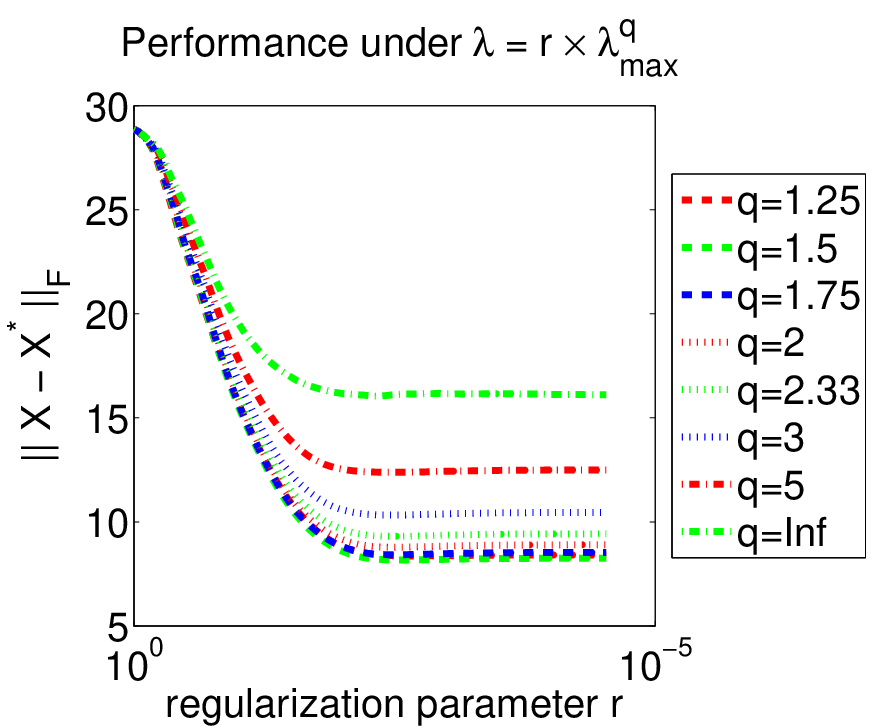
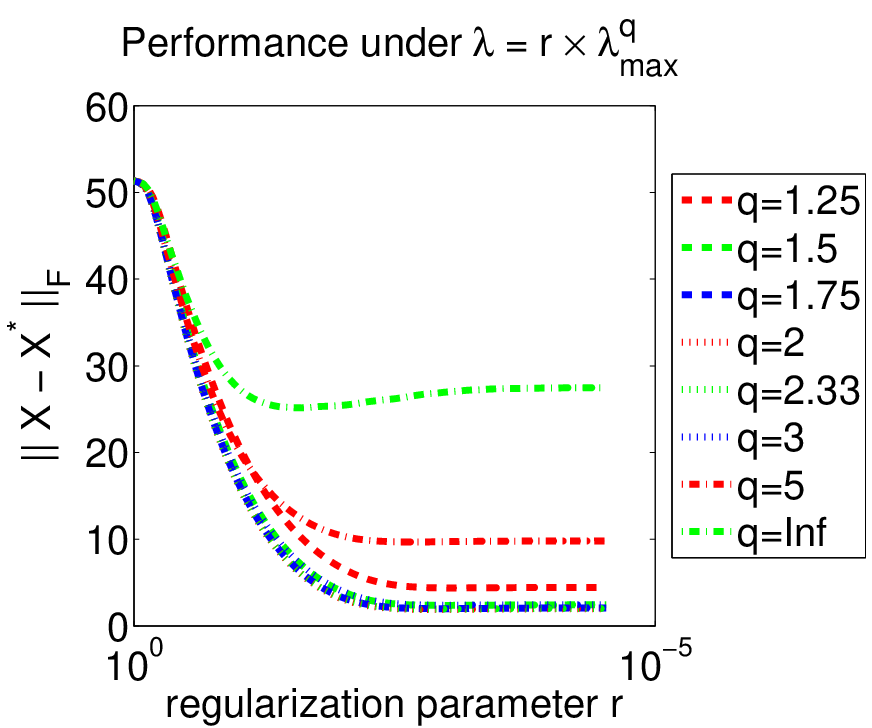


We compute the solutions corresponding to a sequence of decreasing values of , where , for . In addition, we use the solution corresponding to the as the “warm” start for . We report the results in Figure 2, from which we can observe: 1) the distance between the solution and the truth usually decreases with decreasing values of ; 2) for the uniform distribution (see the plots in the first row), performs the best; 3) for the normal distribution (see the plots in the second row), and 3 achieve comparable performance and perform better than , 5 and ; 4) with a properly chosen threshold, the support of can be exactly recovered by the -norm regularization with an appropriate value of , e.g., for the uniform distribution, and for the normal distribution; and 5) the recovery of with nonzero entries drawn from the normal distribution is easier than that with entries generated from the uniform distribution.
The existing theoretical results [17, 23] can not tell which is the best; and we believe that the optimal depends on the distribution of , as indicated from the above results. Therefore, it is necessary to conduct the distribution-specific theoretical studies (note that the previous studies usually make no assumption on ). The proposed GLEP1q algorithm shall help verify the theoretical results to be established.
3.2 Performance on the Letter Data Set
We apply the proposed GLEP1q algorithm for multi-task learning on the Letter data set [29], which consists of 45,679 samples from 8 default tasks of two-class classification problems for the handwritten letters: c/e, g/y, m/n, a/g, i/j, a/o, f/t, h/n. The writings were collected from over 180 different writers, with the letters being represented by binary pixel images. We use the least squares loss for .


3.2.1 Efficiency Comparison with Spg
We compare GLEP1q with the Spg algorithm proposed in [4]. Spg is a specialized solver for the -ball constrained optimization problem, and has been shown to outperform existing algorithms based on blockwise coordinate descent and projected gradient. In Figure 3, we report the computational time under different values of (the number of samples) and (). It is clear from the plots that GLEP1q is much more efficient than Spg, which may attribute to: 1) GLEP1q has a better convergence rate than Spg; and 2) when , the EP1q in GLEP1q can be computed analytically (see Remark 1), while this is not the case in Spg.
3.2.2 Efficiency under Different Values of
We report the computational time (seconds) of GLEP1q under different values of , and (the number of samples) in Figure 4. We can observe from this figure that the computational time of GLEP1q under different values of (for fixed and ) is comparable. Together with the result on the comparison with Spg for , this experiment shows the promise of GLEP1q for solving large-scale problems for any .


3.2.3 Performance under Different Values of
We randomly divide the Letter data into three non-overlapping sets: training, validation, and testing. We train the model using the training set, and tune the regularization parameter on the validation set, where is chosen from . On the testing set, we compute the balanced error rate [11]. We report the results averaged over 10 runs in Figure 5. The title of each plot indicates the percentages of samples used for training, validation, and testing. The results show that, on this data set, a smaller value of achieves better performance.
4 Conclusion
In this paper, we propose the GLEP1q algorithm for solving the -norm regularized problem, for any . The main technical contribution of this paper is the efficient algorithm for the -norm regularized Euclidean projection (EP1q), which is a key building block of GLEP1q. Specifically, we analyze the key theoretical properties of the solution of EP1q, based on which we develop an efficient algorithm for EP1q by solving two zero finding problems. Our analysis also reveals why EP1q for the general is significantly more challenging than the special cases such as .
In this paper, we focus on the efficient implementation of the -regularized problem. We plan to study the effectiveness of the regularization under different values of for real-world applications in computer vision and bioinformatics. We also plan to conduct the distribution-specific [8] theoretical studies for different values of .
References
- [1] A. Argyriou, T. Evgeniou, and Massimiliano Pontil. Convex multi-task feature learning. Machine Learning, 73(3):243–272, 2008.
- [2] F. Bach. Consistency of the group lasso and multiple kernel learning. Journal of Machine Learning Research, 9:1179–1225, 2008.
- [3] A. Beck and M. Teboulle. A fast iterative shrinkage-thresholding algorithm for linear inverse problems. SIAM Journal on Imaging Sciences, 2(1):183–202, 2009.
- [4] E. Berg, M. Schmidt, M. P. Friedlander, and K. Murphy. Group sparsity via linear-time projection. Tech. Rep. TR-2008-09, Department of Computer Science, University of British Columbia, Vancouver, July 2008.
- [5] S. Boyd, L. Xiao, and A. Mutapcic. Subgradient methods: Notes for ee392o, 2003.
- [6] J. Duchi and Y. Singer. Boosting with structural sparsity. In International Conference on Machine Learning, 2009.
- [7] J. Duchi and Y. Singer. Online and batch learning using forward backward splitting. Journal of Machine Learning Research, 10:2899–2934, 2009.
- [8] Y. Eldar and H. Rauhut. Average case analysis of multichannel sparse recovery using convex relaxation. IEEE Transactions on Information Theory, 56(1):505–519, 2010.
- [9] J. Friedman, T. Hastie, and R. Tibshirani. Regularized paths for generalized linear models via coordinate descent. Technical report, Department of Statistics, Stanford University, 2008.
- [10] J. Friedman, T. Hastie, and R. Tibshirani. A note on the group lasso and a sparse group lasso. Technical report, Department of Statistics, Stanford University, 2010.
- [11] I. Guyon, A. B. Hur, S. Gunn, and G. Dror. Result analysis of the nips 2003 feature selection challenge. In Neural Information Processing Systems, pages 545–552, 2004.
- [12] E.T. Hale, W. Yin, and Y. Zhang. Fixed-point continuation for -minimization: Methodology and convergence. SIAM Journal on Optimization, 19(3):1107–1130, 2008.
- [13] J. Hiriart-Urruty and C. Lemaréchal. Convex Analysis and Minimization Algorithms I & II. Springer Verlag, Berlin, 1993.
- [14] M. Kowalski. Sparse regression using mixed norms. Applied and Computational Harmonic Analysis, 27(3):303–324, 2009.
- [15] J. Langford, L. Li, and T. Zhang. Sparse online learning via truncated gradient. Journal of Machine Learning Research, 10:777–801, 2009.
- [16] H. Liu, M. Palatucci, and J. Zhang. Blockwise coordinate descent procedures for the multi-task lasso, with applications to neural semantic basis discovery. In International Conference on Machine Learning, 2009.
- [17] H. Liu and J. Zhang. On the - regularized regression. Technical report, Department of Statistics, Carnegie Mellon University, 2009.
- [18] J. Liu, S. Ji, and J. Ye. Multi-task feature learning via efficient -norm minimization. In Uncertainty in Artificial Intelligence, 2009.
- [19] J. Liu, S. Ji, and J. Ye. SLEP: Sparse Learning with Efficient Projections. Arizona State University, 2009.
- [20] J. Liu and J. Ye. Efficient Euclidean projections in linear time. In International Conference on Machine Learning, 2009.
- [21] L. Meier, S. Geer, and P. Bühlmann. The group lasso for logistic regression. Journal of the Royal Statistical Society: Series B, 70:53–71, 2008.
- [22] J.-J. Moreau. Proximité et dualité dans un espace hilbertien. Bull. Soc. Math. France, 93:273–299, 1965.
- [23] S. Negahban, P. Ravikumar, M. Wainwright, and B. Yu. A unified framework for high-dimensional analysis of -estimators with decomposable regularizers. In Advances in Neural Information Processing Systems, pages 1348–1356. 2009.
- [24] S. Negahban and M. Wainwright. Joint support recovery under high-dimensional scaling: Benefits and perils of -regularization. In Advances in Neural Information Processing Systems, pages 1161–1168. 2008.
- [25] A. Nemirovski. Efficient methods in convex programming. Lecture Notes, 1994.
- [26] Y. Nesterov. Introductory Lectures on Convex Optimization: A Basic Course. Kluwer Academic Publishers, 2004.
- [27] Y. Nesterov. Gradient methods for minimizing composite objective function. CORE Discussion Paper, 2007.
- [28] Y. Nesterov. Primal-dual subgradient methods for convex problems. Mathematical Programming, 120(1):221–259, 2009.
- [29] G. Obozinski, B. Taskar, and M. I. Jordan. Joint covariate selection for grouped classification. Technical report, Statistics Department, UC Berkeley, 2007.
- [30] A. Quattoni, X. Carreras, M. Collins, and T. Darrell. An efficient projection for ,infinity regularization. In International Conference on Machine Learning, 2009.
- [31] J. Shi, W. Yin, S. Osher, and P. Sajda. A fast algorithm for large scale -regularized logistic regression. Technical report, CAAM TR08-07, 2008.
- [32] R. Tibshirani. Regression shrinkage and selection via the lasso. Journal of the Royal Statistical Society Series B, 58(1):267–288, 1996.
- [33] P. Tseng. Convergence of block coordinate descent method for nondifferentiable minimization. Journal of Optimization Theory and Applications, 109:474–494, 2001.
- [34] P. Tseng and S. Yun. A coordinate gradient descent method for nonsmooth separable minimization. Mathematical Programming, 117(1):387–423, 2009.
- [35] L. Xiao. Dual averaging methods for regularized stochastic learning and online optimization. In Advances in Neural Information Processing Systems, 2009.
- [36] K. Yosida. Functional Analysis. Springer Verlag, Berlin, 1964.
- [37] M. Yuan and Y. Lin. Model selection and estimation in regression with grouped variables. Journal Of The Royal Statistical Society Series B, 68(1):49–67, 2006.
- [38] P. Zhao, G. Rocha, and B. Yu. The composite absolute penalties family for grouped and hierarchical variable selection. Annals of Statistics, 37(6A):3468–3497, 2009.
- [39] P. Zhao and B. Yu. Boosted lasso. Technical report, Statistics Department, UC Berkeley, 2004.