跳到论文正文
W Papers独立论文阅读器 arXiv:1009.4679 论文正文 计算阅读时间 · 0%
引用这篇论文根据当前论文元数据生成,正式投稿前建议核对。


License: arXiv.org perpetual non-exclusive license
arXiv:1009.4679v2 [math.PR] 20 May 2011

Asymptotic of geometrical navigation
on a random set of points of the plane

Nicolas Bonichon Jean-François Marckert\begin{array}[]{ll}\textrm{\Large Nicolas Bonichon}&\textrm{\Large~~~~~~~~~~Jean-Fran\c{c}ois Marckert}\end{array}

CNRS, LaBRI, Université de Bordeaux

351 cours de la Libération

33405 Talence cedex, France

email: name@labri.fr

The first author is partially supported by the ANR project ALADDIN and the second author is partially supported by ANR-08-BLAN-0190-04 A3.

Abstract

A navigation on a set of points SS is a rule for choosing which point to move to from the present point in order to progress toward a specified target. We study some navigations in the plane where SS is a non uniform Poisson point process (in a finite domain) with intensity going to +∞+\infty. We show the convergence of the traveller path lengths, the number of stages done, and the geometry of the traveller trajectories, uniformly for all starting points and targets, for several navigations of geometric nature. Other costs are also considered. This leads to asymptotic results on the stretch factors of random Yao-graphs and random θ\theta-graphs.

1 Introduction

1.1 Navigations

Often, a traveller who can be a human being, a migratory animal, a letter, a radio message, a message in a wireless ad hoc network, … wanting to reach a point tt starting from a point ss has to stop along the route where, according to the case, he can sleep, eat, be sorted, be amplified, or routed. Generally the traveller can not stop everywhere: only some special places offer what is needed (a hostel, a river, a post-office, a radio relay station, a router, …). Often the traveller can not compute the optimal route from its initial position: it has to choose the next point to move to using only some local information. This paper deals with this problem: a random set SS of possible stops given, what happens if a traveller stops “at the first point in SS” which is in the direction of tt up to an angle θ\theta? How many steps are done? What is the total distance done? In this paper we answer these questions in the asymptotic case, when the number of points in SS goes to +∞+\infty.

Formally, consider a traveller on ℝ2\mathbb{R}^{2} beginning its travel at the starting position ss and wanting to reach the target tt using as set of possible stopping places SS, a finite subset of ℝ2\mathbb{R}^{2}. We call navigation11 1 also called in the literature memoryless routing algorithm with set of stopping places SS, a function 𝐗\Nav from ℝ2×ℝ2\mathbb{R}^{2}\times\mathbb{R}^{2} onto ℝ2\mathbb{R}^{2} such that for any (s,t)(s,t), 𝐗⁡(s,t)\Nav(s,t) belongs to S∪{t}S\cup\{t\}, and satisfies moreover 𝐗⁡(s,s)=s\Nav(s,s)=s for any s∈ℝ2s\in\mathbb{R}^{2}. The position 𝐗⁡(s,t){\bf X}(s,t) corresponds to the first stop of the traveller in its travel from ss to tt. Hence,

𝐗⁡(s,t,j):=𝐗⁡(𝐗⁡(s,t,j−1),t),j≥1\Nav(s,t,j):=\Nav(\Nav(s,t,j-1),t),\hskip 20.00003ptj\geq 1

are the successive stops of the traveller, where by convention 𝐗⁡(s,t,j)=s\Nav(s,t,j)=s for j=0j=0. When no confusion is possible on ss, tt and 𝐗\Nav, we will write sjs_{j} instead of 𝐗⁡(s,t,j)\Nav(s,t,j). The quantity

Δ𝐗​(s,t,j):=𝐗⁡(s,t,j)−𝐗⁡(s,t,j−1)\Delta^{\Nav}(s,t,j):=\Nav(s,t,j)-\Nav(s,t,j-1)

is called the jjth stage. For a general navigation algorithm 𝐗\Nav, if #​S<+∞\#S<+\infty, either 𝐗⁡(s,t,j)=t\Nav(s,t,j)=t for jj large enough, or 𝐗⁡(s,t,j)≠t\Nav(s,t,j)\neq t for all jj. In the first case, the global navigation from ss to tt succeeds, whereas in the second case, it fails. In case of success, the (global) path from ss to tt is

𝖯𝖺𝗍𝗁𝐗​(s,t):=(s0,…,s𝖭𝖻𝐗​(s,t)){\sf Path}^{\Nav}(s,t):=\left(s_{0},\dots,s_{{\sf Nb}^{\Nav}(s,t)}\right) (1)

where 𝖭𝖻𝐗​(s,t):=min⁡{j,sj=t}{\sf Nb}^{\Nav}(s,t):=\min\left\{j,~s_{j}=t\right\} is the number of stages needed to go from ss to tt.

We are interested in navigations in ℝ2\mathbb{R}^{2} where the point to move to is chosen according to some rules of geometrical nature: we consider two classes of so-called compass navigations; these navigations select the next stopping place to move to as the “nearest” point of ss in the set S∪{t}S\cup\{t\}, in the “direction” of tt (see Section 1.2).

All along the paper, 𝒟{\cal D} refers to a bounded and simply connected open domain in ℝ2\mathbb{R}^{2}. The sets of considered stopping places SS are finite random subsets of 𝒟{\cal D} taken according to two models: SS will be either the set {p1,…,pn}\{p_{1},\dots,p_{n}\} where the points pip_{i}’s are picked independently according to a distribution having a regular density ff (with respect to the Lebesgue measure) in 𝒟{\cal D} (see Section 2.3.2), or SS will be a Poisson point process with intensity n​fnf, for some n>0n>0 (see Section 1.3).

The main goal of this paper is to study the global asymptotic behaviour of the paths of the traveller. Global means all the possible trajectories corresponding to all starting points ss and targets tt of 𝒟{\cal D} are considered all together. Several quantities are then studied, describing the “deviation” of the paths of the traveller (or functionals of the path, as the length) to a deterministic limit (see Section 1.4). The asymptotic is made on the number of points of SS, which will go to +∞+\infty (that is n→+∞n\to+\infty in one of the models).

Convention

Throughout the paper, the two dimensional real plane ℝ2\mathbb{R}^{2} is identified with the set of complex numbers ℂ\mathbb{C} and according to what appears simpler, the complex notation or the real one is used without warning. The real part, the imaginary part, the modulus of zz are respectively written ℜ⁡(z)\Re(z), ℑ⁡(z)\Im(z), and |z||z|; the argument arg⁡(z)\arg(z) of any real number z≠0z\neq 0 is the unique real number θ\theta in [0,2​π)[0,2\pi) such that z=ρ​ei​θz=\rho e^{i\theta}, for some ρ>0\rho>0 (we set arg⁡(0)=0\arg(0)=0). The characteristic function of the set AA is denoted by 𝟏A{\bf 1}_{A}. Notation ⟦x,y⟧\llbracket x,y\rrbracket refers to the set of integers included in [x,y][x,y] and B⁡(x,r)={y∈ℂ,|x−y|<r}B(x,r)=\{y\in\mathbb{C},~|x-y|<r\} to the open ball with centre xx and radius rr in ℂ\mathbb{C}, the closed ball is B¯​(x,r)\overline{B}(x,r). For x∈ℂx\in\mathbb{C}, A⊂ℂA\subset\mathbb{C}, d⁡(x,A)=inf{|x−y|,y∈A}d(x,A)=\inf\{|x-y|,y\in A\}.

1.2 Two types of navigations

The two types of navigation introduced below, namely cross navigation and straight navigation, may appear very similar, but their asymptotic behaviours as well as their analysis are quite different.

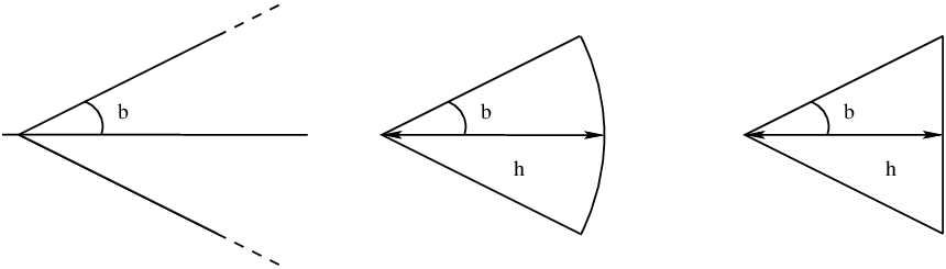
For any β∈(0,2​π)\beta\in(0,2\pi), as illustrated on Fig. 1, let

𝖲𝖾𝖼𝗍⁡(β)\displaystyle{\sf Sect}(\beta) :⁣=\displaystyle:= {ρ​ei​ν,ρ>0,|ν|≤β/2},\displaystyle\left\{\rho e^{i\nu},~\rho>0,|\nu|\leq\beta/2\right\},
𝖢𝖺𝗆​(β)​(h)\displaystyle{\sf Cam}(\beta)(h) :⁣=\displaystyle:= 𝖲𝖾𝖼𝗍​(β)∩B¯​(0,h),\displaystyle{\sf Sect}(\beta)\cap\overline{B}(0,h), (2)
𝖳𝗋𝗂​(β)​(h)\displaystyle{\sf Tri}(\beta)(h) :⁣=\displaystyle:= {x+i​y,x∈(0,h],y∈ℝ,|y|≤x​tan⁡(β/2)}.\displaystyle\left\{x+iy,~x\in(0,h],y\in\mathbb{R},|y|\leq x\tan(\beta/2)\right\}.

Notation 𝖢𝖺𝗆{\sf Cam} and 𝖳𝗋𝗂{\sf Tri} are short version for “Camembert portion” and “triangle”.
Refer to caption


Figure 1: Representation of 𝖲𝖾𝖼𝗍​(β),𝖳𝗋𝗂​(β)​(h){\sf Sect}(\beta),{\sf Tri}(\beta)(h) and 𝖢𝖺𝗆​(β)​(h){\sf Cam}(\beta)(h). Notice that each peak point of the figures is excluded from the corresponding set.

1.2.1 First type of navigations: Cross navigations

Cross navigations are parametrised by a parameter θ\theta satisfying θ=2​π/pθ\theta=2\pi/p_{\theta} for some pθ∈{3,4,…}p_{\theta}\in\{3,4,\dots\}. For any x∈ℂx\in\mathbb{C}, for κ\kappa in⟦0,pθ−1⟧\llbracket 0,p_{\theta}-1\rrbracket the κ\kappath angular sector around xx is

𝖲𝖾𝖼𝗍⁡[κ,x]:=x+ei​κ​θ​𝖲𝖾𝖼𝗍​(θ).{\sf Sect}[\kappa,x]:=x+e^{i\kappa\theta}{\sf Sect}(\theta).

The two half-lines HLκ⁡(x)\HL_{\kappa}(x) and HLκ+1⁡(x)\HL_{\kappa+1}(x) defined by

HLj(x):=x+{ρei​θ​(j−1/2),ρ>0},j∈⟦0,pθ⟧,\HL_{j}(x):=x+\left\{\rho e^{i\theta(j-1/2)},~\rho>0\right\},~~~j\in\llbracket 0,p_{\theta}\rrbracket, (3)

are called the first and last border of 𝖲𝖾𝖼𝗍⁡[κ,x]{\sf Sect}[\kappa,x]. As illustrated in Fig. 2, for h>0h>0, the κ\kappath triangle and κ\kappath Camembert section around zz with height hh are respectively:

𝖳𝗋𝗂​[κ,x]​(h)\displaystyle{{\sf Tri}}[\kappa,x](h) :⁣=\displaystyle:= x+ei​κ​θ​𝖳𝗋𝗂​(θ)​(h),𝖢𝖺𝗆⁡[κ,x]​(h):=x+ei​κ​θ​𝖢𝖺𝗆​(θ)​(h),\displaystyle x+e^{i\kappa\theta}{\sf Tri}(\theta)(h),~~~~{{\sf Cam}}[\kappa,x](h):=x+e^{i\kappa\theta}{\sf Cam}(\theta)(h),

where for any z1,z2∈ℂz_{1},z_{2}\in\mathbb{C}, and any A⊂ℂA\subset\mathbb{C}, z1+z2​Az_{1}+z_{2}A is the set {z1+z2​y,y∈A}\{z_{1}+z_{2}y,~y\in A\}.

Refer to caption


Figure 2: Representation of the 6 angular sectors around a point xx with pθ=6p_{\theta}=6; on the second picture, representation of 𝖳𝗋𝗂​[0,x]​(h){{\sf Tri}}[0,x](h), and on the third 𝖢𝖺𝗆​[0,x]​(h){{\sf Cam}}[0,x](h).

As one can see on Fig. 2, the half-lines (HLκ(t),κ∈⟦1,pθ⟧)(\HL_{\kappa}(t),\kappa\in\llbracket 1,p_{\theta}\rrbracket), forms a cross around tt that we denote by 𝖢𝗋𝗈𝗌𝗌⁡(t):=⋃κ=1pθHLκ⁡(t).{\sf Cross}(t):=\bigcup_{\kappa=1}^{p_{\theta}}\HL_{\kappa}(t). This justifies the terminology “cross navigation”.

Let ss and tt in 𝒟{\cal D}, and let κ\kappa be such that t∈𝖲𝖾𝖼𝗍⁡[κ,s]t\in{\sf Sect}[\kappa,s]. Consider 𝐁κ​(s)={s+r​ei​κ​θ,r≥0}{\bf B}_{\kappa}(s)=\{s+re^{i\kappa\theta},~r\geq 0\} the bisecting half-line of 𝖲𝖾𝖼𝗍⁡[κ,s]{\sf Sect}[\kappa,s]. Consider the lines parallel to HLκ⁡(s)\HL_{\kappa}(s) and HLκ+1⁡(s)\HL_{\kappa+1}(s) passing via tt. These two lines intersect the half-line 𝐁κ​(s){\bf B}_{\kappa}(s) in two points.

Refer to caption


Figure 3: Representation I⁡(s,t)I(s,t), 𝐁κ​(s){\bf B}_{\kappa}(s). Γ⁡(s,t)\Gamma(s,t) is represented by the heavy segments.

The point which is the closest from ss is called I⁡(s,t)I(s,t), as represented on Fig. 3. The compact Γ⁡(s,t)\Gamma(s,t) is:

Γ⁡(s,t):=[s,I⁡(s,t)]∪[I⁡(s,t),t].\Gamma(s,t):=[s,I(s,t)]\cup[I(s,t),t]. (4)

pθp_{\theta} Yao navigation and pθp_{\theta} CT navigation, noted 𝐂𝐘{\bf CY} and 𝐂𝐓{\bf CT} are defined given a set of stopping places SS, a finite subset of ℝ2\mathbb{R}^{2}.

Definition of pθp_{\theta} Yao navigation

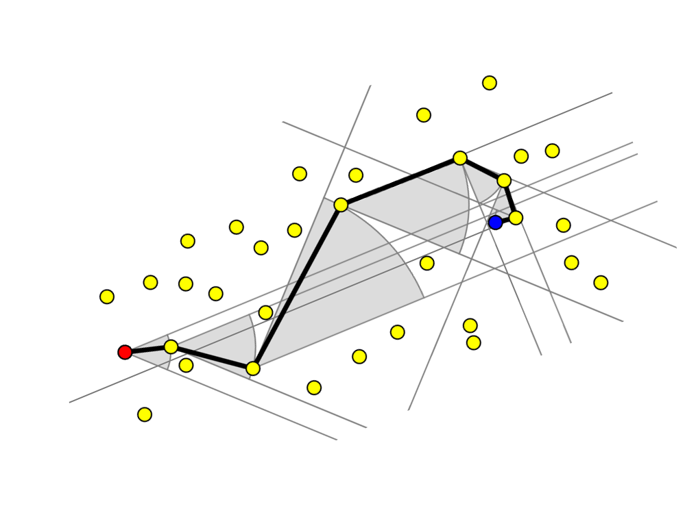
For (s,t)∈ℝ2×ℝ2(s,t)\in\mathbb{\mathbb{R}}^{2}\times\mathbb{\mathbb{R}}^{2}, consider the smallest integer κ\kappa in ⟦0,pθ−1⟧\llbracket 0,p_{\theta}-1\rrbracket such that tt lies in 𝖲𝖾𝖼𝗍⁡[κ,s]{\sf Sect}[\kappa,s]. Consider the smallest rr such that 𝖢𝖺𝗆⁡[κ,s]​(r)∩(S∪{t}){{\sf Cam}}[\kappa,s](r)\cap\left(S\cup\{t\}\right) is not empty. We set 𝐂𝐘⁡(s,t)=z{\bf CY}(s,t)=z, the element of 𝖢𝖺𝗆⁡[κ,s]​(r)∩(S∪{t}){{\sf Cam}}[\kappa,s](r)\cap\left(S\cup\{t\}\right) that is the closest of the first border of 𝖲𝖾𝖼𝗍⁡[κ,s]{\sf Sect}[\kappa,s] (see Fig. 4 (a)).

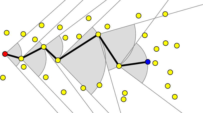
Refer to caption Refer to caption


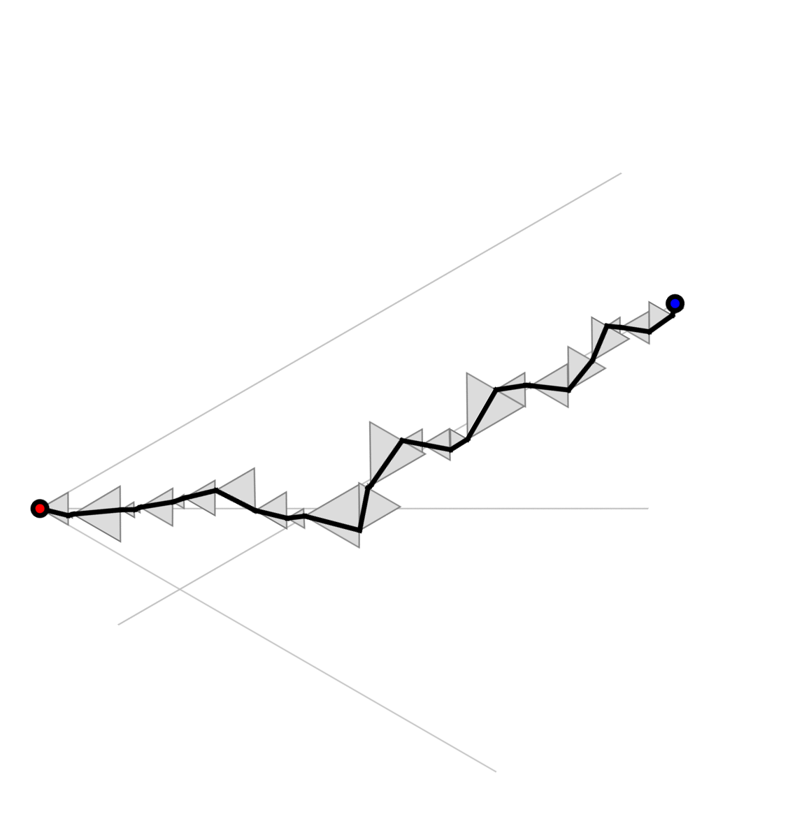
Figure 4: (a) An example of Yao navigation with pθ=8p_{\theta}=8 the starting point is on the left. Are drawn the decision domains for each stage, and the sectors that contain the destination. (b) An example of Yao straight navigation with θ=π/2\theta=\pi/2 the starting point is on the left. Are drawn the decision domains for each stage, and the sectors that contain the destination.

This navigation appears to be the canonical navigation in Yao’s graphs [19].

Definition of pθp_{\theta} CT navigation

pθp_{\theta} CT navigation is a simple variant of pθp_{\theta} Yao navigation. It is defined as pθp_{\theta} Yao navigation, except that 𝖳𝗋𝗂​[κ,s]​(r){{\sf Tri}}[\kappa,s](r) replaces 𝖢𝖺𝗆​[κ,s]​(r){{\sf Cam}}[\kappa,s](r).

Comments 1

If tt belongs to HLκ⁡(s)\HL_{\kappa}(s) then tt lies in both 𝖲𝖾𝖼𝗍⁡[κ,s]{\sf Sect}[\kappa,s] and 𝖲𝖾𝖼𝗍⁡[κ−1modpθ,s]{\sf Sect}[\kappa-1\mod p_{\theta},s]; in the other cases, tt belongs to a unique sector 𝖲𝖾𝖼𝗍⁡[κ,s]{\sf Sect}[\kappa,s]. In the sequel, the domains 𝖢𝖺𝗆​[κ,s]​(r){{\sf Cam}}[\kappa,s](r) and 𝖳𝗋𝗂​[κ,s]​(r){{\sf Tri}}[\kappa,s](r) which are, depending on the algorithm considered, the minimum domains allowing to decide to which point to move to, are called the decision domains.

1.2.2 Second type of navigations: Straight navigation

Straight navigations are closer to real traveller strategies: the stopping places are chosen not too far from the segment leading to the target. We set two straight navigations, parametrised by a real number θ∈(0,2​π)\theta\in(0,2\pi). The difference between the following objects and those before defined is that the sectors are oriented such that their bisecting lines are the straight line (s,t)(s,t):

𝖲𝖾𝖼𝗍→​(s,t)\displaystyle\overrightarrow{{\sf Sect}}(s,t) :⁣=\displaystyle:= s+exp⁡(i​arg⁡(t−s))​𝖲𝖾𝖼𝗍​(θ),\displaystyle s+\exp(i\arg(t-s))\,{\sf Sect}(\theta),
𝖢𝖺𝗆→​(s,t)​(h)\displaystyle\overrightarrow{{\sf Cam}}(s,t)(h) :⁣=\displaystyle:= s+exp⁡(i​arg⁡(t−s))​𝖢𝖺𝗆​(θ)​(h),\displaystyle s+\exp(i\arg(t-s))\,{\sf Cam}(\theta)(h),
𝖳𝗋𝗂→​(s,t)​(h)\displaystyle\overrightarrow{{\sf Tri}}(s,t)(h) :⁣=\displaystyle:= s+exp⁡(i​arg⁡(t−s))​𝖳𝗋𝗂​(θ)​(h).\displaystyle s+\exp(i\arg(t-s))\,{\sf Tri}(\theta)(h).

θ\theta Straight Yao navigation and θ\theta Straight T navigation will be denoted 𝐒𝐘{\bf SY} and 𝐒𝐓{\bf ST}.

θ\theta Straight Yao navigation

For (s,t)∈S2(s,t)\in S^{2}, consider the smallest rr such that the set 𝖢𝖺𝗆→​(s,t)​(r)∩(S∪{t})\overrightarrow{{\sf Cam}}(s,t)(r)\cap(S\cup\{t\}) is not empty. Set 𝐒𝐘⁡(s,t)=z{\bf SY}(s,t)=z, where zz is the closest of the first border of 𝖢𝖺𝗆→​(s,t)\overrightarrow{{\sf Cam}}(s,t) (see Fig. 4 (b)).

θ\theta Straight T navigation

The θ\theta Straight T navigation 𝐒𝐓{\bf ST} is similarly defined except that 𝖳𝗋𝗂→​(s,t)​(r)\overrightarrow{{\sf Tri}}(s,t)(r) replaces 𝖢𝖺𝗆→​(s,t)​(r)\overrightarrow{{\sf Cam}}(s,t)(r).

1.3 The model of random stopping places set: a Poisson point process

Denote by Lip⋆⁡(𝒟)\Lip^{\star}({\cal D}) the set of Lipschitz functions f:𝒟→ℝ+f:{\cal D}\to\mathbb{R}^{+} with a positive infimum on 𝒟{\cal D}: a function ff is in Lip⋆⁡(𝒟)\Lip^{\star}({\cal D}), if there exists αf>0\alpha_{f}>0, such that |f⁡(x)−f⁡(y)|≤αf​|x−y||f(x)-f(y)|\leq\alpha_{f}|x-y| for all x,y∈𝒟x,y\in{\cal D}, and mf:=inf{f⁡(x),x∈𝒟}>0m_{f}:=\inf\{f(x),x\in{\cal D}\}>0. Since 𝒟{\cal D} is bounded, Mf:=max⁡{f⁡(x),x∈𝒟}<+∞M_{f}:=\max\{f(x),x\in{\cal D}\}<+\infty.

In this paper, we consider a Poisson point processes 𝐒⁡(f){\bf S}(f) whose intensity measure μf\mu_{f} on 𝒟{\cal D} is μf​(A)=∫Af⁡(z)​𝑑z\mu_{f}(A)=\int_{A}f(z)dz, for some f∈Lip⋆⁡(𝒟)f\in\Lip^{\star}({\cal D}) (in words, μf\mu_{f} has density ff with respect to the Lebesgue measure on ℝ2\mathbb{R}^{2}): the necessity of the Lipschitz condition will clearly appear later on, with the appearance of a differential equation. The distribution of 𝐒⁡(f){\bf S}(f) is denoted by ℙf\mathbb{P}_{f}. Since 𝐒⁡(f){\bf S}(f) has no multiple points a.s., #​𝐒​(f)∼𝖯𝗈𝗂𝗌𝗌𝗈𝗇⁡(∫𝒟f⁡(u)​𝑑u)\#{\bf S}(f)\sim{\sf Poisson}(\int_{\cal D}f(u)du). For any disjoint Borelian subsets B1,…,BkB_{1},\dots,B_{k} of ℝ2\mathbb{R}^{2}, (𝐒⁡(f)∩B1),…,(𝐒⁡(f)∩Bk)({\bf S}(f)\cap B_{1}),\dots,({\bf S}(f)\cap B_{k}) are independent and #⁡(𝐒⁡(f)∩Bj)∼𝖯𝗈𝗂𝗌𝗌𝗈𝗇⁡(∫Bjf⁡(u)​𝑑u)\#\left({\bf S}(f)\cap B_{j}\right)\sim{\sf Poisson}\left(\int_{B_{j}}f(u)\ du\right) (for more explanations on PPP, see Chap. 10 in [12]). As usual, a representation of the set 𝐒⁡(f){\bf S}(f) is as follows: 𝐒⁡(f)={x1,…,x𝐧}{\bf S}(f)=\{x_{1},\dots,x_{\bf n}\}, where 𝐧∼𝖯𝗈𝗂𝗌𝗌𝗈𝗇⁡(∫𝒟f){\bf n}\sim{\sf Poisson}(\int_{{\cal D}}f), and where the x1,x2,…,x_{1},x_{2},\dots, are i.i.d. and independent of 𝐧{\bf n}, and each xix_{i} has density f/inf𝒟ff/\inf_{{\cal D}}f.

In the paper, we assume the measure ∑x∈𝐒⁡(f)δx\sum_{x\in{\bf S}(f)}\delta_{x} defined on a probability space (Ω,𝒜,ℙ)(\Omega,{\cal A},\mathbb{P}), and is considered as a random variable taking its values in 𝖭{\sf N} the set of counting measures in ℂ\mathbb{C}, equipped with the σ\sigma-field 𝒩\mathcal{N} generated by the sets EB,k={μ,μ⁡(B)=k}E_{B,k}=\{\mu,\mu(B)=k\} for compacts sets B⊂ℂB\subset\mathbb{C}, kk integer.

The model consisting of nn i.i.d. points chosen according to a density ff is considered in Section 2.3.2.

Comments 2

The navigations 𝐗\Nav we study, as well as the function 𝖯𝖺𝗍𝗁𝐗{\sf Path}^{\Nav}, 𝖯𝗈𝗌𝐗{\sf Pos}^{\Nav}, and various cost functions are all defined given a stopping places set SS, and then, there are some functions of SS (one should write 𝐗⁡(S)\Nav(S), etc. but we choose to delete this SS to lighten the notation). On (Ω,𝒜,ℙ)(\Omega,{\cal A},\mathbb{P}), these functions are random variables with values in some functional spaces.

1.4 Quantities of interest

In (1) is defined 𝖯𝖺𝗍𝗁𝐗​(s,t){\sf Path}^{\bf X}(s,t). In many applications, a quantity of interest is the comparison between the Euclidean distance |s−t||s-t| and the path length, the total distance done by the traveller in case of success:

|𝖯𝖺𝗍𝗁𝐗​(s,t)|:=∑j=1𝖭𝖻𝐗​(s,t)|sj−sj−1|.|{\sf Path}^{\bf X}(s,t)|:=\sum_{j=1}^{{\sf Nb}^{\bf X}(s,t)}|s_{j}-s_{j-1}|.

The associated trajectory is the compact subset of ℝ2\mathbb{R}^{2} formed by the union of the segments [sj,sj+1][s_{j},s_{j+1}]:

[𝖯𝖺𝗍𝗁𝐗​(s,t)]:=⋃j=1𝖭𝖻𝐗​(s,t)[sj−1,sj].[{\sf Path}^{\bf X}(s,t)]:=\bigcup_{j=1}^{{\sf Nb}^{\bf X}(s,t)}[s_{j-1},s_{j}].

One of the results of the paper is the comparison between [𝖯𝖺𝗍𝗁𝐗​(s,t)][{\sf Path}^{\bf X}(s,t)] and a limiting object.

If the point process is not homogeneous, the evaluation of the traveller’s trajectory calls for a precise study of the traveller’s speed. We introduce the function 𝖯𝗈𝗌s,t𝐗:[0,𝖭𝖻𝐗​(s,t)]→ℝ2{\sf Pos}_{s,t}^{\Nav}:[0,{\sf Nb}^{\bf X}(s,t)]\to\mathbb{R}^{2} whose values coincides with those of 𝐗(s,t,.)\Nav(s,t,.) at integer points, and interpolated in between. Hence, 𝖯𝗈𝗌s,t𝐗{\sf Pos}_{s,t}^{\bf X} gives the position of the traveller according to the number of stages; for any s,t∈𝒟s,t\in{\cal D}, [𝖯𝖺𝗍𝗁𝐗​(s,t)][{\sf Path}^{\bf X}(s,t)] equals the range of 𝖯𝗈𝗌s,t𝐗{\sf Pos}_{s,t}^{\bf X}. From our point of view, the asymptotic results obtained for 𝖯𝗈𝗌s,t{\sf Pos}_{s,t} are among the main contributions of this paper.

In some applications, the sum of a function of the stage lengths appears to be the relevant quantity instead of the length. Formally a “unitary cost function” H:ℂ→ℝH:\mathbb{C}\to\mathbb{R} is considered. The total cost associated with HH corresponding to 𝖯𝖺𝗍𝗁𝐗​(s,j)=(s0,…,s𝖭𝖻𝐗​(s,t)){\sf Path}^{\bf X}(s,j)=\left(s_{0},\dots,s_{{\sf Nb}^{\bf X}(s,t)}\right) is

𝖢𝗈𝗌𝗍H𝐗​(s,t):=∑j=1𝖭𝖻𝐗​(s,t)H⁡(sj−sj−1).{\sf Cost}_{H}^{\bf X}(s,t):=\sum_{j=1}^{{\sf Nb}^{\bf X}(s,t)}H\left(s_{j}-s_{j-1}\right). (5)

Important elementary cost functions are H:x→|x|H:x\to|x| which gives 𝖢𝗈𝗌𝗍H​(s,t)=|𝖯𝖺𝗍𝗁⁡(s,t)|{\sf Cost}_{H}(s,t)=|{\sf Path}(s,t)|, the function H:x→1H:x\to 1 which gives 𝖢𝗈𝗌𝗍H𝐗​(s,t)=𝖭𝖻𝐗​(s,t){\sf Cost}_{H}^{\bf X}(s,t)={\sf Nb}^{\bf X}(s,t), and functions of the type H⁡(x)=|x|βH(x)=|x|^{\beta} which corresponds, at least for some β\beta, to some real applications.

2 Statements of the main results

In the rest of the paper, ff is a fixed element of Lip⋆⁡(𝒟)\Lip^{\star}({\cal D}) and aa a fixed positive number. The set 𝒟⁡[a]:={x∈𝒟:d⁡(x,∁​𝒟)≥a}{\cal D}[a]:=\left\{x\in{\cal D}~:d(x,\complement{\cal D})\geq a\right\} is the set of points in 𝒟{\cal D} at distance at least aa to ∁​𝒟\complement{\cal D}, the complement of 𝒟{\cal D}. The asymptotic behaviour of 𝖯𝖺𝗍𝗁𝐗​(s,t){\sf Path}^{\Nav}(s,t) (when the set of stopping places SS increases) is difficult to predict if the limiting trajectories between ss and tt are too close of ∁​𝒟\complement{\cal D}. We then set a notation to designate the pairs (s,t)(s,t) that can be treated. Set

𝒟′​[a]:={(s,t)∈𝒟2:Z⁡(s,t)⊂𝒟⁡[a]},{\cal D}^{\prime}[a]:=\{(s,t)\in{\cal D}^{2}~:Z(s,t)\subset{\cal D}[a]\},

where according to the context Z⁡(s,t)=Γ⁡(s,t)Z(s,t)=\Gamma(s,t) (in case cross navigations are concerned) or Z⁡(s,t)=[s,t]Z(s,t)=[s,t] (in case straight ones are concerned). Some other restrictions concerning θ\theta will be added in order to avoid situations where the navigation can fail.

Before giving the results, we define some constants, computed in Sections 3.3.1 and 3.3.3, and related to the speed of the traveller along its trajectory, and to some ratio “mean length of a stage” divided by “length of the projection of a stage” with respect to some ad hoc directions.

𝐂𝐛𝐢𝐬𝐒𝐓=𝐂𝐛𝐢𝐬𝐂𝐓=12​πtan⁡(θ/2)𝐂𝐛𝐢𝐬𝐒𝐘=𝐂𝐛𝐢𝐬𝐂𝐘=2​π​sin⁡(θ/2)θ3/2𝐂𝐛𝐨𝐫𝐂𝐓=π​cos3⁡(θ/2)4​sin⁡(θ/2)𝐂𝐛𝐨𝐫𝐂𝐘=π/2​sin⁡(θ)θ3/2𝐐𝐛𝐢𝐬𝐒𝐓=𝐐𝐛𝐢𝐬𝐂𝐓=12​(1cos⁡(θ/2)+arcsinh⁡(tan⁡(θ/2))tan⁡(θ/2))𝐐𝐛𝐢𝐬𝐒𝐘=𝐐𝐛𝐢𝐬𝐂𝐘=θ/2sin⁡(θ/2)𝐐𝐛𝐨𝐫𝐂𝐓=12​(1cos2⁡(θ/2)+arcsinh⁡(tan⁡(θ/2))sin⁡(θ/2))𝐐𝐛𝐨𝐫𝐂𝐘=θsin⁡(θ)\begin{array}[]{|l|l|}\hline\cr{\bf C_{bis}^{{\bf ST}}}={\bf C_{bis}^{{\bf CT}}}=\frac{1}{2}\sqrt{\frac{\pi}{\tan(\theta/2)}}&{\bf C_{bis}^{{\bf SY}}}={\bf C_{bis}^{{\bf CY}}}=\frac{\sqrt{2\pi}\sin(\theta/2)}{\theta^{3/2}}\\ \hline\cr{\bf C_{bor}^{{\bf CT}}}=\sqrt{\frac{\pi\cos^{3}(\theta/2)}{4\,\sin(\theta/2)}}&{\bf C_{bor}^{{\bf CY}}}=\frac{\sqrt{\pi/2}\sin(\theta)}{\theta^{3/2}}\\ \hline\cr{\bf Q_{bis}^{{\bf ST}}}={\bf Q_{bis}^{{\bf CT}}}=\frac{1}{2}\left(\frac{1}{\cos(\theta/2)}+\frac{\arcsinh(\tan(\theta/2))}{\tan(\theta/2)}\right)&{\bf Q_{bis}^{{\bf SY}}}={\bf Q_{bis}^{{\bf CY}}}=\frac{\theta/2}{\sin(\theta/2)}\\ \hline\cr{\bf Q_{bor}^{{\bf CT}}}=\frac{1}{2}\left(\frac{1}{\cos^{2}(\theta/2)}+\frac{\arcsinh(\tan(\theta/2))}{\sin(\theta/2)}\right)&{\bf Q_{bor}^{{\bf CY}}}=\frac{\theta}{\sin(\theta)}\\ \hline\cr\end{array} (6)

2.1 Limit theorems for the straight navigations

The first theorem uniformly compares the path length |𝖯𝖺𝗍𝗁𝐗​(s,t)||{\sf Path}^{\bf X}(s,t)| with a multiple of |s−t||s-t|.

Theorem 3

Let 𝐗=𝐒𝐘{\bf X}={\bf SY} and θ<π/2\theta<\pi/2, or 𝐗=𝐒𝐓{\bf X}={\bf ST} and θ≤π/2\theta\leq\pi/2. For any α∈(0,1/8)\alpha\in(0,1/8), any β>0\beta>0, for nn large enough

ℙn​f​(sup(s,t)∈𝒟′​[a]||𝖯𝖺𝗍𝗁𝐗​(s,t)|−𝐐𝐛𝐢𝐬𝐗×|s−t||≥n−α)≤n−β.\mathbb{P}_{nf}\left(\sup_{(s,t)\in{\cal D}^{\prime}[a]}\big||{\sf Path}^{{\bf X}}(s,t)|-{\bf Q_{bis}^{{\bf X}}}\times|s-t|\big|\geq n^{-\alpha}\right)\leq n^{-\beta}.

The terms 𝐐𝐛𝐢𝐬𝐒𝐓{\bf Q_{bis}^{{\bf ST}}} and 𝐐𝐛𝐢𝐬𝐒𝐘{\bf Q_{bis}^{{\bf SY}}} “measures” the efficiency of the traveller with respect to the direction of the bisecting lines of the decision sectors used.

We now describe the asymptotic behavior of 𝖯𝗈𝗌s,t𝐗{\sf Pos}_{s,t}^{\bf X}. In the case of straight navigation, the limiting position function 𝖯𝗈𝗌∞,c{\sf Pos}^{\infty,c} is the deterministic solution of a differential equation, and depends on a real parameter cc function of θ\theta and of 𝐗{\bf X}.

For any (λ,ν)∈(0,+∞)×[0,2​π](\lambda,\nu)\in(0,+\infty)\times[0,2\pi], let Fλ,νF_{\lambda,\nu} be the function from 𝒟{\cal D} into ℂ\mathbb{C} defined by

Fλ,ν​(z):=λ​ei​ν/f⁡(z).F_{\lambda,\nu}(z):={\lambda e^{i\nu}}/{\sqrt{f(z)}}. (7)

For s0∈𝒟s_{0}\in{\cal D} given, consider the following ordinary differential equation

ODE⁡(λ,ν,s0):={ρ⁡(0)=s0,∂ρ⁡(x)∂x=Fλ,ν​(ρ⁡(x)).\ODE(\lambda,\nu,s_{0}):=\left\{\begin{array}[]{l}\rho(0)=s_{0},\\ \displaystyle\frac{\partial\rho(x)}{\partial x}=F_{\lambda,\nu}(\rho(x)).\end{array}\right. (8)

By Cauchy-Lipschitz Theorem, ODE⁡(λ,ν,s0)\ODE(\lambda,\nu,s_{0}) admits a unique solution x↦SOLs0λ,ν⁡(x)x\mapsto\SOL_{s_{0}}^{\lambda,\nu}(x) valid for x≥0x\geq 0 and while SOLs0λ,ν⁡(x)\SOL_{s_{0}}^{\lambda,\nu}(x) stays inside 𝒟{\cal D}; indeed since ff is in Lip⋆⁡(𝒟)\Lip^{\star}({\cal D}), so do Fλ,νF_{\lambda,\nu}. Since ff takes its values in ℝ+\mathbb{R}^{+}, arg⁡(Fλ,ν)=ν\arg(F_{\lambda,\nu})=\nu. Hence, SOLs0λ,ν\SOL_{s_{0}}^{\lambda,\nu} appears to be a monotone parametrisation of the segment {s0+x​ei​ν,x>0}∩𝒟\{s_{0}+xe^{i\nu},~x>0\}\cap{\cal D} (more precisely, of the component containing s0s_{0} in this intersection), the speed along this segment at position zz being Fλ,ν​(z)F_{\lambda,\nu}(z). Now, choose two points (s,t)(s,t) in 𝒟{\cal D} such that [s,t]⊂𝒟[s,t]\subset{\cal D} and consider SOLsλ,arg⁡(t−s)\SOL_{s}^{\lambda,\arg(t-s)} for some fixed λ>0\lambda>0. In this case, the range of SOLsλ,arg⁡(t−s)\SOL_{s}^{\lambda,\arg(t-s)} contains [s,t][s,t] and by continuity there exists a time Times,tλ\Time_{s,t}^{\lambda} such that

SOLsλ,arg⁡(t−s)⁡(Times,tλ)=t.\SOL_{s}^{\lambda,\arg(t-s)}\left(\Time_{s,t}^{\lambda}\right)=t.

We then define the function 𝖯𝗈𝗌s,t∞,λ{\sf Pos}^{\infty,\lambda}_{s,t} as the function SOLsλ,arg⁡(t−s)\SOL_{s}^{\lambda,\arg(t-s)} stopped at tt.

Theorem 4

Let 𝐗=𝐒𝐘{\bf X}={\bf SY} and θ<π/2\theta<\pi/2, or 𝐗=𝐒𝐓{\bf X}={\bf ST} and θ≤π/2\theta\leq\pi/2. For any α∈(0,1/8)\alpha\in(0,1/8), any β>0\beta>0 for nn large enough

ℙn​f​(sup(s,t)∈𝒟′​[a]supx≥0|𝖯𝗈𝗌s,t𝐗​(x​n)−𝖯𝗈𝗌s,t∞,𝐂𝐛𝐢𝐬𝐗​(x)|≥n−α)≤n−β.\mathbb{P}_{nf}\left(\sup_{(s,t)\in{\cal D}^{\prime}[a]}\sup_{x\geq 0}\left|{\sf Pos}^{{\bf X}}_{s,t}(x\sqrt{n})-{\sf Pos}^{\infty,{\bf C_{bis}^{{\bf X}}}}_{s,t}(x)\right|\geq n^{-\alpha}\right)\leq n^{-\beta}.

A corollary of this, is that the asymptotic traveller trajectories are segments: for dHd_{H} the Hausdorff distance between compact subset of ℝ2\mathbb{\mathbb{R}}^{2}, ℙn​f​(sup(s,t)∈𝒟′​[a]dH​([𝖯𝖺𝗍𝗁⁡(s,t),[s,t])≥n−α)≤n−βCLOSE\mathbb{P}_{nf}\left(\sup_{(s,t)\in{\cal D}^{\prime}[a]}d_{H}([{\sf Path}(s,t),[s,t])\geq n^{-\alpha}\right)\leq n^{-\beta}.

The asymptotic behaviour of different cost functions are studied in Section 4.2.

2.2 Limit theorems for cross navigation

For any c1>0,c2>0c_{1}>0,c_{2}>0, and any s,t∈ℂs,t\in\mathbb{C}, let

𝐃c1,c2​(s,t):=c1×|I⁡(s,t)−s|+c2×|t−I⁡(s,t)|{\bf D}_{c_{1},c_{2}}(s,t):=c_{1}\times|I(s,t)-s|+c_{2}\times|t-I(s,t)| (9)

be a kind of weighted length of Γ⁡(s,t)\Gamma(s,t).

The “cross navigations” analogous of Theorem 3 is Theorem 5 below (see Fig. 5).

Theorem 5

Let 𝐗∈{𝐂𝐓,𝐂𝐘}{\bf X}\in\{{\bf CT},{\bf CY}\} and θ≤π/3\theta\leq\pi/3. For any α∈(0,1/8)\alpha\in(0,1/8), any β>0\beta>0, for nn large enough

ℙn​f​(sup(s,t)∈𝒟′​[a]||𝖯𝖺𝗍𝗁𝐗​(s,t)|−𝐃𝐐𝐛𝐢𝐬𝐗,𝐐𝐛𝐨𝐫𝐗​(s,t)|≥n−α)≤n−β.\mathbb{P}_{nf}\left(\sup_{(s,t)\in{\cal D}^{\prime}[a]}\left||{\sf Path}^{{\bf X}}(s,t)|-{\bf D}_{{\bf Q_{bis}^{{\bf X}}},{\bf Q_{bor}^{{\bf X}}}}(s,t)\right|\geq n^{-\alpha}\right)\leq n^{-\beta}.

The terms 𝐐𝐛𝐨𝐫𝐒𝐓{\bf Q_{bor}^{{\bf ST}}} and 𝐐𝐛𝐨𝐫𝐒𝐘{\bf Q_{bor}^{{\bf SY}}} measure some local efficiency of the traveller with respect to the direction of the border of the decision sectors.

As said above, 𝐂𝐘{\bf CY} is the canonical navigation on Yao’s graph, and 𝐂𝐓{\bf CT} is also the canonical navigation on the so-called Θ\Theta graphs [10, 13, 18]. A worst case study have been made showing that the stretch factor of theses navigations is at most 11−2​sin⁡π/pθ\frac{1}{1-2\sin{\pi/p_{\theta}}}, for every pθ>6p_{\theta}>6. For pθ≤6p_{\theta}\leq 6 the stretch factor of these navigations can be unbounded. However, it has been proved that Θ6\Theta_{6} is a 2-spanner [7], 𝖸𝖺𝗈6{\sf Yao}_{6} is a cc-spanner (for some cc) [15] and 𝖸𝖺𝗈4{\sf Yao}_{4} is a 8​(29+23​2)8(29+23\sqrt{2})-spanner [9]. The theorem obtained here says that “for a typical set of points”, the navigation distance, and then also the graph distance, between any two points ss and tt is smaller than 𝐃𝐐𝐛𝐢𝐬𝐗,𝐐𝐛𝐨𝐫𝐗​(s,t)+n−α{\bf D}_{{\bf Q_{bis}^{{\bf X}}},{\bf Q_{bor}^{{\bf X}}}}(s,t)+n^{-\alpha} with huge probability. For far away points ss and tt, this is much smaller than the worst case bounds.
Refer to caption Refer to caption Refer to caption


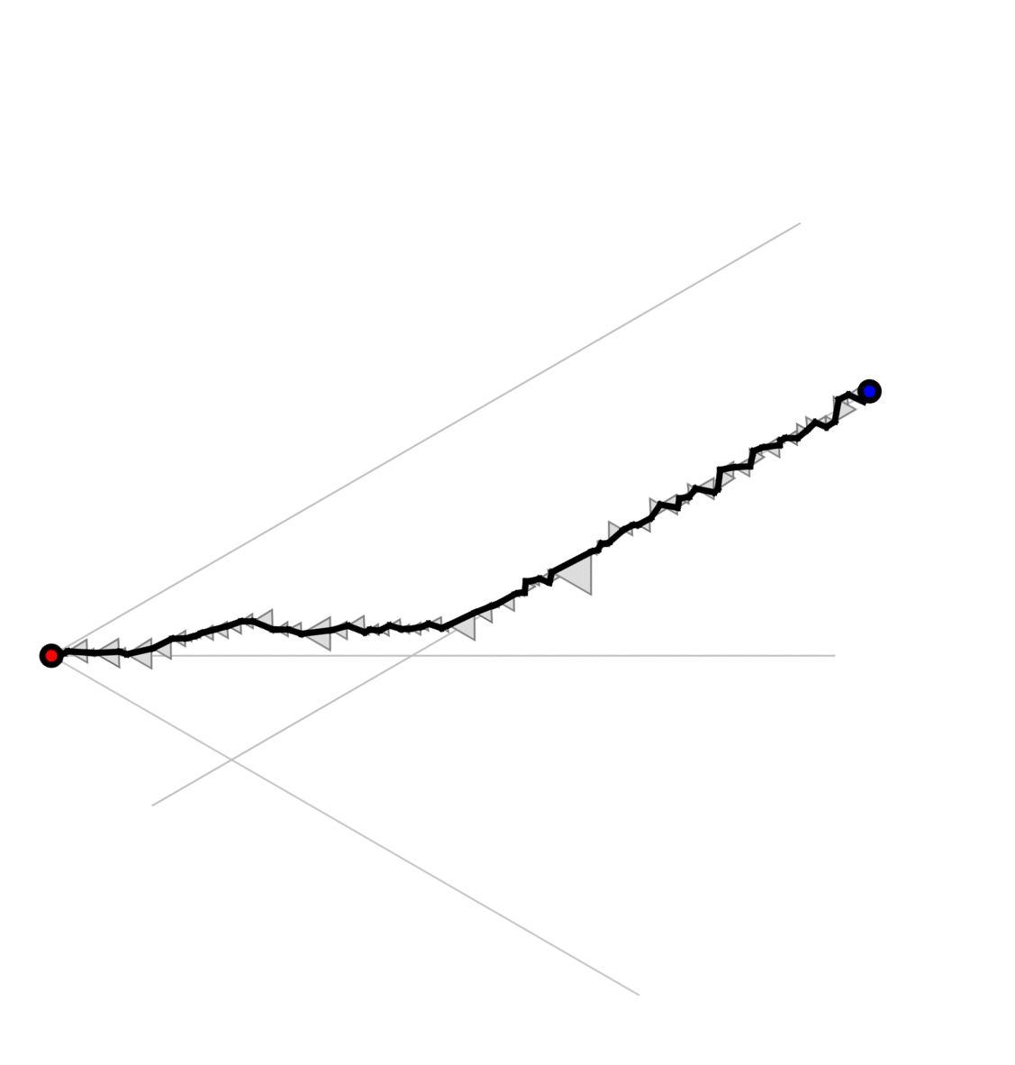
Figure 5: Examples of pθp_{\theta} CT navigation (for pθ=6p_{\theta}=6) with 500 nodes, 5000 nodes and 20000 nodes uniformly distributed in the unit square.

Again, for 𝐗∈{𝐂𝐓,𝐂𝐘}{\bf X}\in\{{\bf CT},{\bf CY}\}, the function x↦𝖯𝗈𝗌s,t𝐗(.n)x\mapsto{\sf Pos}_{s,t}^{{\bf X}}(.\sqrt{n}) admits a deterministic limit 𝖯𝗈𝗌s,t∞,a,b{\sf Pos}^{\infty,a,b}_{s,t} depending on two parameters aa and bb (which depend on 𝐗{\bf X} and θ\theta) related to the speed of the traveller along the two branches of Γ⁡(s,t)\Gamma(s,t). Set

𝖯𝗈𝗌s,t∞,λ,λ′​(x):={SOLsλ,arg⁡(I⁡(s,t)−s)⁡(x) for ​x∈[0,Times,I⁡(s,t)λ],SOLI⁡(s,t)λ′,arg⁡(t−I⁡(s,t))⁡(x−Times,I⁡(s,t)λ⁡(1)) if ​x∈Times,I⁡(s,t)λ+[0,TimeI⁡(s,t),tλ′],t if ​x≥Times,I⁡(s,t)λ+TimeI⁡(s,t),tλ′.{\sf Pos}^{\infty,\lambda,\lambda^{\prime}}_{s,t}(x):=\left\{\begin{array}[]{ll}\SOL_{s}^{\lambda,\arg(I(s,t)-s)}(x)&\textrm{ for }x\in[0,\Time_{s,I(s,t)}^{\lambda}],\\ \SOL_{I(s,t)}^{\lambda^{\prime},\arg(t-I(s,t))}(x-\Time_{s,I(s,t)}^{\lambda(1)})&\textrm{ if }x\in\Time_{s,I(s,t)}^{\lambda}+[0,\Time_{I(s,t),t}^{\lambda^{\prime}}],\\ t&\textrm{ if }x\geq\Time_{s,I(s,t)}^{\lambda}+\Time_{I(s,t),t}^{\lambda^{\prime}}.\end{array}\right. (10)
Theorem 6

Let 𝐗∈{𝐂𝐘,𝐂𝐓}{\bf X}\in\{{\bf CY},{\bf CT}\} and θ≤π/3\theta\leq\pi/3, for any α∈(0,1/8)\alpha\in(0,1/8), any β>0\beta>0, any nn large enough

ℙn​f​(sup(s,t)∈𝒟′​[a]supx≥0|𝖯𝗈𝗌s,t𝐗​(x​n)−𝖯𝗈𝗌s,t∞,𝐂𝐛𝐢𝐬𝐗,𝐂𝐛𝐨𝐫𝐗​(x)|≥n−α)≤n−β.\mathbb{P}_{nf}\left(\sup_{(s,t)\in{\cal D}^{\prime}[a]}\sup_{x\geq 0}\left|{\sf Pos}^{{\bf X}}_{s,t}(x\sqrt{n})-{\sf Pos}^{\infty,{\bf C_{bis}^{{\bf X}}},{\bf C_{bor}^{{\bf X}}}}_{s,t}(x)\right|\geq n^{-\alpha}\right)\leq n^{-\beta}.

As for the straight case, this entails the convergence for the Hausdorff distance of 𝖯𝖺𝗍𝗁⁡(s,t){\sf Path}(s,t) to Γ⁡(s,t)\Gamma(s,t).

Again, other results concerning other cost functions are studied in Section 4.2.

2.3 Extensions

The following extensions can be treated with the material available in the present paper. We just provide the main lines of their analysis.

2.3.1 Random north navigation

This is a version of the cross navigation where each point s∈Ss\in S has its own (random) north n⁡(s)n(s) used to compute 𝖢𝗋𝗈𝗌𝗌⁡(s){\sf Cross}(s). The random variables (n⁡(s),s∈S)(n(s),s\in S) are assumed to be i.i.d. and takes their values in [0,2​π][0,2\pi]. This can be used to model some imprecisions in the Yao’s construction, where the north is not exactly known22 2 Each distribution of n⁡(s)n(s) leads to a different behaviour for the traveller. If the value of n⁡(s)n(s) is 0 a.s., then this models coincides with the standard cross navigation. If the distribution of n⁡(s)n(s) owns several atoms, then the speed of the traveller may be different along numerous directions. by the points of SS. The corresponding navigation algorithm is defined as follows: A traveller at ss, choose the smallest integer κ\kappa in ⟦0,pθ−1⟧\llbracket 0,p_{\theta}-1\rrbracket such that tt lies in s+ei​n​(s)+i​k​θ​𝖲𝖾𝖼𝗍​(θ)s+e^{in(s)+ik\theta}{\sf Sect}(\theta) and consider the smallest rr such that s+ei​n​(s)+i​k​θ​𝖳𝗋𝗂​(θ)​(r)∩(S∪{t})s+e^{in(s)+ik\theta}{\sf Tri}(\theta)(r)\cap\left(S\cup\{t\}\right) is not empty. Then set 𝐑𝐍𝐓⁡(s,t)=z{\bf RNT}(s,t)=z, the element of this set with smallest argument.

Using the Camembert sections instead leads to the random north Yao’s navigation, 𝐑𝐍𝐘{\bf RNY}.

The uniform random north navigation is not much different to the straight one, the limiting path being segments, and the limiting path length being a multiple of the Euclidean distance. Using the same arguments than those given in the present paper, one can prove that the distance done by the traveller satisfies, for any θ≤π/3\theta\leq\pi/3, for any α∈(0,1/8)\alpha\in(0,1/8) and β>0\beta>0, if nn is large enough

ℙn​f​(sup(s,t)∈𝒟′​[a]|𝖯𝖺𝗍𝗁𝐗​(s,t)−𝐐𝐗​|s−t||≥n−α)≤n−β\mathbb{P}_{nf}\left(\sup_{(s,t)\in{\cal D}^{\prime}[a]}\left|{\sf Path}^{{\bf X}}(s,t)-{\bf Q}^{{\bf X}}|s-t|\right|\geq n^{-\alpha}\right)\leq n^{-\beta}

where

𝐐𝐑𝐍𝐓=θ/22​sin⁡(θ/2)​(1cos⁡(θ/2)+arcsinh⁡(tan⁡(θ/2))tan⁡(θ/2)),𝐐𝐑𝐍𝐘\displaystyle{\bf Q}^{{\bf RNT}}=\frac{\theta/2}{2\sin({\theta}/2)}\left(\frac{1}{\cos(\theta/2)}+\frac{\arcsinh(\tan(\theta/2))}{\tan(\theta/2)}\right),~~~{\bf Q}^{{\bf RNY}} =\displaystyle= θ22−2​cos⁡(θ).\displaystyle\frac{\theta^{2}}{2-2\cos(\theta)}.

The computation of these constants are done in Section 3.3.4; the proof of the globalisation of the bounds do not present any problem in this case.

2.3.2 Model of nn i.i.d. positions

Consider g∈Lip⋆⁡(𝒟)g\in\Lip^{\star}({\cal D}) such that 𝟙𝒟​g=1\mathbbm{1}_{{\cal D}}g=1. Let p1,…,pnp_{1},\dots,p_{n} be nn i.i.d. random points chosen in 𝒟{\cal D} under the distribution having gg as density. Set 𝐒gn:={p1,…,pn}{\bf S}^{n}_{g}:=\{p_{1},\dots,p_{n}\}, and by 𝐏gn{\bf P}^{n}_{g} the distribution of this set. The analysis of the navigations under ℙn​g\mathbb{P}_{ng} is simpler than under 𝐏gn{\bf P}^{n}_{g} since under ℙn​g\mathbb{P}_{ng} Markovian properties can be used; the derivation of the results under 𝐏gn{\bf P}^{n}_{g} will appear to be simple consequences of those on ℙn​g\mathbb{P}_{ng}. Indeed, the two models 𝐏gn{\bf P}_{g}^{n} and ℙn​g\mathbb{P}_{ng} are related via the classical fact

𝐏gn(.)=ℙn​g(.|#𝐒=n);{\bf P}_{g}^{n}(~.~)=\mathbb{P}_{ng}(~.~|\,\#{\bf S}=n); (11)

in other words 𝐊n​g{\bf K}_{ng} conditioned by #​𝐒​(n​g)=n\#{\bf S}(ng)=n has the same distribution as 𝐊gn{\bf K}_{g}^{n}.

For any measurable event AA (element of 𝒩\mathcal{N} as defined in Section 1.3) and any c>0c>0,

𝐏gn​(A)=ℙn​g​(A|#​𝐒=n)≤ℙn​g​(A)ℙn​g​(#​𝐒=n).{\bf P}_{g}^{n}(A)=\mathbb{P}_{ng}(A~|~\#{\bf S}=n)\leq\frac{\mathbb{P}_{ng}(A)}{\mathbb{P}_{ng}(\#{\bf S}=n)}.

Since #​𝐒​(n​g)\#{\bf S}(ng) is 𝖯𝗈𝗂𝗌𝗌𝗈𝗇⁡(n){\sf Poisson}(n) distributed, one sees that ℙn​g(#𝐒=n)≥c1n−1/2\mathbb{P}_{ng}(\#{\bf S}=n)\geq c_{1}n^{-1/2}, for nn large enough, for a constant c1>0c_{1}>0 (this is an application of the Stirling formula) and therefore

𝐏gn​(A)≤(1/c1)​n1/2​ℙn​g​(A),{\bf P}_{g}^{n}(A)\leq(1/c_{1})n^{1/2}\mathbb{P}_{ng}(A),

for nn large enough. All the results of the present paper under the form ℙn​g​(An)=o⁡(xn)\mathbb{P}_{ng}(A_{n})=o(x_{n}) for some decreasing function xnx_{n} can be transferred under 𝐏gn{\bf P}_{g}^{n} to the form 𝐏gn​(An)=O⁡(n1/2​ℙn​g​(An​g))=o⁡(n1/2​xn){\bf P}_{g}^{n}(A_{n})=O(n^{1/2}\mathbb{P}_{ng}(A_{ng}))=o(n^{1/2}x_{n}), that is a factor n1/2n^{1/2} on the bound must be added. Therefore, the main theorems of the present paper can be transferred to 𝐏gn{\bf P}_{g}^{n} without any problems since all results (or intermediate results) have the form ℙn​g​(An)=o⁡(xn)\mathbb{P}_{ng}(A_{n})=o(x_{n}) for xn=o(n−1/2)x_{n}=o(n^{-1/2}).

2.4 Link with other random objects

Refer to caption Refer to caption Refer to caption


Figure 6: Union of all paths (toward in a unique target) on 5000 uniform random points for: (a) a DT navigation with θ=2​π/7\theta=2\pi/7. (b) a SY navigation with θ=2​π/3\theta=2\pi/3. (c) a CT navigation with pθ=7p_{\theta}=7.

– In [5], the authors investigate a navigation 𝐍{\bf N} on a homogeneous PPP 𝐒{\bf S} on ℂ\mathbb{C}, where the traveller wants to reach the origin 0 of the plane: for a given ss, 𝐍⁡(s){\bf N}(s) is the closest element of ss in 𝐒∪{0}{\bf S}\cup\{0\}, which has the additional property to be closer to 0 than ss. Adding an edge between each s∈𝐒s\in{\bf S} and 𝐍⁡(s){\bf N}(s) one gets a tree, called the ‘‘radial spanning tree’’ of the PPP. 33 3 On the second picture in Fig.6 straight pθp_{\theta} Yao navigation with θ=2​π/3\theta=2\pi/3; this picture is quite similar to the Fig.1 in [5] even if the navigation is less homogeneous in that paper The authors provide numerous results concerning this tree; some local properties concerning the degree of the vertices, the length of edges, and some more global properties, as the behaviour of the subset of elements ss of 𝐒{\bf S} such that 𝐍⁡(s,k)=0{\bf N}(s,k)=0. In [8], the author goes on this study. Among other, functional along a path are studied (the tree has infinite number of ends, paths going to infinity).
– In [6, 16] the authors study the property of a so-called “minimal directed spanning tree” (MDST). To each finite subset SS of (0,1]2(0,1]^{2} is associated a tree as follows : x∈Sx\in S is connected by a directed edge to the nearest y∈S∪{(0,0)}y\in S\cup\{(0,0)\}, having both coordinates smaller. They then study the asymptotic total length of the MDST when SS follows various distributions, with |S|→+∞|S|\to+\infty.
– In [4], the authors examine a directed like navigation, where the set of points is a random subset of ℤd\mathbb{Z}^{d}: each point of this set is kept with probability p∈(0,1)p\in(0,1). They then examine the connectivity of the construction according to the dimension.
– Another object that may be related to directed navigation is the Brownian web. In [11], the authors construct a binary tree using as set of vertices the points of a homogeneous PPP in the plane. The parent-children relation is then induced by a kind of navigation, where, instead of Camembert section, a rectangle section is used; this is deeply similar to what is represented in picture 1 of Fig.6. They then show that in a certain sense, their object converges to the Brownian web (see the references therein for definitions and criteria of convergences to the Brownian web). What is done in the present paper concerning directed navigation let us conjecture that what is done in [11] could be extended to Yao’s graphs or Θ\Theta graphs associated to directed navigations. The main structural difference here is that the infinite tree constructed by directed navigation has an unbounded degree, when it was binary in [11].
– In a sequence of papers, Aldous and coauthors [1, 2, 3]… investigate numerous questions related to navigation (or traveller salesman type problem) in a PPP. In particular, in [1] sufficient conditions on navigation algorithms are given to have an asymptotic shape (where the shape is roughly, the set of points at distance smaller than rr to the origin, properly rescaled).

3 Toward the proofs, first considerations

3.1 Presentation of the analysis

We present here the main ideas used in the paper before entering into the details.

  • •

    Under ℙn​f\mathbb{P}_{nf}, a ball of radius rr included in 𝒟{\cal D} contains O⁡(n​r2)O(nr^{2}) point of 𝐒⁡(n​f){\bf S}(nf) in average, and with huge probability less than n1+ε​r2n^{1+\varepsilon}r^{2}, uniformly on all balls (Lemma 14). We restrict ourselves to the case where the navigation has the property to force the traveller to come closer to tt at each stage. Hence for a right r=rnr=r_{n}, Lemma 14 allows one to show that the contribution of the stages of the traveller in the final ball of radius rnr_{n} is negligible. See Section 3.5.

  • •

    To study the behaviour of the traveller far from its target, a local argument is used: under ℙn​f\mathbb{P}_{nf} for a non constant function ff, the stages (sj−sj−1,j≥1)(s_{j}-s_{j-1},j\geq 1) are not identically distributed, neither independent since the value of sj−1s_{j-1} affects the distribution of sj−sj−1s_{j}-s_{j-1}. But, if one considers only ana_{n} successive stages, with an→+∞a_{n}\to+\infty and an​nε/n→0a_{n}n^{\varepsilon}/\sqrt{n}\to 0, these stages stay in a small window around s0s_{0} with a huge probability; these stages appear moreover to roughly behave as i.i.d. random variables under the homogeneous PPP ℙn​f​(s0)\mathbb{P}_{nf(s_{0})}; the behavior of these ana_{n} stages are seen to depend at the first order, only of f⁡(s0)f(s_{0}). Moreover, since an→+∞a_{n}\to+\infty some regularizations of the type “law of large numbers” occur. See Section 3.3. This local theorem is one of the cornerstones of the study: in some sense, the global trajectory between any two points is a concatenation of these parts of length ana_{n}; the successive local values (f⁡(sk×an),k≥0)(f(s_{k\times a_{n}}),k\geq 0) yields directly to a differential equation. See section 3.4.

  • •

    The speed of convergence stated in the theorems is roughly given for each part of length ana_{n}: it is shown that well chosen deviations are exponential rare, and then the deviation between an entire trajectory and the limiting solution of the ODE is shown to have exponentially rare deviations. Hence, for free, this result maybe extended to all trajectories starting and ending on the two dimensional grid n−w​ℤ2∩𝒟n^{-w}\mathbb{Z}^{2}\cap{\cal D}, for some w>0w>0. The final globalisation consists in the comparison between the paths between any two points ss and tt of 𝒟{\cal D}, and some well chosen points of the grid n−w​ℤ2∩𝒟n^{-w}\mathbb{Z}^{2}\cap{\cal D}. This is possible if ww is large enough. See Section 4.3.

3.2 About the termination of the navigations

The main of this section is to state and prove the following proposition.

Proposition 7

Let 𝐗=𝐒𝐘{\bf X}={\bf SY} and θ≤2​π/3\theta\leq 2\pi/3, or 𝐗=𝐒𝐓{\bf X}={\bf ST} and θ≤π/2\theta\leq\pi/2, or 𝐗∈{𝐂𝐓,𝐂𝐘}{\bf X}\in\{{\bf CT},{\bf CY}\} and θ≤π/3\theta\leq\pi/3. Under ℙn​f\mathbb{P}_{nf}, a.s. for all (s,t)∈𝒟′​[a](s,t)\in{\cal D}^{\prime}[a]

  1. 1.

    the navigation from ss to tt succeeds (i.e. ∃k\exists k such that 𝐗⁡(s,t,k)=t{\bf X}(s,t,k)=t);

  2. 2.

    the traveller comes closer to the target at each step, 𝖯𝖺𝗍𝗁𝐗​(s,t)⊂B⁡(t,|s−t|){\sf Path}^{\bf X}(s,t)\subset B(t,|s-t|);

  3. 3.

    |𝖯𝖺𝗍𝗁𝐗​(s,t)|≤2​|s−t|×#​S∩B⁡(t,|s−t|)|{\sf Path}^{\bf X}(s,t)|\leq 2|s-t|\times\#S\cap B(t,|s-t|);

  4. 4.

    if |s1−s|≤|t−s|/2|s_{1}-s|\leq|t-s|/2 then |t−s|−|t−s1|≥(2−3)​|s1−s||t-s|-|t-s_{1}|\geq(2-\sqrt{3})|s_{1}-s|.

Proof. Let κ\kappa be the integer such that t∈𝖲𝖾𝖼𝗍⁡[κ,s]t\in{\sf Sect}[\kappa,s] and let tκt_{\kappa} be the orthogonal projection of tt on the bisecting line of the sector κ\kappa. Let 𝖠𝗋𝖾𝖺{\sf Area} be 𝖢𝖺𝗆​[κ,s]​(|s−t|){{\sf Cam}}[\kappa,s](|s-t|) (resp. 𝖳𝗋𝗂⁡[κ,s]​(|s−tκ|){{\sf Tri}}[\kappa,s](|s-t_{\kappa}|), 𝖢𝖺𝗆→​(s,t)​(|s−t|)\overrightarrow{{\sf Cam}}(s,t)(|s-t|) and 𝖳𝗋𝗂→​(s,t)​(|s−t|)\overrightarrow{{\sf Tri}}(s,t)(|s-t|)) if 𝐗{\bf X} is 𝐂𝐘{\bf CY} (resp. 𝐂𝐓{\bf CT}, 𝐒𝐘{\bf SY} and 𝐒𝐓{\bf ST}). For the values of θ\theta considered, 𝖠𝗋𝖾𝖺⊂B⁡(t,|s−t|){\sf Area}\subset B(t,|s-t|). In each case, s1∈𝖠𝗋𝖾𝖺s_{1}\in{\sf Area}, and so |s1−t|≤|s−t||s_{1}-t|\leq|s-t|, which implies the second item of the proposition. The previous inequality is strict except in one particular case for each navigation considered and only for the maximal values of θ\theta considered: in case 𝖠𝗋𝖾𝖺{\sf Area} contains only the two points tt and s1s_{1}, and s1s_{1} is on the first border of 𝖠𝗋𝖾𝖺{\sf Area} such that |s1−t|=|s−t||s_{1}-t|=|s-t|. Observe that in that case, arg⁡(s1−t)−arg⁡(s−t)\arg(s_{1}-t)-\arg(s-t) equals π/2\pi/2 if X=𝐒𝐓X={\bf ST} and π/3\pi/3 for the other navigations (still for the maximal values of θ\theta considered). Hence the navigation fails only if there exists (s,t)∈𝒟2(s,t)\in{\cal D}^{2} such that S∪{s}S\cup\{s\} contains 4 points (resp. 6 points) forming an empty square (resp. an empty hexagon) centred at tt with no other points of SS inside this polygon. Under ℙn​f\mathbb{P}_{nf}, almost surely SS doesn’t contain such a configuration. This implies the first item of the proposition.

The third item comes directly from the two first ones: the length of each stage of 𝖯𝖺𝗍𝗁𝐗​(s,t){\sf Path}^{\bf X}(s,t) is at most 2​|s−t|2|s-t| and 𝖯𝖺𝗍𝗁𝐗​(s,t){\sf Path}^{\bf X}(s,t) is composed of at most #​S∩B⁡(t,|s−t|)\#S\cap B(t,|s-t|) stages.

Now let us prove the last item. Let α:=arg⁡(t−s)−arg⁡(s1−s)\alpha:=\arg(t-s)-\arg(s_{1}-s). For the navigation considered, α∈[0,π/3]\alpha\in[0,\pi/3]. By the cosine law, we have:

|t−s1|2=|t−s|2+|s1−s|2−2​|t−s|.|s1−s|​cos⁡α.|t-s_{1}|^{2}=|t-s|^{2}+|s_{1}-s|^{2}-2|t-s|.|s_{1}-s|\cos\alpha. (12)

Let x≥2x\geq 2 such that |t−s|=x​|s1−s||t-s|=x|s_{1}-s|. By (12), |t−s1|=|s1−s|​x2+1−2​x​cos⁡α|t-s_{1}|=|s_{1}-s|\sqrt{x^{2}+1-2x\cos\alpha} and then |t−s|−|t−s1|=|s1−s|(x−x2+1−2​x​cos⁡α)|t-s|-|t-s_{1}|=|s_{1}-s|(x-\sqrt{x^{2}+1-2x\cos\alpha}). For x≥2x\geq 2, using that α↦cos⁡α\alpha\mapsto\cos\alpha is decreasing on [0,π/3][0,\pi/3], x−(x2+1−x)1/2≤x−x2+1−2​x​cos⁡α≤x−(x−1)x-(x^{2}+1-x)^{1/2}\leq x-\sqrt{x^{2}+1-2x\cos\alpha}\leq x-(x-1).Therefore (x−x2+1−2​x​cos⁡α)∈[2−3,1](x-\sqrt{x^{2}+1-2x\cos\alpha})\in[2-\sqrt{3},1], we get the last item. □\Box

3.3 A notion of directed navigation

In the straight navigation under ℙn​f\mathbb{P}_{nf}, when the traveller is far from its target, the fluctuations of arg⁡(t−si)\arg(t-s_{i}) stay small for the first values of ii (for large nn). It is then intuitive that the trajectory of the traveller would not be much changed if he’d use the constant direction given by arg⁡(t−s0)\arg(t-s_{0}) instead of arg⁡(t−si)\arg(t-s_{i}); similarly, in the cross navigation, when the traveller is far from 𝖢𝗋𝗈𝗌𝗌⁡(t){\sf Cross}(t), it is easily seen that along its first stages, the bisecting lines of its decision sectors are parallel to the first one, in other words, he follows the direction of the bisecting line of the sector around s0s_{0} containing tt. In order to make clear these phenomena, the directed navigation 𝐃𝐓{\bf DT} is defined below.

Again θ\theta is a fixed parameter chosen in (0,2​π)(0,2\pi).

Definition 8

∙\bullet 𝐃𝐓{\bf DT} is a map from ℂ\mathbb{C} onto SS defined as follows. Let s∈ℂs\in\mathbb{C}. If 𝖲𝖾𝖼𝗍→​(s,+∞)∩S\overrightarrow{{\sf Sect}}(s,+\infty)\cap S is empty, then 𝐃𝐓⁡(s){\bf DT}(s) is defined to be ss. Otherwise consider the smallest rr such that (s+𝖳𝗋𝗂​(θ)​(r))∩S\left(s+{\sf Tri}(\theta)(r)\right)\cap S is not empty. Then 𝐃𝐓⁡(s){\bf DT}(s) is defined to be the element of this intersection, that is the closest of the first border of 𝖲𝖾𝖼𝗍→​(s,+∞)\overrightarrow{{\sf Sect}}(s,+\infty).
∙\bullet
DYis defined similarly, except that (s+𝖢𝖺𝗆​(θ)​(r))∩S\left(s+{\sf Cam}(\theta)(r)\right)\cap S replaces (s+𝖳𝗋𝗂​(θ)​(r))∩S\left(s+{\sf Tri}(\theta)(r)\right)\cap S.

For any s∈ℂs\in\mathbb{C}, the successive stopping places (𝐃𝐓⁡(s,j),j≥0)({\bf DT}(s,j),j\geq 0) of the traveller satisfy 𝐃𝐓⁡(s,0)=s{\bf DT}(s,0)=s, 𝐃𝐓⁡(s,j)=𝐃𝐓⁡(𝐃𝐓⁡(s,j−1)){\bf DT}(s,j)={\bf DT}({\bf DT}(s,j-1)). Informally, DT coincides with ST if the target is t=+∞t=+\infty. If the directed navigation is done on a homogeneous PPP on ℂ\mathbb{C}, the stages

Δ𝐃𝐓​(s,j):=𝐃𝐓⁡(s,j)−𝐃𝐓⁡(s,j−1),j≥1\Delta^{{\bf DT}}(s,j):={\bf DT}(s,j)-{\bf DT}(s,j-1),~~~j\geq 1

are i.i.d.. Under ℙf\mathbb{P}_{f}, for a non constant ff, the process (𝐃𝐓⁡(s,j),j≥0)({\bf DT}(s,j),j\geq 0) is Markovian but the stages are not i.i.d.. (see the asymptotic behaviour of the directed navigation on Fig. 6(a)).

3.3.1 Directed navigation on a PPP with constant intensity

We consider now DT  under ℙc\mathbb{P}_{c} on all ℂ\mathbb{C}. We write the intensity in index position to let appear the rescaling arguments. Notice further that Δ𝐃𝐓​(s,j)\Delta^{{\bf DT}}(s,j) does not depend on ss; we then omit it. We remove now the superscript DT from everywhere. For any j≥1j\geq 1, write

Δc​(j)\displaystyle\Delta_{c}(j) =\displaystyle= xc​(j)+i​yc​(j)​for ​xc​(j),yc​(j)∈ℝ,\displaystyle x_{c}(j)+i\,y_{c}(j)~~~\textrm{for }x_{c}(j),y_{c}(j)\in\mathbb{R}, (13)

and set lc​(j)=|Δc​(j)|l_{c}(j)=\left|\Delta_{c}(j)\right|, the length of this stage. The stages (Δc​(j),j≥1)(\Delta_{c}(j),j\geq 1) are i.i.d., as well as the lengths (lc​(j),j≥1)(l_{c}(j),j\geq 1) and the pairs ((xc​(j),yc​(j)),j≥1)((x_{c}(j),y_{c}(j)),j\geq 1). By a clear space rescaling argument, we have the following equality in distribution for any j≥1j\geq 1,

Δc​(j)=(d)1c​Δ1​(j),(xc​(j),yc​(j))=(d)1c​(x1​(j),y1​(j)),lc​(j)=(d)1c​l1​(j).\Delta_{c}(j)\mathrel{\mathop{\kern 0.0pt=}\limits^{(d)}}\frac{1}{\sqrt{c}}\Delta_{1}(j),~~~~(x_{c}(j),y_{c}(j))\mathrel{\mathop{\kern 0.0pt=}\limits^{(d)}}\frac{1}{\sqrt{c}}(x_{1}(j),y_{1}(j)),~~~~l_{c}(j)\mathrel{\mathop{\kern 0.0pt=}\limits^{(d)}}\frac{1}{\sqrt{c}}l_{1}(j). (14)

Note x1x_{1} instead of x1​(1)x_{1}(1), y1y_{1} instead of y1​(1)y_{1}(1), etc. For any r>0r>0,

ℙ⁡(x1>r)\displaystyle\mathbb{P}(x_{1}>r) =\displaystyle= ℙ1​(#​𝖳𝗋𝗂​[κ,0]​(r)∩𝐒=0)=exp⁡(−r2​tan⁡(θ/2)),\displaystyle\mathbb{P}_{1}(\#{{\sf Tri}}[\kappa,0](r)\cap{\bf S}=0)=\exp\left(-r^{2}\tan(\theta/2)\right), (15)

and then, by integration, one finds 𝔼⁡(x1𝐃𝐓)=(1/2)​π/tan⁡(θ/2).\mathbb{E}(x_{1}^{{\bf DT}})=(1/2)\sqrt{{\pi}/{\tan(\theta/2)}}. Notice also that 𝔼⁡(x1𝐃𝐓)=𝐂𝐛𝐢𝐬𝐒𝐓=𝐂𝐛𝐢𝐬𝐂𝐓.\mathbb{E}(x_{1}^{{\bf DT}})={\bf C_{bis}^{{\bf ST}}}={\bf C_{bis}^{{\bf CT}}}. Now, since y1=x1​Uy_{1}=x_{1}U where UU is independent of x1x_{1} and uniform on [−tan⁡(θ2),tan⁡(θ2)]\left[-\tan(\frac{\theta}{2}),\tan(\frac{\theta}{2})\right],

l1=|Δ1|=x12+y12=x1​(1+tan2⁡(θ/2)​V2)1/2l_{1}=|\Delta_{1}|=\sqrt{x_{1}{}^{2}+y_{1}{}^{2}}=x_{1}\left(1+\tan^{2}(\theta/2)V^{2}\right)^{1/2}

for VV uniform in [0,1][0,1], independent of x1x_{1}. A trite computation leads to 𝔼⁡(1+tan2⁡(θ/2)​V2)=𝐐𝐛𝐢𝐬𝐒𝐓,\mathbb{E}\left(\sqrt{1+\tan^{2}(\theta/2)V^{2}}\right)={\bf Q_{bis}^{{\bf ST}}}, as given in the beginning of Section 2, and then 𝔼⁡(l1𝐃𝐓)=𝔼⁡(x1𝐃𝐓)×𝐐𝐛𝐢𝐬𝐒𝐓=𝐐𝐛𝐢𝐬𝐒𝐓​𝐂𝐛𝐢𝐬𝐒𝐓.\mathbb{E}(l_{1}^{{\bf DT}})=\mathbb{E}(x_{1}^{{\bf DT}})\times{\bf Q_{bis}^{{\bf ST}}}={\bf Q_{bis}^{{\bf ST}}}\ {\bf C_{bis}^{{\bf ST}}}. We consider another quantity that will play a special role during the analysis of cross navigation. Consider the coordinates (ξ1,ξ1′)(\xi_{1},\xi_{1}^{\prime}) of a stage Δ1\Delta_{1} in the coordinate system (0,e−iθ/2,e−iθ/2+iπ/2)(0,e^{-i\theta/2},e^{-i\theta/2+i\pi/2}):

Δ1=ξ1e−iθ/2+ξ1′e−iθ/2+iπ/2.\Delta_{1}=\xi_{1}e^{-i\theta/2}+\xi_{1}^{\prime}e^{-i\theta/2+i\pi/2}.

As seen on Fig. 7, ξ1\xi_{1} is the length of the projection of Δ1\Delta_{1} on HL0⁡(s)\HL_{0}(s).

Refer to caption


Figure 7: Representation of ξ1\xi_{1} and ξ1′\xi^{\prime}_{1}.

The middle of the projections of (x1,y1)(x_{1},y_{1}) and (x1,−y1)(x_{1},-y_{1}) coincides with the projection of (x1,0)(x_{1},0), and by symmetry of the law of y1y_{1},

𝔼⁡(ξ1𝐃𝐓)=𝔼⁡(x1𝐃𝐓)​cos⁡(θ/2)=𝐂𝐛𝐨𝐫𝐂𝐓.\mathbb{E}(\xi_{1}^{{\bf DT}})=\mathbb{E}(x_{1}^{{\bf DT}})\cos(\theta/2)={\bf C_{bor}^{{\bf CT}}}. (16)

Consider now the distance and the position of the traveller after kk stops

X1𝐃𝐓​(k)=∑j=1kx1𝐃𝐓​(j),Y1𝐃𝐓​(k)=∑j=1ky1𝐃𝐓​(j),L1𝐃𝐓​(k)=∑j=1kl1𝐃𝐓​(j),Ξ1𝐃𝐓​(k)=∑j=1kξ1𝐃𝐓​(j).X_{1}^{{\bf DT}}(k)=\sum_{j=1}^{k}x_{1}^{{\bf DT}}(j),~~~Y_{1}^{{\bf DT}}(k)=\sum_{j=1}^{k}y_{1}^{{\bf DT}}(j),~~~L_{1}^{{\bf DT}}(k)=\sum_{j=1}^{k}l_{1}^{{\bf DT}}(j),~~~\Xi_{1}^{{\bf DT}}(k)=\sum_{j=1}^{k}\xi_{1}^{{\bf DT}}(j).

By the law of large numbers, the following 4-tuple converges a.s.

(X1𝐃𝐓​(k)k,Y1𝐃𝐓​(k)k,L1𝐃𝐓​(k)k,Ξ1𝐃𝐓​(k)k)\displaystyle\left(\frac{X_{1}^{{\bf DT}}(k)}{k},\frac{Y_{1}^{{\bf DT}}(k)}{k},\frac{L_{1}^{{\bf DT}}(k)}{k},\frac{\Xi_{1}^{{\bf DT}}(k)}{k}\right) →𝑘a.s.\displaystyle\xrightarrow[k]{a.s.} (𝐂𝐛𝐢𝐬𝐂𝐓, 0,𝔼⁡(l1𝐃𝐓),𝐂𝐛𝐨𝐫𝐂𝐓)\displaystyle\left({\bf C_{bis}^{{\bf CT}}},\ 0,\ \mathbb{E}(l_{1}^{{\bf DT}}),\ {\bf C_{bor}^{{\bf CT}}}\right)

and also then, L1𝐃𝐓​(k)X1𝐃𝐓​(k)→𝑘a.s.𝔼⁡(l1𝐃𝐓)𝔼⁡(x1𝐃𝐓)=𝐐𝐛𝐢𝐬𝐒𝐓,\displaystyle\frac{L_{1}^{{\bf DT}}(k)}{X_{1}^{{\bf DT}}(k)}\xrightarrow[k]{a.s.}\frac{\mathbb{E}(l_{1}^{{\bf DT}})}{\mathbb{E}(x_{1}^{{\bf DT}})}={\bf Q_{bis}^{{\bf ST}}}, and Ξ1𝐃𝐓​(k)X1𝐃𝐓​(k)→𝑘a.s.𝔼⁡(l1𝐃𝐓)𝔼⁡(ξ1𝐃𝐓)=𝐐𝐛𝐨𝐫𝐂𝐓.\displaystyle\frac{\Xi_{1}^{{\bf DT}}(k)}{X_{1}^{{\bf DT}}(k)}\xrightarrow[k]{a.s.}\frac{\mathbb{E}(l_{1}^{{\bf DT}})}{\mathbb{E}(\xi_{1}^{{\bf DT}})}={\bf Q_{bor}^{{\bf CT}}}. These numbers are then the crucial coefficients appearing in Theorems 3 and 5.

3.3.2 Control of the fluctuations of X1𝐃𝐓​(k),Y1𝐃𝐓​(k)X_{1}^{{\bf DT}}(k),Y_{1}^{{\bf DT}}(k) and L1𝐃𝐓​(k)L_{1}^{{\bf DT}}(k)

First, it is easily checked that the random variables l1l_{1}, x1x_{1}, y1y_{1}, and ξ1\xi_{1} have exponential moments. Indeed, by (15), 𝔼⁡(et​|x1|)<+∞\mathbb{E}(e^{t|x_{1}|})<+\infty for any t>0t>0, and the other variables are controlled as follows: there exist some constants β,β′,β′′\beta,\beta^{\prime},\beta^{\prime\prime} (that depends only on θ\theta) such that

0≤|y1|≤β​x1,0≤l1≤β′​x1;0≤ξ1≤β′′​x1.0\leq|y_{1}|\leq\beta x_{1},0\leq l_{1}\leq\beta^{\prime}x_{1};0\leq\xi_{1}\leq\beta^{\prime\prime}x_{1}.

Therefore the variables |x1−𝔼⁡(x1)||x_{1}-\mathbb{E}(x_{1})|, |y1−𝔼⁡(y1)||y_{1}-\mathbb{E}(y_{1})| and |l1−𝔼⁡(l1)||l_{1}-\mathbb{E}(l_{1})|, |ξ1−𝔼⁡(ξ1)||\xi_{1}-\mathbb{E}(\xi_{1})| own also exponential moments, which permits to control the fluctuations of X1​(k),Y1​(k),L1​(k),Ξ1​(k)X_{1}(k),Y_{1}(k),L_{1}(k),\Xi_{1}(k) around their means by Petrov’s [17] Theorem 15 p.52, and Lemma 5 p.54 that we adapt a bit; if Zk=z1+⋯+zkZ_{k}=z_{1}+\dots+z_{k}, and the ziz_{i} are centred, have exponential moments (𝔼⁡(et​|z1|)<+∞\mathbb{E}(e^{t|z_{1}|})<+\infty, for some t>0t>0), then there exist constants α>0\alpha>0 and c>0c>0 such that

ℙ⁡(|Zm|≥x​m)≤2​exp⁡(−c​x2) if ​x≤α​mℙ⁡(|Zm|≥x​m)≤2​exp⁡(−c​x​m) if ​x≥α​m;\begin{array}[]{lllll}\mathbb{P}\left(\left|Z_{m}\right|\geq x\sqrt{m}\right)&\leq&2\exp(-c\,x^{2})&\textrm{~~~if }x\leq\alpha\sqrt{m}\\ \mathbb{P}\left(\left|Z_{m}\right|\geq x\sqrt{m}\right)&\leq&2\exp(-c\,x\sqrt{m})&\textrm{~~~if }x\geq\alpha\sqrt{m};\end{array} (17)

constants c,αc,\alpha depend only on the distribution of z1z_{1}, but not on mm (the same constant cc can be chosen for both bounds; we do this). A consequence is the following proposition.

Proposition 9

Let (xn)(x_{n}) be a sequence of real numbers such that xn→+∞x_{n}\to+\infty and xn=O⁡(n)x_{n}=O(\sqrt{n}). There exists a constant γ>0\gamma>0, such that for any mm large enough

ℙ(supk∈⟦1,m⟧|X1𝐃𝐓​(k)−k​𝔼​(x1𝐃𝐓)m|≥xm)≤2mexp(−γxm);\mathbb{P}\left(\sup_{k\in\llbracket 1,m\rrbracket}\left|\frac{X_{1}^{\bf DT}(k)-k\mathbb{E}(x_{1}^{\bf DT})}{\sqrt{m}}\right|\geq x_{m}\right)\leq 2m\exp(-\gamma x_{m});

The same results hold for Y1𝐃𝐓​(k)−k​𝔼​(y1𝐃𝐓)Y_{1}^{\bf DT}(k)-k\mathbb{E}(y_{1}^{\bf DT}), L1𝐃𝐓​(k)−k​𝔼​(l1𝐃𝐓)L_{1}^{\bf DT}(k)-k\mathbb{E}(l_{1}^{\bf DT}) and Ξ1𝐃𝐓​(k)−k​𝔼​(ξ1𝐃𝐓)\Xi_{1}^{\bf DT}(k)-k\mathbb{E}(\xi_{1}^{\bf DT}) and the same γ\gamma can be chosen for all the cases.

Proof.   The proofs for X1​(k),Y1​(k),L1​(k)X_{1}(k),Y_{1}(k),L_{1}(k) and Ξ1​(k)\Xi_{1}(k) are identical. For X1​(k)X_{1}(k), write

ℙ(supk∈⟦1,m⟧|X1​(k)−k​𝔼​(x1)m|≥xm)\displaystyle\mathbb{P}\left(\sup_{k\in\llbracket 1,m\rrbracket}\left|\frac{X_{1}(k)-k\mathbb{E}(x_{1})}{\sqrt{m}}\right|\geq x_{m}\right) ≤\displaystyle\leq ∑k=1mℙ⁡(|X1​(k)−k​𝔼​(x1)k|≥m1/2k​xm)\displaystyle\sum_{k=1}^{m}\mathbb{P}\left(\left|\frac{X_{1}(k)-k\mathbb{E}(x_{1})}{\sqrt{k}}\right|\geq\frac{m^{1/2}}{\sqrt{k}}x_{m}\right) (18)

then use the first or second bounds of (17) according to whether m1/2​xmk≤α​k\frac{m^{1/2}x_{m}}{\sqrt{k}}\leq\alpha\sqrt{k} or not. □\Box

Now, let (xn)(x_{n}) be a sequence of real numbers, such that xn→+∞x_{n}\to+\infty and xn=O⁡(n)x_{n}=O(\sqrt{n}). There exists γ>0\gamma>0, such that for any mm large enough

ℙ(supk∈⟦1,m⟧|X1𝐃𝐓​(k)+i​Y1𝐃𝐓​(k)−k​𝔼​(x1𝐃𝐓)m|≥xm)≤4mexp(−γxm).\mathbb{P}\left(\sup_{k\in\llbracket 1,m\rrbracket}\left|\frac{X_{1}^{\bf DT}(k)+iY_{1}^{\bf DT}(k)-k\mathbb{E}(x_{1}^{\bf DT})}{\sqrt{m}}\right|\geq x_{m}\right)\leq 4m\exp(-\gamma x_{m}). (19)

To see this, use Proposition 9 and that for uu and vv in ℝ\mathbb{R}, if |u+i​v|≥a|u+iv|\geq a then |u|≥a/2|u|\geq a/\sqrt{2} or |v|≥a/2|v|\geq a/\sqrt{2}.

In case the intensity of the PPP is constant and equal to c>0c>0, for any k≥1k\geq 1

Xc​(k)=d1c​X1​(k),Yc​(k)=d1c​Y1​(k),Lc​(k)=d1c​L1​(k)​Ξc​(k)=d1c​Ξ1​(k).X_{c}(k)\mathrel{\mathop{\kern 0.0pt=}\limits^{d}}\frac{1}{\sqrt{c}}X_{1}(k),~~~Y_{c}(k)\mathrel{\mathop{\kern 0.0pt=}\limits^{d}}\frac{1}{\sqrt{c}}Y_{1}(k),~~~L_{c}(k)\mathrel{\mathop{\kern 0.0pt=}\limits^{d}}\frac{1}{\sqrt{c}}L_{1}(k)~~~\Xi_{c}(k)\mathrel{\mathop{\kern 0.0pt=}\limits^{d}}\frac{1}{\sqrt{c}}\Xi_{1}(k). (20)

This allows one to transfer results obtained under ℙ1\mathbb{P}_{1} to ℙc\mathbb{P}_{c}, since for any Borelian AA in ℝk\mathbb{R}^{k},

ℙ⁡((X1​(1),…,X1​(k))∈A)\displaystyle\mathbb{P}((X_{1}(1),\dots,X_{1}(k))\in A) =\displaystyle= ℙ⁡((Xc​(1),…,Xc​(k))∈c​A).\displaystyle\mathbb{P}((X_{c}(1),\dots,X_{c}(k))\in\sqrt{c}A). (21)

3.3.3 Computations for directed pθp_{\theta} Yao navigation

We use the same notation as in the previous part; this time, for r>0r>0,

ℙ⁡(l1𝐃𝐘>r)\displaystyle\mathbb{P}\left(l_{1}^{{\bf DY}}>r\right) =\displaystyle= ℙ1(#𝖢𝖺𝗆[k,0](r)∩𝐒=0)=exp(−r2θ/2),\displaystyle\mathbb{P}_{1}(\#{{\sf Cam}}[k,0](r)\cap{\bf S}=0)=\exp\left(-r^{2}\theta/2\right), (22)

and x1𝐃𝐘=cos⁡(α)​l1𝐃𝐘x_{1}^{{\bf DY}}=\cos(\alpha)l_{1}^{{\bf DY}} and y1𝐃𝐘=sin⁡(α)​l1𝐃𝐘y_{1}^{{\bf DY}}=\sin(\alpha)l_{1}^{{\bf DY}} for a variable α\alpha uniform on [−θ/2,θ/2][-\theta/2,\theta/2], independent of l1𝐃𝐘l_{1}^{{\bf DY}}. Again, l1𝐃𝐘l_{1}^{{\bf DY}}, x1𝐃𝐘x_{1}^{{\bf DY}} and y1𝐃𝐘y_{1}^{{\bf DY}} own exponential moments, and on gets 𝔼⁡(y1𝐃𝐘)=0\mathbb{E}\left(y_{1}^{{\bf DY}}\right)=0 and

𝔼⁡(l1𝐃𝐘)=π2​θ,𝔼⁡(x1𝐃𝐘)=𝔼⁡(l1𝐃𝐘)​sin⁡(θ/2)θ/2=𝐂𝐛𝐢𝐬𝐒𝐘=𝐂𝐛𝐢𝐬𝐂𝐘.\mathbb{E}\left(l_{1}^{{\bf DY}}\right)=\sqrt{\frac{\pi}{2\theta}},~~~\mathbb{E}\left(x_{1}^{{\bf DY}}\right)=\mathbb{E}(l_{1}^{{\bf DY}})\frac{\sin(\theta/2)}{\theta/2}={\bf C_{bis}^{{\bf SY}}}={\bf C_{bis}^{{\bf CY}}}.

Moreover since ξ1𝐃𝐘=l1𝐃𝐘​cos⁡(θ/2+V)\xi_{1}^{{\bf DY}}=l_{1}^{{\bf DY}}\cos(\theta/2+V) where VV is uniform on [−θ/2,θ/2][-\theta/2,\theta/2] and independent of l1𝐃𝐘l_{1}^{{\bf DY}},

𝔼⁡(ξ1𝐃𝐘)\displaystyle\mathbb{E}(\xi_{1}^{{\bf DY}}) =\displaystyle= 𝔼⁡(l1𝐃𝐘)​∫−θ/2θ/2cos(α+θ/2)dαθ=𝔼⁡(l1𝐃𝐘)​sin⁡(θ)θ=𝐂𝐛𝐨𝐫𝐂𝐘\displaystyle\mathbb{E}(l_{1}^{{\bf DY}})\frac{\int_{-\theta/2}^{\theta/2}\cos(\alpha+\theta/2)d\alpha}{\theta}=\mathbb{E}(l_{1}^{{\bf DY}})\frac{\sin(\theta)}{\theta}={\bf C_{bor}^{{\bf CY}}}

and again, notice that 𝐐𝐛𝐨𝐫𝐂𝐘=𝔼⁡(l1𝐃𝐘)/𝔼⁡(ξ1𝐃𝐘){\bf Q_{bor}^{{\bf CY}}}=\mathbb{E}(l_{1}^{{\bf DY}})/\mathbb{E}(\xi_{1}^{{\bf DY}}), 𝐐𝐛𝐢𝐬𝐂𝐘=𝔼⁡(l1𝐃𝐘)/𝔼⁡(x1𝐃𝐘){\bf Q_{bis}^{{\bf CY}}}=\mathbb{E}(l_{1}^{{\bf DY}})/\mathbb{E}(x_{1}^{{\bf DY}}). This leads to

Proposition 10

In the DY case, we have

(L1𝐃𝐘​(k)k,X1𝐃𝐘​(k)k,Y1𝐃𝐘​(k)k,Ξ1𝐃𝐘​(k)k)\displaystyle\left(\frac{L_{1}^{{\bf DY}}(k)}{k},\frac{X_{1}^{{\bf DY}}(k)}{k},\frac{Y_{1}^{{\bf DY}}(k)}{k},\frac{\Xi_{1}^{{\bf DY}}(k)}{k}\right) →𝑘a.s.(𝔼⁡(l1𝐃𝐘),𝐂𝐛𝐢𝐬𝐂𝐘,0,𝐂𝐛𝐨𝐫𝐂𝐘),\displaystyle\xrightarrow[k]{a.s.}\left(\mathbb{E}(l_{1}^{{\bf DY}}),{\bf C_{bis}^{{\bf CY}}},0,{\bf C_{bor}^{{\bf CY}}}\right), (23)

and then L1𝐃𝐘​(k)X1𝐃𝐘​(k)→𝑘a.s.𝐐𝐛𝐢𝐬𝐂𝐘\displaystyle\frac{L_{1}^{{\bf DY}}(k)}{X_{1}^{{\bf DY}}(k)}\xrightarrow[k]{a.s.}{\bf Q_{bis}^{{\bf CY}}}, and L1𝐃𝐘​(k)Ξ1𝐃𝐘​(k)→𝑘a.s.𝐐𝐛𝐨𝐫𝐂𝐘.\displaystyle\frac{L_{1}^{{\bf DY}}(k)}{\Xi_{1}^{{\bf DY}}(k)}\xrightarrow[k]{a.s.}{\bf Q_{bor}^{{\bf CY}}}.

3.3.4 Computations for the random north model

We here consider the case where the n⁡(s)n(s) are i.i.d. uniform on [0,2​π][0,2\pi]. Let Δ𝐑𝐍𝐓\Delta^{{\bf RNT}} be the traveller stage (when going from ss to tt), and let x𝐑𝐍𝐓x^{{\bf RNT}} be the orthogonal projection of Δ𝐑𝐍𝐓\Delta^{{\bf RNT}} on the line (s,t)(s,t) and y𝐑𝐍𝐓y^{{\bf RNT}} that on the orthogonal of (s,t)(s,t). A simple computation gives 𝔼⁡(y1𝐑𝐍𝐓)=𝔼⁡(y1𝐑𝐍𝐘)=0\mathbb{E}\left(y_{1}^{{\bf RNT}}\right)=\mathbb{E}\left(y_{1}^{{\bf RNY}}\right)=0,

𝔼⁡(x1𝐑𝐍𝐓)\displaystyle\mathbb{E}\left(x_{1}^{{\bf RNT}}\right) =\displaystyle= 𝔼⁡(x1𝐃𝐓)​∫0θ/2cos⁡(ν)θ/2​𝑑ν=𝔼⁡(x1𝐃𝐓)​sin⁡(θ/2)θ/2,\displaystyle\mathbb{E}\left(x_{1}^{{\bf DT}}\right)\int_{0}^{\theta/2}\frac{\cos(\nu)}{\theta/2}\,d\nu=\mathbb{E}\left(x_{1}^{{\bf DT}}\right)\frac{\sin(\theta/2)}{\theta/2}, (24)
𝔼⁡(x1𝐑𝐍𝐘)\displaystyle\mathbb{E}\left(x_{1}^{{\bf RNY}}\right) =\displaystyle= 𝔼⁡(l1𝐃𝐘)​∫0θ∫0θcos⁡(ν−γ)θ2​𝑑ν​𝑑γ=𝔼⁡(l1𝐃𝐘)​2−2​cos⁡(θ)θ2.\displaystyle\mathbb{E}(l_{1}^{{\bf DY}})\int_{0}^{{\theta}}\int_{0}^{{\theta}}\frac{\cos(\nu-\gamma)}{\theta^{2}}\,d\nu\,d\gamma=\mathbb{E}(l_{1}^{{\bf DY}})\frac{2-2\cos(\theta)}{\theta^{2}}. (25)

The limiting quotients 𝐐𝐑𝐍𝐓{\bf Q}^{{\bf RNT}} and 𝐐𝐑𝐍𝐘{\bf Q}^{{\bf RNY}} are 𝐐𝐑𝐍𝐓=𝔼⁡(l1𝐃𝐓)𝔼⁡(x1𝐑𝐍𝐓)\displaystyle{\bf Q}^{{\bf RNT}}=\frac{\mathbb{E}(l_{1}^{{\bf DT}})}{\mathbb{E}(x_{1}^{{\bf RNT}})}, and 𝐐𝐑𝐍𝐘=𝔼⁡(l1𝐃𝐘)𝔼⁡(x1𝐑𝐍𝐘)\displaystyle{\bf Q}^{{\bf RNY}}=\frac{\mathbb{E}(l_{1}^{{\bf DY}})}{\mathbb{E}(x_{1}^{{\bf RNY}})}.

3.4 From local to global or why differential equations come into play

In Proposition 9 and in (19) a control of the difference between Xc𝐃𝐓​(k)X_{c}^{{\bf DT}}(k) and Yc𝐃𝐓​(k)Y_{c}^{{\bf DT}}(k) and their mean k​𝔼​(x1𝐃𝐓)/ck\mathbb{E}(x_{1}^{{\bf DT}})/\sqrt{c} and 0 is given. If the intensity is n​fnf, the “local intensity” around ss is n​f​(s)nf(s). Roughly, the first stages of the traveller starting from ss are close in distribution under ℙn​f\mathbb{P}_{nf} and under ℙn​f​(s)\mathbb{P}_{nf(s)}. Hence, at the first order, Xn​f𝐃𝐓​(k)X_{nf}^{{\bf DT}}(k) should be close to k​𝔼​(x1𝐃𝐓)/n​f​(s)k\mathbb{E}(x_{1}^{{\bf DT}})/\sqrt{nf(s)}: the speed of the traveller depends on the position, and therefore a differential equation appears.

To approximate 𝖯𝗈𝗌𝐃𝐓{\sf Pos}^{{\bf DT}} by the solution at a differential equation, we will split the traveller’s trajectory into some windows corresponding to some sequence of consecutive stages; the windows have to be small enough to keep the approximation of the local intensity n​fnf by n​f​(s)nf(s) to be relevant, and large enough to let the approximation Xn​f𝐃𝐓X_{nf}^{{\bf DT}} by k​𝔼​(x1𝐃𝐓)/n​f​(s)k\mathbb{E}(x_{1}^{{\bf DT}})/\sqrt{nf(s)} to be relevant too, that is large enough to let large number type compensations occur.

In this section, we present the tools related to the approximation of the traveller position by differential equations. Their proofs are postponed at the Appendix of the paper.

We start with some deterministic considerations. Consider DD an open subset of ℝd\mathbb{R}^{d} and let G:D→ℝdG:D\to\mathbb{R}^{d} a Lipschitz function. Denote by Eq⁡(G,z)\Eq(G,z) the following ordinary differential equation

Eq⁡(G,z):={y⁡(0)=z∈D,y′​(x)=G⁡(y⁡(x)), for ​x≥0.\Eq(G,z):=\left\{\begin{array}[]{rcl}y(0)&=&z\in D,\\ y^{\prime}(x)&=&G(y(x)),~~~~~\textrm{ for }x\geq 0.\end{array}\right. (26)

This class of equations contains the family of equations ODE\ODE defined in (8). By Cauchy-Lipschitz Theorem, Eq⁡(G,z)\Eq(G,z) admits a unique solution ys​o​l​(G,z)y_{sol(G,z)}, or more simply ysoly_{\sol} when no confusion on GG and zz is possible. This solution is defined on a maximal interval [0,λ⁡(G,z))[0,\lambda(G,z)), where λ⁡(G,z)\lambda(G,z) is the hitting time of the border of DD by ysoly_{\sol}.

Before giving a convergence criterion for random trajectories, here is a deterministic criterion very close to the so-called explicit Euler scheme convergence theorem.

Lemma 11

Let G:D→ℝdG:D\to\mathbb{R}^{d} be a Lipschitz function, z∈Dz\in D fixed, and λ∈[0,λ⁡(G,z))\lambda\in[0,\lambda(G,z)) given.

Let (an)(a_{n}) and (cn)(c_{n}) two sequences of positive real numbers going to 00, and (yn)(y_{n}) a sequence of continuous functions from [0,λ+an][0,\lambda+a_{n}] onto DD satisfying the following conditions:
𝑂𝑃𝐸𝑁a)a) yn​(0)=zy_{n}(0)=z for all n≥1n\geq 1,
𝑂𝑃𝐸𝑁b)b) for all n≥1n\geq 1, yny_{n} is linear between the points (jan,j∈⟦0,⌊λ/an⌋⟧)(ja_{n},j\in\llbracket 0,\lfloor\lambda/a_{n}\rfloor\rrbracket), and the slope of yny_{n} on these windows of size ana_{n} is well approximated by G∘ynG\circ y_{n} in the following sense:

supj=0,…,⌊λ/an⌋|yn​((j+1)​an)−yn​(j​an)an−G⁡(yn​(j​an))|≤cn\displaystyle\sup_{j=0,\dots,\lfloor\lambda/a_{n}\rfloor}\left|\frac{y_{n}\left((j+1)a_{n}\right)-y_{n}\left(ja_{n}\right)}{a_{n}}-G(y_{n}(ja_{n}))\right|\leq c_{n}

where we denote with an absolute value a norm in ℝd\mathbb{R}^{d}. Under these hypothesis, there exists Cλ>0C_{\lambda}>0, such that for nn large enough

supx∈[0,λ]|yn​(x)−ys​o​l​(G,z)​(x)|≤Cλ​max⁡{an,cn}.\sup_{x\in[0,\lambda]}\left|y_{n}(x)-y_{sol(G,z)}(x)\right|\leq C_{\lambda}\max\{a_{n},c_{n}\}.

Moreover, the constants CλC_{\lambda} can be chosen in such a way that the function λ↦Cλ\lambda\mapsto C_{\lambda} is bounded on all compact subsets of [0,λ⁡(G,z))[0,\lambda(G,z)) and does not depend on the initial condition z∈Dz\in D.

Note that we need yny_{n} to be defined on a slightly larger interval than [0,λ][0,\lambda] because of border effects.

We now extend this lemma to the convergence of a sequence of stochastic processes (𝐙n)({\bf Z}_{n}).

Corollary 12

Let G:D→ℝnG:D\to\mathbb{R}^{n} be a Lipschitz function, z∈Dz\in D fixed, and λ∈[0,λ⁡(G,z))\lambda\in[0,\lambda(G,z)) given.

Let (an)(a_{n}), (bn)(b_{n}), (cn)(c_{n}), (cn′)(c_{n}^{\prime}) and (dn)(d_{n}) be five sequences of positive real numbers going to 0; let (𝐙n)({\bf Z}_{n}) be a sequence of continuous stochastic processes from [0,λ+an][0,\lambda+a_{n}] onto DD satisfying the following conditions:
𝑂𝑃𝐸𝑁a)a) a.s. 𝐙n​(0)=z{\bf Z}_{n}(0)=z,
𝑂𝑃𝐸𝑁b)b) the slope of 𝐙n{\bf Z}_{n} on windows of size ana_{n} is well approximated by G∘𝐙nG\circ{\bf Z}_{n}, with a large probability:

supj∈⟦0,λ/an⟧ℙ(|𝐙n​((j+1)​an)−𝐙n​(j​an)an−G(𝐙n(jan))|≥cn)≤andn;\sup_{j\in\llbracket 0,\lambda/a_{n}\rrbracket}\mathbb{P}\left(\left|\frac{{\bf Z}_{n}\left((j+1)a_{n}\right)-{\bf Z}_{n}\left(ja_{n}\right)}{a_{n}}-G\left({\bf Z}_{n}(ja_{n})\right)\right|\geq c_{n}\right)\leq a_{n}d_{n}; (27)

OPENc)c) inside the windows, the fluctuations of 𝐙n{\bf Z}_{n} are small:

supj∈⟦0,λ/an⟧ℙ(supx∈[j​an,(j+1)​an]|𝐙n(x)−𝐙n(jan)−(x−jan)G(𝐙n(jan))|≥cn′)≤anbn.\sup_{j\in\llbracket 0,\lambda/a_{n}\rrbracket}\mathbb{P}\left(\sup_{x\in[ja_{n},(j+1)a_{n}]}\left|{\bf Z}_{n}\left(x\right)-{\bf Z}_{n}\left({ja_{n}}\right)-(x-ja_{n})G({\bf Z}_{n}(ja_{n}))\right|\geq c_{n}^{\prime}\right)\leq a_{n}b_{n}. (28)

If these three conditions are satisfied, then

ℙ⁡(supx∈[0,λ]|ys​o​l​(G,z)​(x)−𝐙n​(x)|≤Cλ​max⁡{an,cn,cn′})≥1−(λ+1)​(dn+bn)\mathbb{P}\left(\sup_{x\in[0,\lambda]}\left|y_{sol(G,z)}(x)-{\bf Z}_{n}(x)\right|\leq C_{\lambda}\max\{a_{n},c_{n},c_{n}^{\prime}\}\right)\geq 1-(\lambda+1)(d_{n}+b_{n})

for a function λ↦Cλ\lambda\mapsto C_{\lambda} independent of zz, bounded on every compact subsets of [0,λ⁡(G,z))[0,\lambda(G,z)).

Notice that condition (c)(c) contains (b)(b) if cn′≤cn​anc_{n}^{\prime}\leq c_{n}a_{n} which will be the case in the applications we have, but the present presentation allows one to better understand the underlying phenomenon.

3.5 On the largest stage and the maximum number of points in a ball

The following quantity

Navmax⁡[θ]​(S):=sups∈𝒟⁡[a],η∈[0,2​π]inf{h:#⁡(S∩(s+ei​η​𝖢𝖺𝗆​(θ)​(h)))≥1}\NAVMAX[\theta](S):=\sup_{s\in{\cal D}[a],\eta\in[0,2\pi]}\inf\left\{h:~\#\left(S\cap\left(s+e^{i\eta}{\sf Cam}(\theta)(h)\right)\right)\geq 1\right\}

is a bound on the largest stages length for all starting points (s∈𝒟⁡[a]s\in{\cal D}[a]) and targets (t∈𝒟t\in{\cal D}) and all navigations considered in this paper.

Lemma 13

For any θ∈(0,2​π]\theta\in(0,2\pi], any C>0C>0, if nn is large enough,

ℙn​f​(Navmax⁡[θ]≥nC−1/2)≤exp⁡(−nC/2).\mathbb{P}_{nf}\left(\NAVMAX[\theta]\geq n^{C-1/2}\right)\leq\exp\left(-n^{C/2}\right).

Proof. Consider a tiling of the plane with squares of size n−1/2+C/2n^{-1/2+C/2}. For nn large enough, each element of the family (s+ei​η𝖢𝖺𝗆(θ)(n−1/2+C),s∈ℂ,η∈[0,2π])(s+e^{i\eta}{\sf Cam}(\theta)(n^{-1/2+C}),s\in\mathbb{C},\eta\in[0,2\pi]) contains in its interior at least a square of the tiling. It suffices then to show that any square □\Box of the tiling intersecting 𝒟⁡[a]{\cal D}[a] intersects also 𝐒{\bf S}. But, ℙn​f(#S∩□=0)=exp(−∫□nf(z)dz)≤exp(−mfnC)\mathbb{P}_{nf}(\#S\cap\Box=0)=\exp(-\int_{\Box}nf(z)dz)\leq\exp(-m_{f}n^{C}) since n​f≥n​mfnf\geq nm_{f}, and the area of □\Box is n−1+Cn^{-1+C}. Since O⁡(n1−C)O(n^{1-C}) squares intersect the bounded domain 𝒟⁡[a]{\cal D}[a], by the union bound the probability that there exists a square containing no elements of 𝐒{\bf S} is O⁡(n1−C​exp⁡(−mf​nC))O(n^{1-C}\exp(-m_{f}n^{C})).  □\Box.

Now we turn our attention to

Maxball⁡[r]​(S):=max⁡{#⁡(S∩B⁡(x,r))|x∈𝒟⁡[a]},\MAXBALL[r](S):=\max\{\#(S\cap B(x,r))~|~x\in{\cal D}[a]\},

the maximum number of elements of SS in a ball with radius rr and having its centre in 𝒟⁡[a]{\cal D}[a].

Lemma 14

For any B>0B>0, ε>0\varepsilon>0, if nn is large enough

ℙn​f(Maxball[n−1/2+B]≥n2​B+ε)≤exp(−n2​B+ε).\mathbb{P}_{nf}\left(\MAXBALL\left[n^{-1/2+B}\right]\geq n^{2B+\varepsilon}\right)\leq\exp\left(-n^{2B+\varepsilon}\right).

Note that for s∈𝒟s\in{\cal D} the mean number of elements in B(s,n−1/2+B)∩𝐒(nf)B(s,n^{-1/2+B})\cap{\bf S}(nf) is O⁡(n2​B)O(n^{2B}).
Proof. Consider a tiling of the plane with squares of size an=nB−1/2a_{n}=n^{B-1/2}; denote by 𝖲𝗊𝗎a{\sf Squ}_{a} the subset of those having a distance to 𝒟⁡[a]{\cal D}[a] smaller than ana_{n}. Any disk B⁡(x,an)B(x,a_{n}) with x∈𝒟⁡[a]x\in{\cal D}[a] intersects a bounded number dd of such squares, with dd independent of BB. Hence for any positive sequence (bn)(b_{n}),

{Maxball[an](𝐒(nf))≥bn}⊂{sup□∈𝖲𝗊𝗎a#(𝐒(nf)∩□)≥bn/d}.\left\{\MAXBALL[a_{n}]({\bf S}(nf))\geq b_{n}\right\}\subset\left\{\sup_{\Box\in{\sf Squ}_{a}}\#\left({\bf S}(nf)\cap\Box\right)\geq b_{n}/d\right\}.

First #⁡(𝐒⁡(n​f)∩□)\#\left({\bf S}(nf)\cap\Box\right) is 𝖯𝗈𝗂𝗌𝗌𝗈𝗇⁡(∫□n​f​(u)​𝑑u){\sf Poisson}(\int_{\Box}nf(u)du) distributed, and ∫□n​f​(u)​𝑑u≤λ′:=∫□n​Mf​𝑑u=n​an2​Mf\int_{\Box}nf(u)du\leq\lambda^{\prime}:=\int_{\Box}nM_{f}du=na_{n}^{2}M_{f}. Secondly, for X∼𝖯𝗈𝗂𝗌𝗌𝗈𝗇⁡(λ)X\sim{\sf Poisson}(\lambda), and λ′>λ\lambda^{\prime}>\lambda, ℙ⁡(X≥r)=supt>0ℙ⁡(et​X≥et​r)≤supt>0e−t​r+λ′​(et−1).\mathbb{P}(X\geq r)=\sup_{t>0}\mathbb{P}(e^{tX}\geq e^{tr})\leq\sup_{t>0}e^{-tr+\lambda^{\prime}(e^{t}-1)}. By a simple (classical) optimisation on tt, one gets

ℙn​f​(#⁡(𝐒∩□)>bn/d)≤exp⁡(−bnd​ln⁡(bnd​n​an2​Mf)+bnd−n​an2​Mf).\mathbb{P}_{nf}\left(\#\left({\bf S}\cap\Box\right)>b_{n}/d\right)\leq\exp\left(-\frac{b_{n}}{d}\ln\left(\frac{b_{n}}{dna_{n}^{2}M_{f}}\right)+\frac{b_{n}}{d}-na_{n}^{2}M_{f}\right). (29)

To end, take an=n−1/2+Ba_{n}=n^{-1/2+B}, bn=n2​B+εb_{n}=n^{2B+\varepsilon} and apply the union bound to the O⁡(1/an2)O(1/a_{n}^{2}) squares of 𝖲𝗊𝗎a{\sf Squ}_{a}.□\hfill\square

For C>0,B>0,ε>0C>0,B>0,\varepsilon>0, consider the following events

Ω(n,C):={Navmax[θ]≤nC−1/2},Ωn,ε:={Maxball[nB−1/2]≤n(2+ε)​B}∩Ω(n,C).\Omega(n,C):=\left\{\NAVMAX[\theta]\leq n^{C-1/2}\right\},\Omega_{n,\varepsilon}:=\left\{\MAXBALL\left[n^{B-1/2}\right]\leq n^{(2+\varepsilon)B}\right\}\cap\Omega(n,C).

3.6 About the constants in the paper

The aim of this section is to discuss the role of the constants in this paper, and maybe to help the reader to follow more easily the computations.
– we will use nC−1/2n^{C-1/2} as a bound on Navmax\NAVMAX; this bound is valid with probability 1−exp⁡(−nC/2)1-\exp(-n^{C/2}), for nn large,
– the behaviour of the traveller close to its target is treated in Section 3.2. “Far to its target” (or to some particular points in the trajectory) means |t−s|≥nB−1/2|t-s|\geq n^{B-1/2}. When the traveller enters in the final ball B⁡(t,nB−1/2)B(t,n^{B-1/2}), he will make at most Maxball⁡[nB−1/2]\MAXBALL[n^{B-1/2}] additional stages to reach tt, that is at most n3​Bn^{3B} stages with probability 1−exp⁡(−n3​B)1-\exp(-n^{3B}).
– In Corollary 12, when the approximation by the solution of a differential equation is needed, a window with size ana_{n} arises. We will take

an=nw−1/2.a_{n}=n^{w-1/2}.

Taking into account the space normalisation, this corresponds to consider nwn^{w} stages of the traveller.

Some assumptions are made on the relative values of w,C,Bw,C,B (for example 2​w+3​C<1/22w+3C<1/2) in the statements of this paper. In any case, there is a choice of (w,C,B)(w,C,B) which fulfils all the requirements of all intermediate results, that is

0<w<1/4,2​w+3​C<1/2,C+w<B,0<B<1/4,C∈(0,1/2)0<w<1/4,~~2w+3C<1/2,~~C+w<B,~~0<B<1/4,~~C\in(0,1/2) (30)

as can easily be checked. Another quantity appearing later on is w′∈(0,1/2)w^{\prime}\in(0,1/2) related to the bound nαn^{\alpha}, α<1/8\alpha<1/8 appearing in the paper in most of the important theorems. This α\alpha appears to be max⁡{w⁡(w′−1/2),w⁡(w′+1/2)−1/2,w−1/2}\max\{w(w^{\prime}-1/2),w(w^{\prime}+1/2)-1/2,w-1/2\} where (w,C,B,w′)(w,C,B,w^{\prime}). To reach an α\alpha close to (1/8)−(1/8)^{-}, take w=(1/4)−w=(1/4)^{-}, C=0+C=0^{+}, B=(1/4)−B=(1/4)^{-}, w′=0+w^{\prime}=0^{+}.

3.7 Navigations in homogeneous / non homogeneous PPP

Here is defined the notion of simple stages, notion related to non-intersecting decision domains.

Definition 15

Let (d1,…,dk)(d_{1},\dots,d_{k}) be the kk first stages of a traveller going from ss to tt. We say that these stages are 𝐗⁡(s,t)\Nav(s,t)-simple if the corresponding decision domains do not intersect; this amounts to saying that if the traveller uses as set of possible stops {s+∑j=1idi,i≤k}\{s+\sum_{j=1}^{i}d_{i},~i\leq k\}, then the decision sectors are non intersecting when going from ss to tt (see Fig. 8). A Borelian subset Θ\Theta of ℂk\mathbb{C}^{k} is said to be 𝐗⁡(s,t)\Nav(s,t)-simple if for any sequence (d1,…,dk)∈Θ(d_{1},\dots,d_{k})\in\Theta, the stages (d1,…,dk)(d_{1},\dots,d_{k}) are 𝐗⁡(s,t)\Nav(s,t)-simple.

Refer to caption


Figure 8: Example of configuration of points in the straight Yao navigation leading to an intersection of the decision domains. For DT the decision sectors are simple for θ≤π\theta\leq\pi, and for 𝐃𝐘{\bf DY}, the condition is θ≤π/2\theta\leq\pi/2. For 𝐒𝐓{\bf ST} and 𝐒𝐘{\bf SY}, for any θ\theta, the decision sectors can intersect.

Next proposition is really important. It provides around a point ss, a bound of the deviations of the traveller stages under the non homogeneous ℙn​f\mathbb{P}_{nf} using the much simpler measure ℙn​f​(s)\mathbb{P}_{nf(s)}. We were unable to find a sufficient coupling argument; this is a comparison of distributions.

Let us set the following vectorial notation:

Δ𝐃𝐓​[s,j]\displaystyle\Delta^{{\bf DT}}[s,j] :⁣=\displaystyle:= (Δ𝐃𝐓​(s,1),…,Δ𝐃𝐓​(s,j));\displaystyle\left(\Delta^{{\bf DT}}(s,1),\dots,\Delta^{{\bf DT}}(s,j)\right);

in the sequel, Δ𝐗​[s,t,j]\Delta^{{\bf X}}[s,t,j] and other similar notation will be used for the other navigation processes 𝐗\Nav if the target is needed to be specified.

Proposition 16

Let 𝐗∈{𝐂𝐘,𝐂𝐓}{\bf X}\in\{{\bf CY},{\bf CT}\} and θ≤π/3\theta\leq\pi/3, or 𝐗=𝐒𝐘{\bf X}={\bf SY} and θ<π/2\theta<\pi/2, or 𝐗=𝐒𝐓{\bf X}={\bf ST} and θ≤π/2\theta\leq\pi/2, or 𝐗=𝐃𝐓{\bf X}={\bf DT} and θ≤π\theta\leq\pi, or 𝐗=𝐃𝐘{\bf X}={\bf DY} and θ≤π/2\theta\leq\pi/2. Assume that (γn)(\gamma_{n}) is a sequence of integers such that γn∼nw\gamma_{n}\sim n^{w} for some w∈(0,1/4)w\in(0,1/4). Let C∈(0,1/2)C\in(0,1/2) such that 2​w+3​C<1/22w+3C<1/2, and (s,t)∈𝒟′​[a](s,t)\in{\cal D}^{\prime}[a]. For any Θ\Theta Borelian subset of ℂγn\mathbb{C}^{\gamma_{n}} 𝐗⁡(s,t){\bf X}(s,t)-simple, for nn large enough

ℙn​f​(Δ𝐗​[s,t,γn]∈Θ)≤exp⁡(−nC/2)+2​ℙn​f​(s)​(Δ𝐗​[s,t,γn]∈Θ),\mathbb{P}_{nf}\left(\Delta^{{\bf X}}[s,t,\gamma_{n}]\in\Theta\right)\leq\exp(-n^{C/2})+2\ \mathbb{P}_{nf(s)}\left(\Delta^{{\bf X}}[s,t,\gamma_{n}]\in\Theta\right),

where “tt” has to be omitted if 𝐗∈{𝐃𝐓,𝐃𝐘}{\bf X}\in\{{\bf DT},{\bf DY}\}, since the target does not exist in this case.

This proposition discusses a very local property since after nwn^{w} steps the traveller is with great probability at distance nw+C−1/2<<1n^{w+C-1/2}<<1 of its starting point, and then still in 𝒟{\cal D} for nn large.

This proposition permits to see that an event with small probability under ℙn​f​(s)\mathbb{P}_{nf(s)} (as to observe a large value for ∑i=1γnΔ𝐃𝐓​(s,i)−𝔼⁡(∑i=1γnΔ𝐃𝐓​(s,i))\sum_{i=1}^{\gamma_{n}}\Delta^{{\bf DT}}(s,i)-\mathbb{E}(\sum_{i=1}^{\gamma_{n}}\Delta^{{\bf DT}}(s,i)) as says Proposition 9) is also small under ℙn​f\mathbb{P}_{nf}.

Remark 17

The simplicity of the stages is unlikely to arise when ss is close to tt since the decision domains loose the property to have “a constant” direction. For this reason, this proposition will be used only when ss is far from tt. Notice also that the factor 2 in the RHS is taken for convenience, any number greater than 1 also does the job.

Proof of Proposition 16. By Lemma 13, for nn large, ℙn​f​(∁​Ω​(n,C))≤exp⁡(−nC/2)\mathbb{P}_{nf}(\complement\Omega(n,C))\leq\exp(-n^{C/2}). Write

ℙn​f​(Δ𝐗​[s,t,γn]∈Θ)≤ℙn​f​(∁​Ω​(n,C))+ℙn​f​(Δ𝐗​[s,t,γn]∈Θ,Ω⁡(n,C)).\mathbb{P}_{nf}(\Delta^{{\bf X}}[s,t,\gamma_{n}]\in\Theta)\leq\mathbb{P}_{nf}(\complement\Omega(n,C))+\mathbb{P}_{nf}(\Delta^{{\bf X}}[s,t,\gamma_{n}]\in\Theta,\Omega(n,C)).

We then just have to bound the second term in the RHS. For this, we will show that

ℙn​f​(Δ𝐗​[s,t,γn]∈Θ,Ω⁡(n,C))\displaystyle\mathbb{P}_{nf}(\Delta^{{\bf X}}[s,t,\gamma_{n}]\in\Theta,\Omega(n,C)) ≤\displaystyle\leq 2​ℙn​f​(s)​(Δ𝐗​[s,t,γn]∈Θ,Ω⁡(n,C))≤2​ℙn​f​(s)​(Δ𝐗​[s,t,γn]∈Θ),\displaystyle 2\,\mathbb{P}_{nf(s)}(\Delta^{{\bf X}}[s,t,\gamma_{n}]\in\Theta,\Omega(n,C))\leq 2\,\mathbb{P}_{nf(s)}(\Delta^{{\bf X}}[s,t,\gamma_{n}]\in\Theta),

only the first inequality deserving to be proved. We will show more; it is easy to see that under ℙn​f\mathbb{P}_{nf} and under ℙn​f​(s)\mathbb{P}_{nf(s)}, the distribution of Δ𝐗​[s,γn]\Delta^{{\bf X}}[s,\gamma_{n}] owns a density with respect to the Lebesgue measure on ℂγn\mathbb{C}^{\gamma_{n}}, that we denote by 𝐃1{\bf D}_{1} and 𝐃2{\bf D}_{2}, respectively44 4 more exactly, the representation of the probability measure of Δ𝐗​[s,γn]\Delta^{{\bf X}}[s,\gamma_{n}] using densities holds when small stages are considered, small enough such that all decision sectors considered are included in 𝒟{\cal D}, and small enough such that the target is not reached after the γn\gamma_{n} first steps. We will then compare these densities, and bound their ratio on a set of interest.

Since the distribution of the stages depend on decision sectors that have a shape depending on 𝐗{\bf X}, it is useful here to introduce some notation. Denote by d𝐗​(s,t)d^{\bf X}(s,t) the decision domain (a Camembert section or a triangular domain) corresponding to Δ​(s,t)𝐗\Delta(s,t)^{\bf X}, and by ∂d𝐗​(s,t)\partial{d}^{\bf X}(s,t) the corresponding principal boundaries, namely, depending on 𝐗{\bf X}, the side of the triangle which is not on the decision sector, and the arc of circle in the Camembert section. We write with an absolute value the Lebesgue measures of these sets. Let finally 𝖲𝖾𝗀𝐗​(s,t){\sf Seg}^{\bf X}(s,t) be the length of the segment of the plane starting from ss, supported by the bisecting line of the decision sector, and whose second end is on ∂d𝐗​(s,t)\partial{d}^{\bf X}(s,t).

Under ℙn​f\mathbb{P}_{nf} (resp. ℙn​f​(s)\mathbb{P}_{nf(s)}), conditionally on ∂d𝐗​(s,t)\partial{d}^{\bf X}(s,t), the density of the law of Δ𝐗​(s,t)\Delta^{\bf X}(s,t) is proportional to nf(s+.)nf(s+.) (resp. is uniform) on ∂d𝐗​(s,t)\partial{d}^{\bf X}(s,t). To characterise the law of Δ𝐗​(s,t)\Delta^{\bf X}(s,t) it remains to express the distribution of |𝖲𝖾𝗀𝐗​(s,t)||{\sf Seg}^{\bf X}(s,t)|; this latter is characterised by the following:

ℙn​f(|𝖲𝖾𝗀X(s,t)|>x)=exp(−∫d𝐗​(s,t,x)nf(u)du),\mathbb{P}_{nf}(|{\sf Seg}^{X}(s,t)|>x)=\exp\left(-\int_{d^{\bf X}(s,t,x)}nf(u)du\right),

where d𝐗​(s,t,x)d^{\bf X}(s,t,x) is the decision domain such that |𝖲𝖾𝗀𝐗​(s,t)|=x|{\sf Seg}^{\bf X}(s,t)|=x. The density of |𝖲𝖾𝗀𝐗​(s,t)||{\sf Seg}^{\bf X}(s,t)| is then

(∫∂d𝐗​(s,t,x)nf(u)du)exp(−∫d𝐗​(s,t,x)nf(u)du);\left(\int_{\partial d^{\bf X}(s,t,x)}nf(u)du\right)\exp\left(-\int_{d^{\bf X}(s,t,x)}nf(u)du\right);

The density of the same variable under ℙn​f​(s)\mathbb{P}_{nf(s)} is obtained by replacing f⁡(u)f(u) by the constant value f⁡(s)f(s) in this formula. Finally, under ℙn​f\mathbb{P}_{nf} the density of Δ𝐗​(s,t)\Delta^{\bf X}(s,t) is

gn​f,s,t(δ)=f(s+δ)exp(−∫d𝐗​(s,t,x​(δ))nf(u)du)g_{nf,s,t}(\delta)=f(s+\delta)\exp\left(-\int_{d^{\bf X}(s,t,x(\delta))}nf(u)du\right) (31)

for any δ\delta in the decision sector of the traveller going from ss to tt using 𝐗{\bf X}, where x⁡(δ)x(\delta) is the length of |𝖲𝖾𝗀𝐗​(s,t)||{\sf Seg}^{\bf X}(s,t)| corresponding to the stage δ\delta (again, this holds for “small stages”); under ℙn​f​(s)\mathbb{P}_{nf(s)} it is

gn​f​(s),s,t(δ)=f(s)exp(−∫d𝐗​(s,t,x​(δ))nf(s)du)g_{nf(s),s,t}(\delta)=f(s)\exp\left(-\int_{d^{\bf X}(s,t,x(\delta))}nf(s)du\right) (32)

where this last integral value is nf(s)|d𝐗(s,t,x)|=nf(s)|d𝐗(.,.,x)|nf(s)|d^{\bf X}(s,t,x)|=nf(s)|d^{\bf X}(.,.,x)|. Now, let us treat several stages 𝗏:=(δ1,…,δγn)∈Θ{\sf v}:=(\delta_{1},\dots,\delta_{\gamma_{n}})\in\Theta. We will use two ingredients. First the simplicity of Θ\Theta which guaranties the non intersection of the decision domains; this let us use formulas as (31) and (32), successively. Under the non intersecting condition by successively conditioning on the first stages of the traveller it appears that 𝐃1{\bf D}_{1} and 𝐃2{\bf D}_{2} have a multiplicative form:

𝐃1​(𝗏)\displaystyle{\bf D}_{1}({\sf v}) =\displaystyle= ∏i=1γngn​f​(s),si−1,t​(δi),𝐃2​(𝗏)=∏i=1γngn​f,si−1,t​(δi)\displaystyle\prod_{i=1}^{\gamma_{n}}g_{nf(s),s_{i-1},t}(\delta_{i}),~~{\bf D}_{2}({\sf v})=\prod_{i=1}^{\gamma_{n}}g_{nf,s_{i-1},t}(\delta_{i}) (33)

where s0=ss_{0}=s, sj=s0+δ1+⋯+δjs_{j}=s_{0}+\delta_{1}+\dots+\delta_{j}. The sequence (d𝐗​(si,t,x⁡(δi)),i=1,…,γn)(d^{\bf X}(s_{i},t,x(\delta_{i})),i=1,\dots,\gamma_{n}) appearing is the same in both formulas, and then 𝐃1{\bf D}_{1} and 𝐃2{\bf D}_{2} are very similar. Let us see why 𝐃2​(𝗏)≤2​𝐃1​(𝗏){\bf D}_{2}({\sf v})\leq 2{\bf D}_{1}({\sf v}) holds for any element 𝗏{\sf v} in Ω⁡(n,C)∩Θ\Omega(n,C)\cap\Theta which will be enough to conclude.

For this, consider the first factor ∏i=1γnf⁡(si−1+δi)\prod_{i=1}^{\gamma_{n}}f(s_{i-1}+\delta_{i}) appearing in 𝐃2{\bf D}_{2}. If 𝗏∈Ω⁡(n,C){\sf v}\in\Omega(n,C), for m≤γnm\leq\gamma_{n}, since ff is Lipschitzian,

∏i=1γnf⁡(si−1+δi)≤∏i=1γnf⁡(s)+αf​γn​nC−1/2≤f​(s)γn​(1+c1​γn​nC−1/2)γn,\prod_{i=1}^{\gamma_{n}}f(s_{i-1}+\delta_{i})\leq\prod_{i=1}^{\gamma_{n}}f(s)+\alpha_{f}\,\gamma_{n}n^{C-1/2}\leq f(s)^{\gamma_{n}}(1+c_{1}\gamma_{n}n^{C-1/2})^{\gamma_{n}},

for constants c1>0c_{1}>0 and αf\alpha_{f}, since ff is bounded. Let us bound the second factor appearing in 𝐃2{\bf D}_{2} :

exp(−n∫d𝐗​(sm−1,t,δm)f(u)du)\displaystyle\exp\left(-n\int_{d^{\bf X}(s_{m-1},t,\delta_{m})}f(u)du\right) =\displaystyle= exp(−n∫d𝐗​(sm−1,t,δm)f(u)−f(s)du)\displaystyle\exp\left(-n\int_{d^{\bf X}(s_{m-1},t,\delta_{m})}f(u)-f(s)du\right) (35)
×exp(−n∫d𝐗​(sm−1,t,δm)f(s)du)\displaystyle\times\exp\left(-n\int_{d^{\bf X}(s_{m-1},t,\delta_{m})}f(s)du\right)

the second term of this product is simply exp⁡(−n​f​(s)​|d𝐗​(sm−1,t,δm)|)\exp\left(-nf(s)|d^{\bf X}(s_{m-1},t,\delta_{m})|\right); let us bound the first one. Using that the area of d𝐗​(sm−1,t,δm)d^{\bf X}(s_{m-1},t,\delta_{m}) is bounded by c2​n2​C−1c_{2}n^{2C-1} (since δm≤nC−1/2\delta_{m}\leq n^{C-1/2}), and that f⁡(u)−f⁡(s)f(u)-f(s) is greater than −αf​m​nC−1/2-\alpha_{f}mn^{C-1/2} (Lipschitz, and since we are in Ω⁡(n,C)\Omega(n,C), |t−s|≤m​nC−1/2|t-s|\leq m\,n^{C-1/2}), we get that the LHS of (35) is bounded by

exp(−n∫d𝐗​(sm−1,t,δm)f(u)−f(s)du)\displaystyle\exp\left(-n\int_{d^{\bf X}(s_{m-1},t,\delta_{m})}f(u)-f(s)du\right) ≤\displaystyle\leq exp⁡(c2​n×m​nC−1/2​n2​C−1)=exp⁡(c2​m​n3​C−1/2)\displaystyle\exp\left(c_{2}n\times mn^{C-1/2}n^{2C-1}\right)=\exp(c_{2}\,m\,n^{3C-1/2})

for some constant c2>0c_{2}>0. Finally, putting together the γn\gamma_{n} terms involved,

𝐃2​(𝗏)≤𝐃1​(v)×(1+c1​γn​nC−1/2)γn×∏m=1γnexp⁡(c2​m​n3​C−1/2).{\bf D}_{2}({\sf v})\leq{\bf D}_{1}(v)\times\left(1+c_{1}\gamma_{n}n^{C-1/2}\right)^{\gamma_{n}}\times\prod_{m=1}^{\gamma_{n}}\exp\left(c_{2}mn^{3C-1/2}\right). (36)

Recall that γn∼nw→+∞\gamma_{n}\sim n^{w}\to+\infty. The first term (1+c1​γn​nC−1/2)γn(1+c_{1}\gamma_{n}n^{C-1/2})^{\gamma_{n}} goes to 1 if C<1/2C<1/2. The second term goes to 1 if ∑m=1γnc2​m​n3​C−1/2\sum_{m=1}^{\gamma_{n}}c_{2}mn^{3C-1/2} goes to 0, that is if 2​w+3​C−1/2<02w+3C-1/2<0. Finally, taking C∈(0,1/2)C\in(0,1/2) and w>0w>0 satisfying 2​w+3​C−1/2<02w+3C-1/2<0, we see that (1+c1​γn​nC−1/2)γn×∏m=1γnexp⁡(c2​m​n3​C−1/2)→1\left(1+c_{1}\gamma_{n}n^{C-1/2}\right)^{\gamma_{n}}\times\prod_{m=1}^{\gamma_{n}}\exp\left(c_{2}mn^{3C-1/2}\right)\to 1, and thus is less than 22 for nn large enough. □\hfill\square

3.8 Limiting behaviour for a traveller using DT or DY

In this section, we deal with DT, but DY can be studied similarly. The aim is to show that when n→+∞n\to+\infty, after rescaling, the function 𝖯𝗈𝗌s𝐃𝐓{\sf Pos}_{s}^{{\bf DT}} under ℙn​f\mathbb{P}_{nf} converges in distribution to SOLs𝐂𝐛𝐢𝐬𝐂𝐓,0\SOL_{s}^{{\bf C_{bis}^{{\bf CT}}},0} the solution of ODE⁡(𝐂𝐛𝐢𝐬𝐂𝐓,0,s)\ODE({\bf C_{bis}^{{\bf CT}}},0,s) as defined in (8).

Theorem 18

Let 𝐗=𝐃𝐓{\bf X}={\bf DT} and θ≤π\theta\leq\pi or 𝐗=𝐃𝐘{\bf X}={\bf DY} and θ≤π/2\theta\leq\pi/2. For any s∈𝒟⁡[a]s\in{\cal D}[a], any α∈(0,1/8)\alpha\in(0,1/8), for λ∈[0,λ⁡(F𝐂𝐛𝐢𝐬𝐗,0,s))\lambda\in[0,\lambda(F_{{\bf C_{bis}^{{\bf X}}},0},s)), there exists a constant d>0d>0 such that for nn large enough

ℙn​f​(supx∈[0,λ]|𝖯𝗈𝗌s𝐃𝐓​(x​n)−SOLs𝐂𝐛𝐢𝐬𝐂𝐓,0⁡(x)|≤n−α)≥1−exp⁡(−nd).\mathbb{P}_{nf}\left(\sup_{x\in[0,\lambda]}\left|{\sf Pos}^{{\bf DT}}_{s}(x\sqrt{n})-\SOL_{s}^{{\bf C_{bis}^{{\bf CT}}},0}(x)\right|\leq n^{-\alpha}\right)\geq 1-\exp(-n^{d}).

Notice that ODE⁡(𝐂𝐛𝐢𝐬𝐂𝐓,0,s)\ODE({\bf C_{bis}^{{\bf CT}}},0,s) coincides with Eq⁡(F𝐂𝐛𝐢𝐬𝐂𝐓,0,s)\Eq\left(F_{{\bf C_{bis}^{{\bf CT}}},0},s\right) as introduced in (26) (see also the considerations about λ⁡(G,z)\lambda(G,z), the hitting time of ∁​𝒟\complement{\cal D} by the solution of Eq⁡(G,z)\Eq(G,z)). Hence, this theorem is a consequence of the following lemma

Lemma 19

Let λ∈[0,λ⁡(F𝐂𝐛𝐢𝐬𝐂𝐓,0,s))\lambda\in[0,\lambda(F_{{\bf C_{bis}^{{\bf CT}}},0},s)), γn=⌊nw⌋\gamma_{n}=\lfloor n^{w}\rfloor and an=γn/n∼nw−1/2a_{n}=\gamma_{n}/\sqrt{n}\sim n^{w-1/2} be the size of the “windows”. Let C,w,w′C,w,w^{\prime} be some positive constants, such that 2​w+3​C−1/2<02w+3C-1/2<0 and w′<1/2w^{\prime}<1/2. Then for any s∈𝒟⁡[a]s\in{\cal D}[a], the sequence (x↦𝖯𝗈𝗌s𝐃𝐓​(x​n))(x\mapsto{\sf Pos}^{{\bf DT}}_{s}(x\sqrt{n})) satisfies the hypothesis of Corollary 12, for G=F𝐂𝐛𝐢𝐬𝐂𝐓,0G=F_{{\bf C_{bis}^{{\bf CT}}},0}, cn=nw⁡(w′−1/2)/mfc_{n}=n^{w(w^{\prime}-1/2)}/\sqrt{m_{f}}, bn=exp⁡(−nmin⁡(w​w′/2,C/3))b_{n}=\exp(-n^{\min(ww^{\prime}/2,C/3)}), cn′=nw⁡(w′+1/2)−1/2/mfc_{n}^{\prime}=n^{w(w^{\prime}+1/2)-1/2}/\sqrt{m_{f}}, dn=bnd_{n}=b_{n}. Thus

ℙn​f​(supx∈[0,λ]|SOLs𝐂𝐛𝐢𝐬𝐂𝐓,0⁡(x)−𝖯𝗈𝗌s𝐃𝐓​(x​n)|≤Cλ​max⁡{an,cn′,cn})≥1−2​(λ+1)​bn,\mathbb{P}_{nf}\left(\sup_{x\in[0,\lambda]}\left|\SOL_{s}^{{\bf C_{bis}^{{\bf CT}}},0}(x)-{\sf Pos}^{{\bf DT}}_{s}(x\sqrt{n})\right|\leq C_{\lambda}\max\{a_{n},c^{\prime}_{n},c_{n}\}\right)\geq 1-2(\lambda+1)b_{n},

for λ→Cλ\lambda\to C_{\lambda} bounded on compact sets.

Here, the minimum value for max⁡{an,cn,cn′}\max\{a_{n},c_{n},c^{\prime}_{n}\} is n−1/8+n^{-1/8+} as explained in Section 3.6 (w=(1/4)−,C=0+,w′=0+w=(1/4)^{-},C=0^{+},w^{\prime}=0^{+}).

In the homogeneous PPP ℙn​c\mathbb{P}_{nc} (for some c>0c>0), the right order of the variance of 𝖯𝗈𝗌s𝐃𝐓​(x​n){\sf Pos}^{{\bf DT}}_{s}(x\sqrt{n}) is 1/n1/\sqrt{n}, since it is a sum of n​λ\sqrt{n}\lambda random variables with variance of order 1/n1/n by (14). Then standard deviations have order n1/4n^{1/4}. Here the constant 1/81/8 arising in the results is not so good, but gives exponential bounds needed here, and are valid also for non homogeneous PPP.

Proof of Lemma 19. For short, we write 𝐙s(n)​(x){\bf Z}_{s}^{(n)}(x) instead of 𝖯𝗈𝗌s𝐃𝐓​(x​n){\sf Pos}^{{\bf DT}}_{s}(x\sqrt{n}). We will use Proposition 9, Formulas (19) and (21) and will establish some bounds valid for the first γn\gamma_{n} stages of a traveller starting from a generic point s0∈ℂs_{0}\in\mathbb{C} (that is 𝐙s(n)​(0)=s0{\bf Z}_{s}^{(n)}(0)=s_{0}). Recall that 𝐂𝐛𝐢𝐬𝐂𝐓=𝔼⁡(x1𝐃𝐓){\bf C_{bis}^{{\bf CT}}}=\mathbb{E}(x_{1}^{{\bf DT}}) and consider the following Borelian subset of ℂγn\mathbb{C}^{\gamma_{n}},

Θn(1):={(λ1,…,λγn)∈ℂγn,supl∈⟦1,γn⟧|∑j=1l(λj−𝐂𝐛𝐢𝐬𝐂𝐓n​f​(s0))|≤yn}\Theta_{n}^{(1)}:=\left\{(\lambda_{1},\dots,\lambda_{\gamma_{n}})\in\mathbb{C}^{\gamma_{n}},~\sup_{l\in\llbracket 1,\gamma_{n}\rrbracket}\left|\sum_{j=1}^{l}\left(\lambda_{j}-\frac{{\bf C_{bis}^{{\bf CT}}}}{\sqrt{nf(s_{0})}}\right)\right|\leq y_{n}\right\} (37)

for (yn)(y_{n}) a sequence that will be fixed later on; notice that 𝐂𝐛𝐢𝐬𝐂𝐓f⁡(s0)=F𝐂𝐛𝐢𝐬𝐂𝐓,0​(s0)=F𝐂𝐛𝐢𝐬𝐂𝐓,0​(𝐙s(n)​(0))\frac{{\bf C_{bis}^{{\bf CT}}}}{\sqrt{f(s_{0})}}=F_{{\bf C_{bis}^{{\bf CT}}},0}(s_{0})=F_{{\bf C_{bis}^{{\bf CT}}},0}({\bf Z}_{s}^{(n)}(0)). In term of events,

{Δ𝐃𝐓[s0,γn]∈Θn(1)}\displaystyle\left\{\Delta^{\bf DT}[s_{0},\gamma_{n}]\in\Theta_{n}^{(1)}\right\} =\displaystyle= {supl∈⟦1,γn⟧|∑j=1l(Δ𝐃𝐓(s0,j)−𝐂𝐛𝐢𝐬𝐂𝐓n​f​(s0))|≤yn}.\displaystyle\left\{\sup_{l\in\llbracket 1,\gamma_{n}\rrbracket}\left|\sum_{j=1}^{l}\left(\Delta^{\bf DT}(s_{0},j)-\frac{{\bf C_{bis}^{{\bf CT}}}}{\sqrt{nf(s_{0})}}\right)\right|\leq y_{n}\right\}.

Using 𝐙s0(n)​(j/n)=s0+∑l=1jΔ𝐃𝐓​(s0,l),{\bf Z}_{s_{0}}^{(n)}(j/\sqrt{n})=s_{0}+\sum_{l=1}^{j}\Delta^{\bf DT}(s_{0},l),

{Δ𝐃𝐓[s0,γn]∈Θn(1)}\displaystyle\left\{\Delta^{\bf DT}[s_{0},\gamma_{n}]\in\Theta_{n}^{(1)}\right\} =\displaystyle= {supl∈⟦1,γn⟧|𝐙s0(n)(l/n)−s0−l𝐂𝐛𝐢𝐬𝐂𝐓n​f​(s0)|≤yn}.\displaystyle\left\{\sup_{l\in\llbracket 1,\gamma_{n}\rrbracket}\left|{\bf Z}_{s_{0}}^{(n)}(l/\sqrt{n})-s_{0}-l\frac{{\bf C_{bis}^{{\bf CT}}}}{\sqrt{nf(s_{0})}}\right|\leq y_{n}\right\}. (38)

Therefore, the event Θn(1)\Theta_{n}^{(1)} contains (for l=γnl=\gamma_{n})

{|𝐙s0(n)​(an)−s0an−F𝐂𝐛𝐢𝐬𝐂𝐓,0(𝐙s0(n)(0))|≤yn/an},\displaystyle\left\{\left|\frac{{\bf Z}_{s_{0}}^{(n)}(a_{n})-s_{0}}{a_{n}}-F_{{\bf C_{bis}^{{\bf CT}}},0}({\bf Z}_{s_{0}}^{(n)}(0))\right|\leq y_{n}/a_{n}\right\},

and

{supx∈[0,an]|𝐙s0(n)(x)−𝐙s0(n)(0)−(x−0)F𝐂𝐛𝐢𝐬𝐂𝐓,0(𝐙s0(n)(0))|≤yn}.\displaystyle\left\{\sup_{x\in[0,a_{n}]}\left|{\bf Z}_{s_{0}}^{(n)}(x)-{\bf Z}_{s_{0}}^{(n)}(0)-(x-0)F_{{\bf C_{bis}^{{\bf CT}}},0}({\bf Z}_{s_{0}}^{(n)}(0))\right|\leq y_{n}\right\}.

We now take yn=xγn​γnn​mfy_{n}=\frac{x_{\gamma_{n}}\sqrt{\gamma_{n}}}{\sqrt{nm_{f}}} for xn∼nw′x_{n}\sim n^{w^{\prime}}. Since xn=O⁡(n)x_{n}=O(\sqrt{n}), it fulfils the requirement of Proposition 9. Moreover, since 2​w+3​C−1/2<02w+3C-1/2<0, the comparison provided by Proposition 16 is valid and thus we work for a moment under ℙn​f​(s0)\mathbb{P}_{nf(s_{0})}. We get, using also the rescaling (20),

ℙn​f​(s0)​(Δ𝐃𝐓​[s0,γn]∈∁​Θn(1))\displaystyle\mathbb{P}_{nf(s_{0})}\left(\Delta^{\bf DT}[s_{0},\gamma_{n}]\in\complement\Theta_{n}^{(1)}\right) =\displaystyle= ℙn​f​(s0)(supl∈⟦1,γn⟧|∑j=1l(Δ𝐃𝐓(s0,j)−𝐂𝐛𝐢𝐬𝐂𝐓n​f​(s0))|≥xγn​γnn​mf)\displaystyle\mathbb{P}_{nf(s_{0})}\left(\sup_{l\in\llbracket 1,\gamma_{n}\rrbracket}\left|\sum_{j=1}^{l}\left(\Delta^{\bf DT}(s_{0},j)-\frac{{\bf C_{bis}^{{\bf CT}}}}{\sqrt{nf(s_{0})}}\right)\right|\geq\frac{x_{\gamma_{n}}\sqrt{\gamma_{n}}}{\sqrt{nm_{f}}}\right)
≤\displaystyle\leq ℙ1(supl∈⟦1,γn⟧|∑j=1lΔ𝐃𝐓​(s0,j)−𝐂𝐛𝐢𝐬𝐂𝐓γn|≥xγn)\displaystyle\mathbb{P}_{1}\left(\sup_{l\in\llbracket 1,\gamma_{n}\rrbracket}\left|\sum_{j=1}^{l}\frac{\Delta^{\bf DT}(s_{0},j)-{\bf C_{bis}^{{\bf CT}}}}{\sqrt{\gamma_{n}}}\right|\geq x_{\gamma_{n}}\right)
≤\displaystyle\leq 2​γn​exp⁡(−γ′​xγn)≤exp⁡(−γ′′​nw​w′)\displaystyle 2\gamma_{n}\exp(-\gamma^{\prime}x_{\gamma_{n}})\leq\exp(-\gamma^{\prime\prime}n^{ww^{\prime}})

for constants γ′>0,γ′′>0\gamma^{\prime}>0,\gamma^{\prime\prime}>0, and for nn large enough (where it has been used that f⁡(s0)mf≥1\frac{\sqrt{f(s_{0})}}{\sqrt{m_{f}}}\geq 1). Take cn=xγnγn​mf∼nw​w′−w/2/mfc_{n}=\frac{x_{\gamma_{n}}}{\sqrt{\gamma_{n}m_{f}}}\sim n^{ww^{\prime}-w/2}/\sqrt{m_{f}} (this goes to 0) and cn′=xγn​γnn​mf∼nw​w′+w/2−1/2/mfc_{n}^{\prime}=\frac{x_{\gamma_{n}}\sqrt{\gamma_{n}}}{\sqrt{nm_{f}}}\sim n^{ww^{\prime}+w/2-1/2}/\sqrt{m_{f}} (this goes to 0). Then we have established that Formulas (27) and (28) in Corollary 12 hold true under ℙn​f\mathbb{P}_{nf}, with the left most signs “sup\sup” deleted, for j=1j=1, G=F𝐂𝐛𝐢𝐬𝐂𝐓,0G=F_{{\bf C_{bis}^{{\bf CT}}},0}, 𝐙n=𝐙(n){\bf Z}_{n}={\bf Z}^{(n)}, bn=dn≥(2​exp⁡(−γ′′​nw​w′)+exp⁡(−nC/2))/anb_{n}=d_{n}\geq(2\exp(-\gamma^{\prime\prime}n^{ww^{\prime}})+\exp(-n^{C/2}))/a_{n}. For example we can take bn=dn=exp⁡(−nmin⁡(w​w′/2,C/3))b_{n}=d_{n}=\exp(-n^{\min(ww^{\prime}/2,C/3)}).

Since these bounds are valid for any starting points s0s_{0}, and any jj, Formulas (27) and (28) in Corollary 12 hold true in this case with the supremum sign re-established, by Markovianity of the sequence (𝐙n​(j/n),j≥0)({\bf Z}^{n}(j/\sqrt{n}),j\geq 0). The assumptions of Corollary 12 are satisfied. The conclusion of this corollary entails those of the present lemma.  □\hfill\square

3.9 Local representation of navigations using directed navigations

The aim is to represent locally around a point ss, the first stages of a navigation (cross or straight) under the homogeneous PPP ℙn​f​(s)\mathbb{P}_{nf(s)} with the first stages of directed navigation.

Local representation of straight navigation using directed navigation

We are here comparing the stages of ST and DT. Same results for 𝐒𝐘{\bf SY} holds true also.

Lemma 20

Let S∈Ω⁡(n,C)S\in\Omega(n,C), (s,t)∈𝒟′​[a](s,t)\in{\cal D}^{\prime}[a] such that |t−s|≥nB−1/2|t-s|\geq n^{B-1/2}. The 𝐒𝐓{\bf ST}-decision domains of γn∼nw\gamma_{n}\sim n^{w} first stages are 𝐒𝐓⁡(s,t){\bf ST}(s,t)-simple, if C+w<BC+w<B, for nn large enough.

Proof. If |t−s|≥nB−1/2|t-s|\geq n^{B-1/2}, since S∈Ω⁡(n,C)S\in\Omega(n,C), we have |t−si|≥nB−1/2−γn​nC−1/2≥nB−1/2/2|t-s_{i}|\geq n^{B-1/2}-\gamma_{n}n^{C-1/2}\geq n^{B-1/2}/2 and |s−si|≤γn​nC−1/2|s-s_{i}|\leq\gamma_{n}n^{C-1/2} for i≤γni\leq\gamma_{n} (for nn large enough). Therefore, for i≤γni\leq\gamma_{n}, |arg⁡(t−si)−arg⁡(t−s)||\arg(t-s_{i})-\arg(t-s)| is bounded above by O⁡(nC+w−B)O(n^{C+w-B}). The angle between the bisecting lines of the decision domains are going to 0 uniformly; then the decision domains are non intersecting. □\Box

Lemma 21

Let (s,t)∈𝒟′​[a](s,t)\in{\cal D}^{\prime}[a] such that |t−s|≥nB−1/2|t-s|\geq n^{B-1/2} and γn∼nw\gamma_{n}\sim n^{w}. Assume that C+w<BC+w<B. For any ε>0\varepsilon>0, for any x>0x>0, under ℙn​x\mathbb{P}_{nx}, the vectors Δ𝐒𝐓​[s,t,γn]​𝟏[0,nC−1/2]​(max⁡|Δ𝐒𝐓​[s,t,γn]|)\Delta^{{\bf ST}}[s,t,\gamma_{n}]{\bf 1}_{[0,n^{C-1/2}]}(\max|\Delta^{{\bf ST}}[s,t,\gamma_{n}]|) and

(ei​arg⁡(t−sj−1)​Δ𝐃𝐓​(s,j),j=1,…,γn)​𝟏[0,nC−1/2]​(max⁡|Δ𝐃𝐓​[s,γn]|),\left(e^{i\arg(t-s_{j-1})}\Delta^{{\bf DT}}(s,j),j=1,\dots,\gamma_{n}\right){\bf 1}_{[0,n^{C-1/2}]}\left(\max|\Delta^{{\bf DT}}[s,\gamma_{n}]|\right),

where sj=∑i=0j−1Δ𝐃𝐓​(s,i)+ss_{j}=\sum_{i=0}^{j-1}\Delta^{{\bf DT}}(s,i)+s, have same distribution when nn is large enough.

Note that under ℙn​x\mathbb{P}_{nx} the stages Δ𝐃𝐓​[s,γn]\Delta^{{\bf DT}}[s,\gamma_{n}] are i.i.d. whereas the stages Δ𝐒𝐓​[s,γn]\Delta^{{\bf ST}}[s,\gamma_{n}] are not.

Proof. This is a simple consequence that under the hypothesis, the decision domains under ST  or DT  are simple; then the distribution of the stages in both cases are given by the same computations (based on areas of triangles).  □\Box

Local representation of cross navigation using directed navigation

We treat here the case 𝐂𝐓{\bf CT} but 𝐂𝐘{\bf CY} can be treated similarly. For any two points (s,t)∈𝒟(s,t)\in{\cal D}, let Ks,t:=⌊arg⁡(t−s)θ+1/2⌋K_{s,t}:=\left\lfloor\frac{\arg(t-s)}{\theta}+1/2\right\rfloor be an integer κ\kappa such that t∈𝖲𝖾𝖼𝗍⁡[κ,s]t\in{\sf Sect}[\kappa,s].

Lemma 22

Let θ≤π/3\theta\leq\pi/3. Let S∈Ω⁡(n,C)S\in\Omega(n,C), and (s,t)∈𝒟′​[a](s,t)\in{\cal D}^{\prime}[a] such that |t−s|≥nB−1/2|t-s|\geq n^{B-1/2}. The 𝐂𝐓{\bf CT}-decision domains for the γn∼nw\gamma_{n}\sim n^{w} first stages are 𝐂𝐓⁡(s,t){\bf CT}(s,t)-simple, if C+w<BC+w<B, for large nn.

Proof. Two cases have to be considered. 
– When tt is far from 𝖢𝗋𝗈𝗌𝗌⁡(s){\sf Cross}(s), Ksi,tK_{s_{i},t} stays constant for small values of ii. Hence the bisecting line of the decision domains of the traveller are parallel, and then the domains do not intersect.
– When tt is close to 𝖢𝗋𝗈𝗌𝗌⁡(s){\sf Cross}(s) but |s−t|≥nB−1/2|s-t|\geq n^{B-1/2}, then during the first nwn^{w} stages, tt remains close to 𝖢𝗋𝗈𝗌𝗌⁡(si){\sf Cross}(s_{i}), but |t−si|≥|t−s|−nw+C−1/2≥n−1/2(nB−nC+w)|t-s_{i}|\geq|t-s|-n^{w+C-1/2}\geq n^{-1/2}(n^{B}-n^{C+w})). Therefore Ksi,tK_{s_{i},t} can take two values Ks,tK_{s,t} and Ks,t±1modpθK_{s,t}\pm 1\mod p_{\theta} depending on the position of tt with respect to 𝖢𝗋𝗈𝗌𝗌⁡(s){\sf Cross}(s). Therefore the bisecting lines of the decision domains have two possible directions. The angle between these possible directions being θ≤π/3\theta\leq\pi/3, the decision domains are non intersecting.  □\Box

We then give a representation of the increments of the cross navigation, immediate since as for Lemma 21, it just relies on the fact that some triangles have the same area (and on Lemma 22).

Lemma 23

Let (s,t)∈𝒟′​[a](s,t)\in{\cal D}^{\prime}[a] such that |t−s|≥nB−1/2|t-s|\geq n^{B-1/2}. Let γn∼nw\gamma_{n}\sim n^{w} and C+w<BC+w<B. For any x>0x>0, under ℙn​x\mathbb{P}_{nx}, the variables

(ei​θ​κj​Δ𝐃𝐓​(s,j),j=1,…,γn)​𝟏[0,nC−1/2]​(max⁡|Δ𝐃𝐓​[s,γn]|)\left(e^{i\theta\kappa_{j}}\Delta^{{\bf DT}}(s,j),j=1,\dots,\gamma_{n}\right){\bf 1}_{[0,n^{C-1/2}]}\left(\max|\Delta^{{\bf DT}}[s,\gamma_{n}]|\right)

and Δ𝐂𝐓​[s,t,γn]​𝟏[0,nC−1/2]​(max⁡|Δ𝐂𝐓​[s,t,γn]|)\Delta^{{\bf CT}}[s,t,\gamma_{n}]{\bf 1}_{[0,n^{C-1/2}]}\left(\max|\Delta^{{\bf CT}}[s,t,\gamma_{n}]|\right) where κj=Ks+∑l=1j−1Δ𝐃𝐓​(s,l),t\kappa_{j}=K_{s+\sum_{l=1}^{j-1}\Delta^{{\bf DT}}(s,l),t} have same law.

Let us examine the consequence of this lemma. As in the proof of Lemma 22 two cases occur.

When tt is far from 𝖢𝗋𝗈𝗌𝗌⁡(s){\sf Cross}(s)

Assume that we are in Ω⁡(n,C)\Omega(n,C). And assume that d⁡(t,𝖢𝗋𝗈𝗌𝗌⁡(s))≥nw+C−1/2d(t,{\sf Cross}(s))\geq n^{w+C-1/2}, in words, the distance between the point tt and the set 𝖢𝗋𝗈𝗌𝗌⁡(s){\sf Cross}(s) is greater than nw+C−1/2n^{w+C-1/2}. In this case, Ksi,tK_{s_{i},t} is equal to Ks,tK_{s,t} for i≤nwi\leq n^{w}. Therefore the property of the preceding lemma rewrites

Δ𝐂𝐓​[s,t,γn]​𝟏[0,nC−1/2]​(max⁡|Δ𝐂𝐓​[s,t,γn]|)=ei​θ​Ks,t​Δ𝐃𝐓​[s,γn]​𝟏[0,nC−1/2]​(max⁡|Δ𝐃𝐓​[s,γn]|),\Delta^{{\bf CT}}[s,t,\gamma_{n}]{\bf 1}_{[0,n^{C-1/2}]}\left(\max|\Delta^{{\bf CT}}[s,t,\gamma_{n}]|\right)=e^{i\theta K_{s,t}}\Delta^{{\bf DT}}[s,\gamma_{n}]{\bf 1}_{[0,n^{C-1/2}]}\left(\max|\Delta^{{\bf DT}}[s,\gamma_{n}]|\right), (39)

and then, under these conditions, CT coincides with the DT with direction θ​Ks,t\theta K_{s,t}.

When tt is close to 𝖢𝗋𝗈𝗌𝗌⁡(s){\sf Cross}(s)

Assume now that d⁡(t,𝖢𝗋𝗈𝗌𝗌⁡(s))≤nw+C−1/2d(t,{\sf Cross}(s))\leq n^{w+C-1/2} but |t−s|≥nB−1/2|t-s|\geq n^{B-1/2}. There exists a unique kk such that d⁡(t,HLk⁡(s))≤nw+C−1/2d(t,\HL_{k}(s))\leq n^{w+C-1/2} for nn large enough (since B>w+CB>w+C). Consider the line 𝐃{\bf D} parallel to HLk⁡(s)\HL_{k}(s) passing via tt (𝐃{\bf D} is included in 𝖢𝗋𝗈𝗌𝗌⁡(t){\sf Cross}(t) if pθp_{\theta} is even). We then have d⁡(𝐃,s)≤nw+C−1/2d({\bf D},s)\leq n^{w+C-1/2}.

Two things are needed to be stated:
– for any i≤nwi\leq n^{w}, d⁡(𝐃,si)≤nw+C−1/2d({\bf D},s_{i})\leq n^{w+C-1/2}. In words, if the traveller is close to 𝐃{\bf D} at some time, it stays close to it afterward. The reason is simple and comes from the second point: the decision domains of the traveller has a border parallel to 𝐃{\bf D} (see Fig. 9).
– the decision domains of the traveller for these nwn^{w} steps have a border parallel to 𝐃{\bf D}, and the other border, of course presents an angle θ\theta with 𝐃{\bf D}. Therefore, the orthogonal projection of the stages on 𝐃{\bf D} of all of these stages, have the same distribution (see Fig. 9).

Refer to caption


Figure 9: Progression of the traveller near the line 𝐃{\bf D}. Note that the decision sectors have always a side parallel to 𝐃{\bf D}.

4 Proofs of the theorems

The proofs of our theorems are decomposed in several parts.
(a) First, we prove that for any (s,t)(s,t) fixed, for any navigation 𝐗{\bf X}, the function 𝖯𝗈𝗌s,t𝐗{\sf Pos}_{s,t}^{{\bf X}} admits a limit (specified in the different theorems of the paper). The different costs associated with the path starting by its length – which indeed appears as a cost, and which can not be handled without knowing the position of the traveller – is treated afterward.
(b) The result for “one trajectory” is then extended to all trajectories in several steps: first, the results from (a) arrive with some probability bounds that allows one to handle in once a polynomial number of trajectories (for starting and ending points in a grid). Then the paths between other points are treated by comparison with these trajectories (this is Section 4.3).

4.1 Result for one trajectory

4.1.1 Straight navigation

For any function gg and any set LL, the hitting time of LL by gg is τ⁡[g]​(L):=inf{x,g⁡(x)∈L}\tau[g](L):=\inf\{x,~g(x)\in L\}. For example, τ⁡[𝖯𝗈𝗌s,t∞,𝐂𝐛𝐢𝐬𝐗]​({t})=Times,t𝐂𝐛𝐢𝐬𝐗\tau\left[{\sf Pos}_{s,t}^{\infty,{\bf C_{bis}^{{\bf X}}}}\right](\{t\})=\Time_{s,t}^{{\bf C_{bis}^{{\bf X}}}}.

We introduce a uniform big O notation: let (gn)(g_{n}) be a sequence of functions gn:A→ℝg_{n}:A\to\mathbb{R}, and (cn)(c_{n}) a sequence of real numbers. Notation gn=OA​(cn)g_{n}=O_{A}(c_{n}) means that supy∈Agn​(y)=O⁡(cn)\sup_{y\in A}g_{n}(y)=O(c_{n}).

Theorem 24

Let 𝐗=𝐒𝐘{\bf X}={\bf SY} and θ<π/2\theta<\pi/2, or 𝐗=𝐒𝐓{\bf X}={\bf ST} and θ≤π/2\theta\leq\pi/2. For any α∈(0,1/8)\alpha\in(0,1/8), there exists c=c⁡(α)c=c(\alpha) such that

ℙn​f​(supx≤Times,t𝐂𝐛𝐢𝐬𝐗|𝖯𝗈𝗌s,t𝐗​(x​n)−𝖯𝗈𝗌s,t∞,𝐂𝐛𝐢𝐬𝐗​(x)|≥n−α)=O𝒟′​[a]​(exp⁡(−nc)).\mathbb{P}_{nf}\left(\sup_{x\leq\Time_{s,t}^{{\bf C_{bis}^{{\bf X}}}}}\left|{\sf Pos}_{s,t}^{{\bf X}}(x\sqrt{n})-{\sf Pos}_{s,t}^{\infty,{\bf C_{bis}^{{\bf X}}}}(x)\right|\geq n^{-\alpha}\right)=O_{{\cal D}^{\prime}[a]}\left(\exp(-n^{c})\right). (40)

Moreover there exists d>0d>0 such that for nn large enough

ℙn​f​(|𝖭𝖻𝐗​(s,t)/n−Times,t𝐂𝐛𝐢𝐬𝐗|≥d​n−α)=O𝒟′​[a]​(exp⁡(−nc)).\mathbb{P}_{nf}\left(\left|{\sf Nb}^{\bf X}(s,t)/\sqrt{n}-\Time_{s,t}^{{\bf C_{bis}^{{\bf X}}}}\right|\geq dn^{-\alpha}\right)=O_{{\cal D}^{\prime}[a]}\left(\exp(-n^{c})\right).

Notice that the second assertion of this theorem is not a direct consequence of the first one since when ‖gn−g‖∞→0\|g_{n}-g\|_{\infty}\to 0 it may happen that τ⁡[gn]​(A)↛τ⁡[g]​(A)\tau[g_{n}](A)\not\to\tau[g](A) for some set AA. Notice also for 𝐗∈{𝐒𝐓,𝐒𝐘}{\bf X}\in\{{\bf ST},{\bf SY}\}, Times,t𝐂𝐛𝐢𝐬𝐗\Time_{s,t}^{{\bf C_{bis}^{{\bf X}}}} is implicitly known by

Times,t𝐂𝐛𝐢𝐬𝐗:=inf{x,∫0xei​arg⁡(t−s)​𝐂𝐛𝐢𝐬𝐗f⁡(s+ei​arg⁡(t−s)​u)du=t−s}.\Time_{s,t}^{{\bf C_{bis}^{{\bf X}}}}:=\inf\left\{~x,\int_{0}^{x}\frac{e^{i\arg(t-s)}{\bf C_{bis}^{{\bf X}}}}{\sqrt{f(s+e^{i\arg(t-s)u})}}du=t-s\right\}. (41)

If f=cf=c is constant this simplifies and we get

Times,t𝐂𝐛𝐢𝐬𝐗=|t−s|​c/𝐂𝐛𝐢𝐬𝐗.\Time_{s,t}^{{\bf C_{bis}^{{\bf X}}}}={|t-s|\sqrt{c}}\,/\,{{\bf C_{bis}^{X}}}. (42)

Proof of Theorem 24. We give the proof in the case 𝐗=𝐒𝐓{\bf X}={\bf ST} the other case 𝐗=𝐒𝐘{\bf X}={\bf SY} is similar. For short, write 𝐙¯s(n)​(x)\overline{{\bf Z}}_{s}^{(n)}(x) instead of 𝖯𝗈𝗌s,t𝐒𝐓​(x​n){\sf Pos}_{s,t}^{{\bf ST}}(x\sqrt{n}). For B∈(0,1/4)B\in(0,1/4), and ε>0\varepsilon>0 consider the set Ωn,ε\Omega_{n,\varepsilon} defined in Section 3.5. By Lemmas 13 and 14, ℙn​f​(∁​Ωn,ε)≤exp⁡(−nc1)\mathbb{P}_{nf}(\complement\Omega_{n,\varepsilon})\leq\exp(-n^{c_{1}}) for some c1>0c_{1}>0, for nn large enough. Let us assume that S∈Ωn,εS\in\Omega_{n,\varepsilon}. Consider Ts,tn:=inf{x,|𝐙¯s(n)​(x)−t|<nB−1/2}T^{n}_{s,t}:=\inf\left\{x,~|\overline{{\bf Z}}^{(n)}_{s}(x)-t|<n^{B-1/2}\right\} the hitting time of B⁡(t,nB−1/2)B(t,n^{B-1/2}) by 𝐙¯s(n)\overline{{\bf Z}}^{(n)}_{s}. By Proposition 7, Ts,tn<+∞T^{n}_{s,t}<+\infty almost surely, and for any x≥Ts,tnx\geq T^{n}_{s,t},

|𝐙¯x(n)​(x)−t|≤nB−1/2.|\overline{{\bf Z}}_{x}^{(n)}(x)-t|\leq n^{B-1/2}. (43)

For S∈Ωn,εS\in\Omega_{n,\varepsilon}, the total number of stops inside B⁡(t,nB−1/2)B(t,n^{B-1/2}) is at most n(2+ε)​Bn^{(2+\varepsilon)B}, which corresponds on the process 𝐙¯(n)\overline{{\bf Z}}^{(n)} to a negligible time interval n(2+ε)​B−1/2=o⁡(1)n^{(2+\varepsilon)B-1/2}=o(1) if (2+ε)​B<1/2(2+\varepsilon)B<1/2. The space fluctuations of these last stages are at most of order nB−1/2n^{B-1/2}, and then, they are negligible when:

B−1/2<−α.B-1/2<-\alpha.

The control of the position of the traveller along the rest of the trajectory will be done by Corollary 12, using together the elements of the proof of Theorem 24, and Lemma 21.

Assume that |s−t|>nB−1/2|s-t|>n^{B-1/2}, w>0w>0, γn=nw\gamma_{n}=n^{w} and yn=xγn​γnn​mfy_{n}=\frac{x_{\gamma_{n}}\sqrt{\gamma_{n}}}{\sqrt{nm_{f}}} for xn∼nw′x_{n}\sim n^{w^{\prime}}, w′∈(0,1/2)w^{\prime}\in(0,1/2) as in the proof of Theorem 18. By Proposition 16, we know that for a ST(s,t)-simple set Θ\Theta,

ℙn​f​(Δ𝐒𝐓​[s,t,γn]∈Θ)≤exp⁡(−nC/2)+2​ℙn​f​(s)​(Δ𝐒𝐓​[s,t,γn]∈Θ).\mathbb{P}_{nf}\left(\Delta^{{\bf ST}}[s,t,\gamma_{n}]\in\Theta\right)\leq\exp(-n^{C/2})+2\mathbb{P}_{nf(s)}\left(\Delta^{{\bf ST}}[s,t,\gamma_{n}]\in\Theta\right). (44)

We then work under ℙn​f​(s)\mathbb{P}_{nf(s)} from now on. Set, for (s,t)(s,t) fixed,

Ψ:ℂγn⟶ℂγnλ:=(λ1,…,λγn)⟼(ei​arg⁡(t−sk−1​(λ))λk,k=1,…,γn)𝟏[0,nC−1/2](maxl∈⟦1,γn⟧|λl|)\begin{array}[]{rccl}\Psi:&\mathbb{C}^{\gamma_{n}}&\longrightarrow&\mathbb{C}^{\gamma_{n}}\\ &\lambda:=(\lambda_{1},\dots,\lambda_{\gamma_{n}})&\longmapsto&(e^{i\arg(t-s_{k-1}(\lambda))}\lambda_{k},k=1,\dots,\gamma_{n}){\bf 1}_{[0,n^{C-1/2}]}(\max_{l\in\llbracket 1,\gamma_{n}\rrbracket}|\lambda_{l}|)\end{array}

where sk−1​(λ)=s+∑i=1k−1λis_{k-1}(\lambda)=s+\sum_{i=1}^{k-1}\lambda_{i}. Hence, Lemma 21 says that under ℙn​f​(s)\mathbb{P}_{nf(s)},

Ψ⁡(Δ𝐃𝐓​[s,γn])​𝟏[0,nC−1/2]​(max⁡Δ𝐃𝐓​[s,γn])=dΔ𝐒𝐓​[s,t,γn]​𝟏[0,nC−1/2]​(max⁡|Δ𝐒𝐓​[s,t,γn]|).\Psi(\Delta^{{\bf DT}}[s,\gamma_{n}]){\bf 1}_{[0,n^{C-1/2}]}(\max\Delta^{{\bf DT}}[s,\gamma_{n}])\mathrel{\mathop{\kern 0.0pt=}\limits^{d}}\Delta^{{\bf ST}}[s,t,\gamma_{n}]{\bf 1}_{[0,n^{C-1/2}]}(\max|\Delta^{{\bf ST}}[s,t,\gamma_{n}]|). (45)

For Θn(1)\Theta_{n}^{(1)} given in (37), define

Θn(2):=Θn(1)∩{(λ1,…,λγn)∈ℂγn,maxl∈⟦1,γn⟧|λl|<nC−1/2},\Theta_{n}^{(2)}:=\Theta_{n}^{(1)}\cap\left\{(\lambda_{1},\dots,\lambda_{\gamma_{n}})\in\mathbb{C}^{\gamma_{n}},~\max_{l\in\llbracket 1,\gamma_{n}\rrbracket}|\lambda_{l}|<n^{C-1/2}\right\},

By Lemmas 19 and 13, for some γ′′\gamma^{\prime\prime} and for nn large enough,

ℙn​f​(s)​(Δ𝐃𝐓​[s,γn]∈Θn(2))≥1−exp⁡(−γ′′​nw​w′)−exp⁡(−nC/2).\mathbb{P}_{nf(s)}\left(\Delta^{{\bf DT}}[s,\gamma_{n}]\in\Theta_{n}^{(2)}\right)\geq 1-\exp(-\gamma^{\prime\prime}n^{ww^{\prime}})-\exp(-n^{C/2}). (46)

If Δ𝐃𝐓​[s,γn]∈Θn(2)\Delta^{{\bf DT}}[s,\gamma_{n}]\in\Theta_{n}^{(2)} then it is also in Θn(1)\Theta_{n}^{(1)} and then most of the equalities or set inclusions of the proof of Lemma 19 can be recycled here, starting from {Δ𝐃𝐓[s0,γn]∈Θn(2)}\left\{\Delta^{{\bf DT}}[s_{0},\gamma_{n}]\in\Theta_{n}^{(2)}\right\}

=\displaystyle= {maxl∈⟦1,γn⟧|∑j=1l(Δ𝐃𝐓(s0,j)−𝐂𝐛𝐢𝐬𝐂𝐓n​f​(s0))|≤yn,maxΔ𝐃𝐓[s0,γn]<nC−1/2}.\displaystyle\left\{\max_{l\in\llbracket 1,\gamma_{n}\rrbracket}\left|\sum_{j=1}^{l}\left(\Delta^{{\bf DT}}(s_{0},j)-\frac{{\bf C_{bis}^{{\bf CT}}}}{\sqrt{nf(s_{0})}}\right)\right|\leq y_{n},\max\Delta^{{\bf DT}}[s_{0},\gamma_{n}]<n^{C-1/2}\right\}.

For Δ𝐃𝐓​[s0,γn]∈Θn(2)\Delta^{{\bf DT}}[s_{0},\gamma_{n}]\in\Theta_{n}^{(2)}, for 𝐙(n){\bf Z}^{(n)} defined as in the proof of Lemma 19, since |ei​arg⁡(t−s)|=1|e^{i\arg(t-s)}|=1,

|ei​arg⁡(t−s)​𝐙s0(n)​(an)−s0an−ei​arg⁡(t−s)​F𝐂𝐛𝐢𝐬𝐂𝐓,0​(𝐙s0(n)​(0))|\displaystyle\left|e^{i\arg(t-s)}\frac{{\bf Z}_{s_{0}}^{(n)}(a_{n})-s_{0}}{a_{n}}-e^{i\arg(t-s)}F_{{\bf C_{bis}^{{\bf CT}}},0}({\bf Z}_{s_{0}}^{(n)}(0))\right| ≤\displaystyle\leq yn/an,\displaystyle y_{n}/a_{n}, (47)
supx∈[0,an]|ei​arg⁡(t−s)​(𝐙s0(n)​(x)−𝐙s0(n)​(0))−(x−0)​ei​arg⁡(t−s)​F𝐂𝐛𝐢𝐬𝐂𝐓,0​(𝐙s0(n)​(0))|\displaystyle\sup_{x\in[0,a_{n}]}\left|e^{i\arg(t-s)}({\bf Z}_{s_{0}}^{(n)}(x)-{\bf Z}_{s_{0}}^{(n)}(0))-(x-0)e^{i\arg(t-s)}F_{{\bf C_{bis}^{{\bf CT}}},0}({\bf Z}_{s_{0}}^{(n)}(0))\right| ≤\displaystyle\leq yn.\displaystyle y_{n}. (48)

Consider now the increments Δ^​[s,t,γn]:=Ψ⁡(Δ𝐃𝐓​[s,γn]).\widehat{\Delta}[s,t,\gamma_{n}]:=\Psi(\Delta^{{\bf DT}}[s,\gamma_{n}]). Using (46) and (45), for any Borelian Θ\Theta,

|ℙn​f​(s)​(Δ^​[s,t,γn]∈Θ)−ℙn​f​(s)​(Δ𝐒𝐓​[s,t,γn]∈Θ)|≤exp⁡(−γ′′​nw​w′)+exp⁡(−nC/2).|\mathbb{P}_{nf(s)}(\widehat{\Delta}[s,t,\gamma_{n}]\in\Theta)-\mathbb{P}_{nf(s)}(\Delta^{{\bf ST}}[s,t,\gamma_{n}]\in\Theta)|\leq\exp(-\gamma^{\prime\prime}n^{ww^{\prime}})+\exp(-n^{C/2}).

Up to this exponentially small probability, we may work with Δ^​[s,t,γn]\widehat{\Delta}[s,t,\gamma_{n}] instead of Δ𝐒𝐓​[s,t,γn]\Delta^{{\bf ST}}[s,t,\gamma_{n}]. For Δ𝐃𝐓​[s,γn]∈Θn(2)\Delta^{{\bf DT}}[s,\gamma_{n}]\in\Theta_{n}^{(2)} and k≤γnk\leq\gamma_{n}, let us bound

d:=|∑j=1k(Δ^​(s,t,j)−ei​arg⁡(t−s)​Δ𝐃𝐓​(j))|.d:=\left|\sum_{j=1}^{k}(\widehat{\Delta}(s,t,j)-e^{i\arg(t-s)}\Delta^{{\bf DT}}(j))\right|.

Writing Sj=∑m=1jΔ𝐃𝐓​(j)S_{j}=\sum_{m=1}^{j}\Delta^{{\bf DT}}(j),

d\displaystyle d =\displaystyle= |∑j=1kei​arg⁡(t−Sj−1)​Δ𝐃𝐓​(j)−ei​arg⁡(t−s)​Δ𝐃𝐓​(j)|\displaystyle\left|\sum_{j=1}^{k}e^{i\arg(t-S_{j-1})}\Delta^{{\bf DT}}(j)-e^{i\arg(t-s)}\Delta^{{\bf DT}}(j)\right| (49)
≤\displaystyle\leq max{|ei​arg⁡(t−Sj−1)−ei​arg⁡(t−s)|,j∈⟦0,k⟧}×∑j=1k|Δ𝐃𝐓(j)|.\displaystyle\max\{|e^{i\arg(t-S_{j-1})}-e^{i\arg(t-s)}|,j\in\llbracket 0,k\rrbracket\}\times\sum_{j=1}^{k}|\Delta^{{\bf DT}}(j)|.

Since Δ𝐃𝐓​[s,γn]∈Θn(2)\Delta^{{\bf DT}}[s,\gamma_{n}]\in\Theta_{n}^{(2)}, the second term in the RHS of (49) is bounded by k​𝐂𝐛𝐢𝐬𝐂𝐓/n​f​(s)+ynk{\bf C_{bis}^{{\bf CT}}}/\sqrt{nf(s)}+y_{n} which is smaller than O𝒟′​[a]​(an+yn)=O𝒟′​[a]​(nw−1/2)O_{{\cal D}^{\prime}[a]}(a_{n}+y_{n})=O_{{\cal D}^{\prime}[a]}(n^{w-1/2}) (since yn=o⁡(an)y_{n}=o(a_{n})). Now, to control the maximum, we compare arg⁡(t−Sj)\arg(t-S_{j}) with arg⁡(t−s)\arg(t-s). For Δ𝐃𝐓​[s,γn]∈Θn(2)\Delta^{{\bf DT}}[s,\gamma_{n}]\in\Theta_{n}^{(2)}, for j∈⟦0,γn⟧j\in\llbracket 0,\gamma_{n}\rrbracket,

|Sj−s|≤𝐂𝐛𝐢𝐬𝐂𝐓mfγnn−1/2+yn=O𝒟′​[a](nw−1/2+yn)=O𝒟′​[a](nw−1/2)|S_{j}-s|\leq\frac{{\bf C_{bis}^{{\bf CT}}}}{m_{f}}\gamma_{n}n^{-1/2}+y_{n}=O_{{\cal D}^{\prime}[a]}(n^{w-1/2}+y_{n})=O_{{\cal D}^{\prime}[a]}(n^{w-1/2}) (50)

(since yn=o⁡(an)y_{n}=o(a_{n})) and then

|t−Sj|≥nB−1/2−|s−Sj|≥nB−1/2/2|t-S_{j}|\geq n^{B-1/2}-|s-S_{j}|\geq n^{B-1/2}/2 (51)

for nn large enough since w<Bw<B (uniformly in s∈𝒟⁡(a)s\in{{\cal D}}(a)). Using that |ei​a−1|=O⁡(|a|)|e^{ia}-1|=O(|a|) we get

maxj∈⟦0,γn⟧|ei⁡(arg⁡(t−Sj−1​(λ))−arg⁡(t−s))−1|=O𝒟′​[a](yn/nB−1/2).\max_{j\in\llbracket 0,\gamma_{n}\rrbracket}\left|e^{i(\arg(t-S_{j-1}(\lambda))-\arg(t-s))}-1\right|=O_{{\cal D}^{\prime}[a]}(y_{n}/n^{B-1/2}).

(The tangent of the angle Sj−1,t,s^\widehat{S_{j-1},t,s} is O⁡(yn/|t−Sj|)O(y_{n}/|t-S_{j}|)). Then,

d=O𝒟′​[a]​(nw​w′+w/2−B+w−1/2)=O𝒟′​[a]​(nw​w′+3​w/2−B−1/2).d=O_{{\cal D}^{\prime}[a]}(n^{ww^{\prime}+w/2-B+w-1/2})=O_{{\cal D}^{\prime}[a]}(n^{ww^{\prime}+3w/2-B-1/2}).

Set 𝐙^s(n)​(j/n)=s+∑l=1jΔ^​(s,t,l)\widehat{{\bf Z}}_{s}^{(n)}(j/\sqrt{n})=s+\sum_{l=1}^{j}\widehat{\Delta}(s,t,l). Again, for any Borelian set Θ\Theta,

|ℙn​f​(s)​(𝐙^s(n)∈Θ)−ℙn​f​(s)​(𝐙¯s(n)∈Θ)|≤exp⁡(−γ′′​nw​w′)+exp⁡(−nC/2).|\mathbb{P}_{nf(s)}(\widehat{{\bf Z}}_{s}^{(n)}\in\Theta)-\mathbb{P}_{nf(s)}(\overline{{\bf Z}}_{s}^{(n)}\in\Theta)|\leq\exp(-\gamma^{\prime\prime}n^{ww^{\prime}})+\exp(-n^{C/2}). (52)

We have

supx∈[0,an]|𝐙^s(n)​(x)−ei​arg⁡(t−s)​𝐙(n)​(x)|≤d=O𝒟′​[a]​(nw​w′+3​w/2−B−1/2).\sup_{x\in[0,a_{n}]}|\widehat{{\bf Z}}_{s}^{(n)}(x)-e^{i\arg(t-s)}{\bf Z}^{(n)}(x)|\leq d=O_{{\cal D}^{\prime}[a]}(n^{ww^{\prime}+3w/2-B-1/2}). (53)

Hence, using (47) and (48), if Δ𝐃𝐓​[s,γn]∈Θn(2)\Delta^{{\bf DT}}[s,\gamma_{n}]\in\Theta_{n}^{(2)}, then

{|𝐙^s0(n)​(an)−s0an−ei​arg⁡(t−s)F𝐂𝐛𝐢𝐬𝐂𝐓,0(𝐙^s0(n)(0))|≤yn/an+d/an},\left\{\left|\frac{\widehat{{\bf Z}}_{s_{0}}^{(n)}(a_{n})-s_{0}}{a_{n}}-e^{i\arg(t-s)}F_{{\bf C_{bis}^{{\bf CT}}},0}(\widehat{{\bf Z}}_{s_{0}}^{(n)}(0))\right|\leq y_{n}/a_{n}+d/a_{n}\right\},

and

{supx∈[0,an]|(𝐙^s0(n)(x)−𝐙^s0(n)(0))−(x−0)ei​arg⁡(t−s)F𝐂𝐛𝐢𝐬𝐂𝐓,0(𝐙^s0(n)(0))|≤yn+d}.\left\{\sup_{x\in[0,a_{n}]}\left|(\widehat{{\bf Z}}_{s_{0}}^{(n)}(x)-\widehat{{\bf Z}}_{s_{0}}^{(n)}(0))-(x-0)e^{i\arg(t-s)}F_{{\bf C_{bis}^{{\bf CT}}},0}(\widehat{{\bf Z}}_{s_{0}}^{(n)}(0))\right|\leq y_{n}+d\right\}.

By (46), this occurs with a probability exponentially close to 1 under ℙn​f​(s)\mathbb{P}_{nf(s)}, and then this is also true for 𝐙¯(n)\overline{{\bf Z}}^{(n)} under ℙn​f​(s)\mathbb{P}_{nf(s)} by (52), and then for 𝐙¯(n)\overline{{\bf Z}}^{(n)} under ℙn​f\mathbb{P}_{nf} by (44).

We are now in situation to use Corollary 12 on the process 𝐙¯(n)\overline{{\bf Z}}^{(n)} under ℙn​f\mathbb{P}_{nf}. The corresponding value of max⁡{an,cn,cn′}\max\{a_{n},c_{n},c_{n}^{\prime}\} is Mn:=max⁡{nw−1/2,(yn+O𝒟′​[a]​(nw​w′+3​w/2−B−1/2))/an}=max⁡{nw−1/2,O𝒟′​[a]​(nw​w′−w/2),O𝒟′​[a]​(nw​w′+w/2−B)}M_{n}:=\max\{n^{w-1/2},(y_{n}+O_{{\cal D}^{\prime}[a]}(n^{ww^{\prime}+3w/2-B-1/2}))/a_{n}\}=\max\{n^{w-1/2},O_{{\cal D}^{\prime}[a]}(n^{ww^{\prime}-w/2}),O_{{\cal D}^{\prime}[a]}(n^{ww^{\prime}+w/2-B})\} and the probability bnb_{n} and dnd_{n} are smaller than e−nce^{-n^{c}} for some c>0c>0, for nn large enough. We want MnM_{n} to be as small as possible. For this we choose w′w^{\prime} close to 0, and since B<1/4B<1/4, the maximum is obtained by taking w=B−w=B^{-}. In this case, max{an,cn,cn′}=n−B/2−\max\{a_{n},c_{n},c_{n}^{\prime}\}=n^{-B/2^{-}}. Now, the conclusion of the theorem holds if −B/2−<−α,B−1/2<−α-B/2^{-}<-\alpha,B-1/2<-\alpha. Hence, α\alpha must be chosen in (0,1/8)(0,1/8) for the existence of B,ε′,wB,\varepsilon^{\prime},w satisfying all the requirements of the present proof and then at any time less or equal to Times,t𝐂𝐛𝐢𝐬𝐗\Time_{s,t}^{{\bf C_{bis}^{{\bf X}}}} as long as 𝖯𝗈𝗌s,t𝐗​(x​n){\sf Pos}_{s,t}^{{\bf X}}(x\sqrt{n}) is outside B⁡(t,nB−1/2)B(t,n^{B-1/2}). By what is said above, at time Times,t𝐂𝐛𝐢𝐬𝐗\Time_{s,t}^{{\bf C_{bis}^{{\bf X}}}}, the traveller is in B⁡(t,n−α)B(t,n^{-\alpha}) with probability 1−exp⁡(−nc)1-\exp(-n^{c}); therefore, by Proposition (7) after this time, the traveller will come closer to {t}\{t\} at each stage. This implies the first assertion of the theorem.

We now pass to the proof of the second assertion: it remains to show that the number of steps of the traveller to reach the target once in B⁡(t,n−α)B(t,n^{-\alpha}) is negligible before n\sqrt{n}. From what is said below (43), we only need to control the number of stages needed to enter in B⁡(t,nB−1/2)B(t,n^{B-1/2}) from time Times,t𝐂𝐛𝐢𝐬𝐗\Time_{s,t}^{{\bf C_{bis}^{{\bf X}}}}, where we know that the traveller is in B⁡(t,n−α)B(t,n^{-\alpha}). The argument below Equation (43) will allow us to see that at most d​n−α+1/2dn^{-\alpha+1/2} steps will be needed for a constant dd, with probability exponentially close to 1. For this, we observe that Lemma 21 can still be used, as well as the sets Θn(2)\Theta_{n}^{(2)} define above. The sum of the length of the increments after cnc_{n} steps (once in B⁡(t,n−α)B(t,n^{-\alpha}) with cn≥γnc_{n}\geq\gamma_{n} is at least dcnn−1/2±cnγnyndc_{n}n^{-1/2}\pm\frac{c_{n}}{\gamma_{n}}y_{n} for a constant dd (that is dcnn−1/2dc_{n}n^{-1/2} at the first order) with probability exponentially close to 1. Hence, by Proposition 7 (4) the number of steps needed to traverse a distance at most n−αn^{-\alpha} is at most d​n−α+1/2dn^{-\alpha+1/2} for a constant dd.  □\Box

4.1.2 Cross navigation

Theorem 25

Let 𝐗∈{𝐂𝐘,𝐂𝐓}{\bf X}\in\{{\bf CY},{\bf CT}\} and θ≤π/3\theta\leq\pi/3. For any α∈(0,1/8)\alpha\in(0,1/8), there exists c=c⁡(α)c=c(\alpha),

ℙn​f​(supx∈[0,τs,t𝐗]|𝖯𝗈𝗌s,t𝐗​(x​n)−𝖯𝗈𝗌s,t∞,𝐂𝐛𝐢𝐬𝐗,𝐂𝐛𝐨𝐫𝐗​(x)|≥n−α)=O𝒟′​[a]​(exp⁡(−nc)),\mathbb{P}_{nf}\left(\sup_{x\in[0,\tau_{s,t}^{\bf X}]}\left|{\sf Pos}_{s,t}^{{\bf X}}(x\sqrt{n})-{\sf Pos}_{s,t}^{\infty,{\bf C_{bis}^{{\bf X}}},{\bf C_{bor}^{{\bf X}}}}(x)\right|\geq n^{-\alpha}\right)=O_{{\cal D}^{\prime}[a]}\left(\exp(-n^{c})\right),

where τs,t𝐗=Times,I⁡(s,t)𝐂𝐛𝐢𝐬𝐗+TimeI⁡(s,t),t𝐂𝐛𝐨𝐫𝐗\tau_{s,t}^{\bf X}=\Time_{s,I(s,t)}^{{\bf C_{bis}^{{\bf X}}}}+\Time_{I(s,t),t}^{{\bf C_{bor}^{{\bf X}}}}. Moreover, there exists d>0d>0 such that for nn large enough

ℙn​f​(|𝖭𝖻s,t𝐗/n−τs,t𝐗|≥d​n−α)=O𝒟′​[a]​(exp⁡(−nc)).\mathbb{P}_{nf}\left(\left|{\sf Nb}^{\bf X}_{s,t}/\sqrt{n}-\tau_{s,t}^{\bf X}\right|\geq dn^{-\alpha}\right)=O_{{\cal D}^{\prime}[a]}\left(\exp(-n^{c})\right).

Again, for 𝐗∈{𝐂𝐓,𝐂𝐘}{\bf X}\in\{{\bf CT},{\bf CY}\}, τs,t𝐗\tau_{s,t}^{\bf X} is implicitly known since

Times,I⁡(s,t)𝐂𝐛𝐢𝐬𝐗\displaystyle\Time_{s,I(s,t)}^{{\bf C_{bis}^{{\bf X}}}} :⁣=\displaystyle:= inf{x,∫0xei​arg⁡(I⁡(s,t)−s)​𝐂𝐛𝐢𝐬𝐗​d​uf⁡(s+ei​arg⁡(I⁡(s,t)−s)​u)=I(s,t)−s}\displaystyle\inf\left\{~x,\int_{0}^{x}\frac{e^{i\arg(I(s,t)-s)}{\bf C_{bis}^{{\bf X}}}\,du}{\sqrt{f(s+e^{i\arg(I(s,t)-s)u})}}=I(s,t)-s\right\}
TimeI⁡(s,t),t𝐂𝐛𝐨𝐫𝐗\displaystyle\Time_{I(s,t),t}^{{\bf C_{bor}^{{\bf X}}}} :⁣=\displaystyle:= inf{x,∫0xei​arg⁡(t−I⁡(s,t))​𝐂𝐛𝐨𝐫𝐗​d​uf⁡(I⁡(s,t)+ei​arg⁡(t−I⁡(s,t))​u)=t−I(s,t)}.\displaystyle\inf\left\{~x,\int_{0}^{x}\frac{e^{i\arg(t-I(s,t))}{\bf C_{bor}^{{\bf X}}}\,du}{\sqrt{f(I(s,t)+e^{i\arg(t-I(s,t))u})}}=t-I(s,t)\right\}.

If f=cf=c is constant, this gives

τs,t𝐗=c​(|I⁡(s,t)−s|𝐂𝐛𝐢𝐬𝐗+|t−I⁡(s,t)|𝐂𝐛𝐨𝐫𝐗).\tau_{s,t}^{\bf X}=\sqrt{c}\left(\frac{|I(s,t)-s|}{{\bf C_{bis}^{X}}}+\frac{|t-I(s,t)|}{{\bf C_{bor}^{X}}}\right).

Proof of Theorem 25. We here consider the case 𝐗=𝐂𝐓{\bf X}={\bf CT}, the case 𝐗=𝐂𝐘{\bf X}={\bf CY} being similar.

Recall the contents of Lemma 23, and of the last two paragraph of Sections 3.9. The proof starts as for the proof of Theorem 24 using also Proposition 7, and again we consider only the case where |s−t|>nB−1/2|s-t|>n^{B-1/2} and the portion of the traveller trajectory which is outside the ball B⁡(t,nB−1/2)B(t,n^{B-1/2}) as in the proof of Theorem 24. Consider, the set Ωn,ε\Omega_{n,\varepsilon} (defined in Section 3.5). When tt is far from 𝖢𝗋𝗈𝗌𝗌⁡(t){\sf Cross}(t), that is if d⁡(t,𝖢𝗋𝗈𝗌𝗌⁡(s0))≥nw+C−1/2d(t,{\sf Cross}(s_{0}))\geq n^{w+C-1/2}, by (39) the CT coincides exactly with DT with direction θ​Ks,t\theta K_{s,t} for nwn^{w} stages, provided that S∈Ωn,εS\in\Omega_{n,\varepsilon} (since only nwn^{w} stages of size at most Navmax⁡[θ]\NAVMAX[\theta] are concerned). Therefore, all the properties and bounds obtained for this case, particularly in the proof of Theorem 18 holds true here also. Hence, the traveller will stay close to 𝐁Ks,t{\bf B}_{K_{s,t}} the bisecting line of 𝖲𝖾𝖼𝗍⁡[Ks,t,s]{\sf Sect}[K_{s,t},s], its fluctuation around this line being larger than n−αn^{-\alpha} for α∈(0,1/8)\alpha\in(0,1/8) with probability exponentially small. Therefore, the trajectory of the traveller from its starting point till a neighbourhood of Is,tI_{s,t} will be the solution of ODE⁡(𝐂𝐛𝐢𝐬𝐂𝐓,arg⁡(Is,t−s),s0)\ODE({\bf C_{bis}^{{\bf CT}}},\arg(I_{s,t}-s),s_{0}).

Assume now that the traveller satisfies d⁡(t,𝖢𝗋𝗈𝗌𝗌⁡(s0))≤nw+C−1/2d(t,{\sf Cross}(s_{0}))\leq n^{w+C-1/2} (this can occur at the beginning of its trip or after some sequences of nwn^{w} consecutive stages). Recall the considerations of the last paragraph of Section 3.9 and also observe Fig. 9. If for some jj, d⁡(t,𝖢𝗋𝗈𝗌𝗌⁡(sj))≤nw+C−1/2d(t,{\sf Cross}(s_{j}))\leq n^{w+C-1/2}, then this will remain true till the traveller enters in the final ball B⁡(t,nB−1/2)B(t,n^{B-1/2}). Let us describe more precisely, what happens when d⁡(t,𝖢𝗋𝗈𝗌𝗌⁡(sj))d(t,{\sf Cross}(s_{j})) is small. Denote by 𝐃{\bf D} the parallel to the branch of 𝖢𝗋𝗈𝗌𝗌⁡(si){\sf Cross}(s_{i}) being close to tt, passing via tt. In order to control the position of the traveller, knowing that it is close to 𝐃{\bf D}, an orthogonal projection on 𝐃{\bf D} is used. The progression of this projection on 𝐃{\bf D} measures the progress of the traveller toward tt. We will not enter into the details, everything works with respect to the orthogonal projection on 𝐃{\bf D} as in the case of directed navigation, since the projection ξ\xi owns also some exponential moments. Therefore, once close to Δ\Delta, the movement of the traveller will asymptotically be ruled by ODE⁡(𝐂𝐛𝐨𝐫𝐂𝐓,arg⁡(t−Is,t),s0)\ODE({\bf C_{bor}^{{\bf CT}}},\arg(t-I_{s,t}),s_{0}). Now, taking into account that w+C−1/2≤B−1/2w+C-1/2\leq B-1/2, then necessarily the traveller will enter in the ball B⁡(t,nB−1/2)B(t,n^{B-1/2}) where it will make a negligible number of steps, with negligible fluctuations (see discussion below Equation (43)). □\Box

4.2 Analysis of the traveller costs

In Section 1.4, we introduced the cost 𝖢𝗈𝗌𝗍H𝐗​(s,t):=∑j=1𝖭𝖻⁡(s,t)H⁡(Δj𝐗){\sf Cost}_{H}^{\Nav}(s,t):=\sum_{j=1}^{{\sf Nb}(s,t)}H(\Delta_{j}^{\Nav}) related to the traveller journey from ss to tt, associated with an elementary cost function HH, and 𝐗\Nav. If HH is the modulus function H:x↦|x|H:x\mapsto|x|, then 𝖢𝗈𝗌𝗍H𝐗​(s,t)=|𝖯𝖺𝗍𝗁𝐗​(s,t)|{\sf Cost}_{H}^{\Nav}(s,t)=|{\sf Path}^{\Nav}(s,t)|, if H:x↦1H:x\mapsto 1 then 𝖢𝗈𝗌𝗍H𝐗​(s,t)=𝖭𝖻⁡(s,t){\sf Cost}_{H}^{\Nav}(s,t)={\sf Nb}(s,t), already discussed in Theorems 24 and 25. In the sequel be only consider the case Hg:x↦|x|gH_{g}:x\mapsto|x|^{g} for some g≥0g\geq 0. Other functions could certainly be studied following the same steps, but the present case covers the applications we have (discussions around the cases g∈[2,4]g\in[2,4] appear in [14]).

Let us discuss a bit at the intuitive level. Under ℙn​f\mathbb{P}_{nf}, locally around position s0s_{0}, a stage Δ𝐃𝐓\Delta^{{\bf DT}} is close in distribution to Δ1𝐃𝐓n​f​(s0)\frac{\Delta_{1}^{{\bf DT}}}{\sqrt{nf(s_{0})}} a rescaled stage under ℙ1\mathbb{P}_{1}. For a regular function HH, H⁡(Δ𝐃𝐓)H(\Delta^{{\bf DT}}) is close to H⁡(Δ1𝐃𝐓/n​f​(s0))H(\Delta_{1}^{{\bf DT}}/\sqrt{nf(s_{0})}). Two main points have to be noticed so far. The other point is that at the first order, under ℙn​f\mathbb{P}_{nf}, H⁡(Δ𝐃𝐓)H(\Delta^{{\bf DT}}) depends on the behaviour of HH near 0. Functions HH “that are regular near 0” are needed to get simple asymptotic behaviours. This justifies the choice of the class of functions HgH_{g}. The contribution to the cost of H⁡(Δ𝐃𝐓)H(\Delta^{{\bf DT}}) depends on the position of the traveller. Again a differential equation appears: it is important to consider the pair

((𝖯𝗈𝗌𝐗​(s,t,i),𝖼𝗈𝗌𝗍𝐗​(s,t,i)),i=1,…,k),\left(({\sf Pos}^{\Nav}(s,t,i),{\sf cost}^{\Nav}(s,t,i)),i=1,\dots,k\right),

where 𝖼𝗈𝗌𝗍𝐗​(s,i)=∑j=1iH⁡(Δj𝐗){\sf cost}^{\Nav}(s,i)=\sum_{j=1}^{i}H(\Delta_{j}^{\Nav}) since the cost can not be studied independently of the position.

Another remark concerns the case H:x↦1H:x\mapsto 1, in which case 𝖼𝗈𝗌𝗍𝐗​(s,j)=j{\sf cost}^{\Nav}(s,j)=j. In this case, defining

𝒞(n)​(j/n):=𝖼𝗈𝗌𝗍⁡(𝗌,𝗃)/n=j/n, for ​j≥0,{\cal C}^{(n)}(j/\sqrt{n}):={\sf cost(s,j)}/\sqrt{n}=j/\sqrt{n},~~~~~\textrm{ for }j\geq 0,

and by linear interpolation between the points (j/n,j≥0)(j/\sqrt{n},j\geq 0), on any interval [0,λ][0,\lambda], (𝒞(n),n≥0)\left({\cal C}^{(n)},n\geq 0\right) converges uniformly to csol:=y↦yc_{\sol}:=y\mapsto y. Therefore, the pair (𝒞(n),𝖯𝗈𝗌s,t𝐗(.n))({\cal C}^{(n)},{\sf Pos}_{s,t}^{\Nav}(.\sqrt{n})) converges to (csol,𝖯𝗈𝗌s,t∞,c)(c_{\sol},{\sf Pos}_{s,t}^{\infty,c}) under the same conditions under those 𝖯𝗈𝗌s,t𝐗(.n){\sf Pos}_{s,t}^{\Nav}(.\sqrt{n}) converges to 𝖯𝗈𝗌s,t∞,c{\sf Pos}_{s,t}^{\infty,c}. Even if at the first glance this convergence seems to entail that of 𝖭𝖻𝐗​(s,t){\sf Nb}^{\Nav}(s,t) this is not immediately the case as observed in the proofs of Theorem 24 and 25, since the convergence of functions does not imply the convergence of hitting times. Here the same phenomena arise for other cost functions.

Let us now come back to the case where H=HgH=H_{g}, for some g>0g>0. By the scaling argument, we have for any c>0c>0, Hg​(Δc𝐗)=(d)|Δ1𝐗|g/cg/2,H_{g}(\Delta_{c}^{\bf X})\mathrel{\mathop{\kern 0.0pt=}\limits^{(d)}}{|\Delta_{1}^{\bf X}|^{g}}/{c^{g/2}}, and then, further, under ℙc\mathbb{P}_{c},

∑j=1anHg​(Δc𝐗​(j))=(d)∑j=1an|Δ1𝐗​(j)|g/cg/2.\sum_{j=1}^{a_{n}}H_{g}(\Delta_{c}^{\bf X}(j))\mathrel{\mathop{\kern 0.0pt=}\limits^{(d)}}\sum_{j=1}^{a_{n}}{|\Delta_{1}^{\bf X}(j)|^{g}}/{c^{g/2}}.

Since the r.v. |Δ1𝐗​(j)||\Delta_{1}^{\bf X}(j)| have exponential moments (see Section 3.3.2) so do |Δ1𝐗​(j)|g|\Delta_{1}^{\bf X}(j)|^{g} for any g>0g>0. Therefore by the law of large numbers for any an→+∞a_{n}\to+\infty,

∑j=1an|Δ1𝐗​(j)|g/an→𝑛a.s.𝔼⁡(|Δ1𝐗​(j)|g)\sum_{j=1}^{a_{n}}{|\Delta_{1}^{\bf X}(j)|^{g}}/{a_{n}}\xrightarrow[n]{a.s.}\mathbb{E}(|\Delta_{1}^{\bf X}(j)|^{g})

and Petrov’s Lemma allowing to control the deviation around the mean can be used (see Section 3.3.2). Hence, at the first order, ∑j=1anHg​(|Δc𝐗​(j)|)\sum_{j=1}^{a_{n}}H_{g}(|\Delta_{c}^{\bf X}(j)|) is close to ancg/2​𝔼​(|Δ1𝐗​(j)|g)\frac{a_{n}}{c^{g/2}}\mathbb{E}(|\Delta_{1}^{\bf X}(j)|^{g}), and this for any cc, including the case where c=cnc=c_{n} depends on nn. Under ℙn​f\mathbb{P}_{nf}, if the traveller is at position ss, then |Δn​f𝐗​(1)|g|\Delta_{nf}^{\bf X}(1)|^{g} is close in distribution to |Δ1𝐗|g/(n​f​(s))g/2|\Delta_{1}^{\bf X}|^{g}/(nf(s))^{g/2}, since 𝖭𝖻⁡(s,t){\sf Nb}(s,t) has order n\sqrt{n}, set

𝐂(n),𝐗​(j/n):=𝖼𝗈𝗌𝗍𝐗​(𝗌,𝗃)​ng/2−1/2.{\bf C}^{(n),{\bf X}}(j/\sqrt{n}):={\sf cost^{\bf X}(s,j)}n^{g/2-1/2}.

In order to extend Theorem 18 to the pair (Position,Cost), we need to introduce a system of ODE. We already saw that at least up to some decompositions by parts of the trajectories, the limiting position of the traveller was the solution of ODE⁡(λ,ν,s)\ODE(\lambda,\nu,s) for some parameters (λ,ν)(\lambda,\nu) depending on the details of the studied navigation. For any s0∈𝒟s_{0}\in{\cal D}, c0∈ℝc_{0}\in\mathbb{R}, q∈ℝq\in\mathbb{R} consider the following system

ODE(2)⁡(λ,ν,q,s0,c0):={ρ⁡(0)=s0,𝒞⁡(0)=c0,∂ρ⁡(x)∂x=Fλ,ν​(ρ⁡(x))=λ​ei​νf​(ρ⁡(x))1/2,∂𝒞⁡(x)∂x=qf​(ρ⁡(x))g/2.\ODE^{(2)}(\lambda,\nu,q,s_{0},c_{0}):=\left\{\begin{array}[]{ccl}\rho(0)&=&s_{0},~~{\mathcal{C}}(0)=c_{0},\\ \displaystyle\frac{\partial\rho(x)}{\partial x}&=&F_{\lambda,\nu}(\rho(x))=\displaystyle\frac{\lambda e^{i\nu}}{f(\rho(x))^{1/2}},\\ \displaystyle\frac{\partial{\mathcal{C}}(x)}{\partial x}&=&\displaystyle\frac{q}{f(\rho(x))^{g/2}}.\end{array}\right. (54)

The existence and uniqueness of a solution (ρ,𝒞)(\rho,\mathcal{C}) to this system is guarantied by Cauchy-Lipschitz Theorem. The function ρ\rho is SOLs0λ,ν\SOL_{s_{0}}^{\lambda,\nu} since the conditions on ρ\rho coincide with ODE⁡(λ,ν,s0)\ODE(\lambda,\nu,s_{0}). The function 𝒞\mathcal{C} has clearly a simple integral representation using ρ\rho and ff:

𝒞⁡(y)\displaystyle{\mathcal{C}}(y) =\displaystyle= c0+q​∫0yd​xf​(ρ⁡(x))g/2.\displaystyle c_{0}+q\int_{0}^{y}\frac{dx}{f(\rho(x))^{g/2}}.

Since

ρ⁡(y)\displaystyle\rho(y) =\displaystyle= s0+∫0yFλ,ν​(ρ⁡(x))​𝑑x=s0+λ​ei​ν​∫0yd​xf​(ρ⁡(x))1/2\displaystyle s_{0}+\int_{0}^{y}F_{\lambda,\nu}(\rho(x))\,dx=s_{0}+\lambda e^{i\nu}\int_{0}^{y}\frac{dx}{f(\rho(x))^{1/2}}

in the case g=1g=1 this immediately leads to

𝒞⁡(y)=c0+q​λ−1​(ρ⁡(y)−s0)​e−i​ν.\mathcal{C}(y)=c_{0}+q\lambda^{-1}(\rho(y)-s_{0})e^{-i\nu}. (55)

If g≠1g\neq 1, ρ\rho and 𝒞\mathcal{C} are related by a linear formula only if ff is constant since in this case ρ\rho and 𝒞\mathcal{C} are linear functions.

Limits in the directed case

We explain in this case only the appearance of the limiting differential equation.

Lemma 26

Let 𝐗=𝐃𝐓{\bf X}={\bf DT} and θ≤π\theta\leq\pi, or 𝐗=𝐃𝐘{\bf X}={\bf DY} and θ≤π/2\theta\leq\pi/2. The pair of processes (𝖯𝗈𝗌s,t𝐗​(x​n),𝐂(n),𝐗​(x))x∈[0,λ]({\sf Pos}_{s,t}^{{\bf X}}(x\sqrt{n}),{\bf C}^{(n),{\bf X}}(x))_{x\in[0,\lambda]} satisfies the assumption of Corollary 12, for bn=nw​w′−w/2/mfb_{n}=n^{ww^{\prime}-w/2}/\sqrt{m_{f}}, cn=exp⁡(−nmin⁡(w​w′/2,c))c_{n}=\exp(-n^{\min(ww^{\prime}/2,c)}),cn′=cnc_{n}^{\prime}=c_{n}, dn=bnd_{n}=b_{n}. Therefore it converges to (𝖯𝗈𝗌s,t∞,𝐂𝐛𝐢𝐬𝐗​(x),𝖼𝗈𝗌𝗍∞,𝐗​(x))x∈[0,λ]({\sf Pos}_{s,t}^{\infty,{\bf C_{bis}^{{\bf X}}}}(x),{\sf cost}^{\infty,{\bf X}}(x))_{x\in[0,\lambda]} solution ODE(2)⁡(𝐂𝐛𝐢𝐬𝐗,0,𝐂𝐛𝐢𝐬𝐗,𝐠,s0,0)\ODE^{(2)}({\bf C_{bis}^{{\bf X}}},0,{\bf C_{bis}^{{\bf X},g}},s_{0},0) for λ∈[0,λ⁡(F𝐂𝐛𝐢𝐬𝐗,0,s))\lambda\in[0,\lambda(F_{{\bf C_{bis}^{{\bf X}}},0},s)), where 𝐂𝐛𝐢𝐬𝐗,𝐠=𝔼⁡(|Δ1𝐗|g){\bf C_{bis}^{{\bf X},g}}=\mathbb{E}(|\Delta_{1}^{\bf X}|^{g}).

Proof. The proof uses the ideas of the proof of Theorem 18 (we will use below Θn(1)\Theta_{n}^{(1)} and 𝐙(n){\bf Z}^{(n)}, defined in its proof). Consider again the set Θn(1)\Theta_{n}^{(1)} as defined in (37), and introduce the following Borelian subset of ℂγn\mathbb{C}^{\gamma_{n}}:

Θn(4):={(λ1,…,λγn)∈ℂγn,supl∈⟦1,γn⟧|∑j=1l(ng/2−1/2|λj|g−𝐂𝐛𝐢𝐬𝐓,𝐠n​(f⁡(s0))g/2)|≤yn}\Theta_{n}^{(4)}:=\left\{(\lambda_{1},\dots,\lambda_{\gamma_{n}})\in\mathbb{C}^{\gamma_{n}},~\sup_{l\in\llbracket 1,\gamma_{n}\rrbracket}\left|\sum_{j=1}^{l}\left(n^{g/2-1/2}|\lambda_{j}|^{g}-\frac{{\bf C_{bis}^{T,g}}}{\sqrt{n}(f(s_{0}))^{g/2}}\right)\right|\leq y_{n}\right\} (56)

for (yn)(y_{n}) a sequence. Using 𝐂(n)​(an)=c0+ng/2−1/2​∑l=1γn|Δ𝐃𝐓​(s0,l)|g\displaystyle{\bf C}^{(n)}(a_{n})=c_{0}+n^{g/2-1/2}\sum_{l=1}^{\gamma_{n}}|\Delta^{\bf DT}(s_{0},l)|^{g} we get

{Δ𝐃𝐓[s0,γn]∈Θn(4)}={supl∈⟦1,γn⟧|𝐂s0(n)(l/n)−c0−ln𝐂𝐛𝐢𝐬𝐓,𝐠f​(s0)g/2|≤yn},\{\Delta^{\bf DT}[s_{0},\gamma_{n}]\in\Theta_{n}^{(4)}\}=\left\{\sup_{l\in\llbracket 1,\gamma_{n}\rrbracket}\left|{\bf C}_{s_{0}}^{(n)}(l/\sqrt{n})-c_{0}-\frac{l}{\sqrt{n}}\frac{{\bf C_{bis}^{T,g}}}{f(s_{0})^{g/2}}\right|\leq y_{n}\right\},

and everything works as in the proof of Theorem 18, in particular, using also the rescaling (20),

ℙn​f​(s0)​(Δ𝐃𝐓​[s0,γn]∈∁​Θn(4))\displaystyle\mathbb{P}_{nf(s_{0})}\left(\Delta^{\bf DT}[s_{0},\gamma_{n}]\in\complement\Theta_{n}^{(4)}\right) =\displaystyle= ℙn​f​(s0)(supl∈⟦1,γn⟧|∑j=1lng−12|Δ𝐃𝐓(s0,j)|g−𝐂𝐛𝐢𝐬𝐓,𝐠n​f​(s0)g2|≥yn)\displaystyle\mathbb{P}_{nf(s_{0})}\left(\sup_{l\in\llbracket 1,\gamma_{n}\rrbracket}\left|\sum_{j=1}^{l}n^{\frac{g-1}{2}}|\Delta^{\bf DT}(s_{0},j)|^{g}-\frac{{\bf C_{bis}^{T,g}}}{\sqrt{n}f(s_{0})^{\frac{g}{2}}}\right|\geq y_{n}\right)
≤\displaystyle\leq ℙ1(supl∈⟦1,γn⟧|∑j=1l|Δ𝐃𝐓​(s0,j)|g−𝐂𝐛𝐢𝐬𝐓,𝐠γn|≥ynf(s0)g2nγn).\displaystyle\mathbb{P}_{1}\left(\sup_{l\in\llbracket 1,\gamma_{n}\rrbracket}\left|\sum_{j=1}^{l}\frac{|\Delta^{\bf DT}(s_{0},j)|^{g}-{\bf C_{bis}^{T,g}}}{\sqrt{\gamma_{n}}}\right|\geq y_{n}f(s_{0})^{\frac{g}{2}}\frac{\sqrt{n}}{\sqrt{\gamma_{n}}}\right).

Take yn=xγn​nγn​mfg/2y_{n}=x_{\gamma_{n}}\frac{\sqrt{n}}{\sqrt{\gamma_{n}}m_{f}^{g/2}}, for xn∼nw′x_{n}\sim n^{w^{\prime}} and then, the proof ends as the one of Theorem 18. Notice that the deviations of 𝐂(n){\bf C}^{(n)} are of the same order as that of 𝐙(n){\bf Z}^{(n)} in the proof of Theorem 18. Now, using that Δ𝐃𝐓∈Θn(1)∩Θn(4)\Delta^{\bf DT}\in\Theta_{n}^{(1)}\cap\Theta_{n}^{(4)} with a probability exponentially close to 1 and therefore the conclusion of the theorem holds true for the pair (𝐙(n),𝐂(n))({\bf Z}^{(n)},{\bf C}^{(n)}).  □\hfill\square

Limits in the straight case

Here 𝐗∈{𝐒𝐓,𝐒𝐘}{\bf X}\in\{{\bf ST},{\bf SY}\}. Consider (SOLs𝐂𝐛𝐢𝐬𝐗,arg⁡t−s,C𝐗,g)(\SOL_{s}^{{\bf C_{bis}^{{\bf X}}},\arg{t-s}},C^{{\bf X},g}) the solution of ODE(2)⁡(𝐂𝐛𝐢𝐬𝐗,arg⁡(t−s),𝐂𝐛𝐢𝐬𝐗,𝐠,s,0)\ODE^{(2)}({\bf C_{bis}^{{\bf X}}},\arg(t-s),{\bf C_{bis}^{{\bf X},g}},s,0), and consider Times,t𝐂𝐛𝐢𝐬𝐗\Time_{s,t}^{{\bf C_{bis}^{{\bf X}}}}. The limiting cost will be 𝐂s,t𝐗,g:=C𝐗,g​(Times,t𝐂𝐛𝐢𝐬𝐗).{\bf C}^{{\bf X},g}_{s,t}:=C^{{\bf X},g}\left(\Time_{s,t}^{{\bf C_{bis}^{{\bf X}}}}\right). Notice that if g=1g=1, then C𝐗,1​(x)=𝔼⁡(|Δ1𝐗|)​|𝖯𝗈𝗌s,t𝐂𝐛𝐢𝐬𝐗−s|C^{{\bf X},1}(x)=\mathbb{E}(|\Delta_{1}^{\bf X}|)|{\sf Pos}_{s,t}^{{\bf C_{bis}^{{\bf X}}}}-s|.

Theorem 27

Let 𝐗=𝐒𝐘{\bf X}={\bf SY} and θ<π/2\theta<\pi/2 or 𝐗=𝐒𝐓{\bf X}={\bf ST} and θ≤π/2\theta\leq\pi/2. For any α∈(0,1/8)\alpha\in(0,1/8), any β>0\beta>0, for any λ>0\lambda>0, for nn large enough

ℙn​f​(sup(s,t)∈𝒟′​[a]|𝖢𝗈𝗌𝗍Hg𝐗​(s,t)n1/2−g/2−𝐂s,t𝐗,g|≥n−α)≤n−β.\mathbb{P}_{nf}\left(\sup_{(s,t)\in{\cal D}^{\prime}[a]}\left|\frac{{\sf Cost}_{H_{g}}^{\Nav}(s,t)}{n^{1/2-g/2}}-{\bf C}^{{\bf X},g}_{s,t}\right|\geq n^{-\alpha}\right)\leq n^{-\beta}.

The proof follows the step of that of Theorem 24: first a proof for (s,t)(s,t) fixed is obtained, then the proof is extended to a sub-grid of 𝒟​[a]2{\cal D}[a]^{2} and then to all pairs using the arguments of Section 4.3.

The proof for (s,t)(s,t) fixed is similar to that of Theorem 24: the contribution to the cost of the stages of the traveller outside the final ball B⁡(t,n−α)B(t,n^{-\alpha}) is provided by the solution of a differential equation. Then, when the traveller enter in the final balls B⁡(t,n−α)B(t,n^{-\alpha}) and then in B⁡(t,nB−1/2)B(t,n^{B-1/2}), we use again that these final contributions are negligible and affect the total cost up to a negligible amount (smaller than n−αn^{-\alpha} with a huge probability).

Limits in the cross case

Here 𝐗∈{𝐂𝐓,𝐂𝐘}{\bf X}\in\{{\bf CT},{\bf CY}\}. This time again, one must use the decomposition of the limiting path at the point I⁡(s,t)I(s,t). From ss to I⁡(s,t)I(s,t), denote by (SOLs𝐂𝐛𝐢𝐬𝐗,arg⁡I⁡(s,t)−s,C1𝐗,g)(\SOL_{s}^{{\bf C_{bis}^{{\bf X}}},\arg{I(s,t)-s}},C_{1}^{{\bf X},g}) the solution of ODE(2)⁡(𝐂𝐛𝐢𝐬𝐗,arg⁡(I⁡(s,t)−s),𝐂𝐛𝐢𝐬𝐗,𝐠,s0,0)\ODE^{(2)}({\bf C_{bis}^{{\bf X}}},\arg(I(s,t)-s),{\bf C_{bis}^{X,g}},s_{0},0), on the time interval [0,Times,I⁡(s,t)𝐂𝐛𝐢𝐬𝐗][0,\Time_{s,I(s,t)}^{{\bf C_{bis}^{{\bf X}}}}]; between I⁡(s,t)I(s,t) and tt, let (SOLI⁡(s,t)𝐂𝐛𝐨𝐫𝐗,arg⁡t−I⁡(s,t),C2𝐗,g)(\SOL_{I(s,t)}^{{\bf C_{bor}^{{\bf X}}},\arg{t-I(s,t)}},C_{2}^{{\bf X},g}) be the solution of ODE(2)⁡(𝐂𝐛𝐨𝐫𝐗,arg⁡(t−I⁡(s,t))CLOSE,\ODE^{(2)}({\bf C_{bor}^{{\bf X}}},\arg(t-I(s,t)), OPEN𝐂𝐛𝐢𝐬𝐗,𝐠,I⁡(s,t),0){\bf C_{bis}^{X,g}},I(s,t),0) on the time interval [0,TimeI⁡(s,t),y𝐂𝐛𝐨𝐫𝐗][0,\Time_{I(s,t),y}^{{\bf C_{bor}^{{\bf X}}}}]. The limiting cost will be in this case

𝐂s,t𝐗,g:=C1𝐗,g​(Times,I⁡(s,t)𝐂𝐛𝐢𝐬𝐗)+C2𝐗,g​(TimeI⁡(s,t),t𝐂𝐛𝐨𝐫𝐗).{\bf C}^{{\bf X},g}_{s,t}:=C_{1}^{{\bf X},g}\left(\Time_{s,I(s,t)}^{{\bf C_{bis}^{{\bf X}}}}\right)+C_{2}^{{\bf X},g}\left(\Time_{I(s,t),t}^{{\bf C_{bor}^{{\bf X}}}}\right).
Theorem 28

For any θ≤π/3\theta\leq\pi/3,for any 𝐗∈{𝐂𝐓,𝐂𝐘}{\bf X}\in\{{\bf CT},{\bf CY}\}, any α∈(0,1/8)\alpha\in(0,1/8), any β>0\beta>0, for any λ>0\lambda>0, for nn large enough

ℙn​f​(sup(s,t)∈𝒟′​[a]|𝖢𝗈𝗌𝗍Hg𝐗​(s,t)n1/2−g/2−𝐂s,t𝐗,g|≥n−α)≤n−β.\mathbb{P}_{nf}\left(\sup_{(s,t)\in{\cal D}^{\prime}[a]}\left|\frac{{\sf Cost}_{H_{g}}^{\Nav}(s,t)}{n^{1/2-g/2}}-{\bf C}^{{\bf X},g}_{s,t}\right|\geq n^{-\alpha}\right)\leq n^{-\beta}.

4.3 Globalisation of the bounds

We have obtained some bounds for the position and for some cost functions of a traveller going from ss to tt. We here desire to prove some uniform bounds since in the main theorems a supremum on (s,t)(s,t) lies inside the considered probabilities. The number of possible pairs (s,t)(s,t) being infinite, the union bound is not sufficient here. We adopt a two points strategy to get the uniformity needed. First we get the uniformity for pairs (s,t)(s,t) where ss and tt belong to a sub-grid of 𝒟⁡[a]{\cal D}[a]

𝖦𝗋𝗂𝖽n​(c0,a):=n−c0​ℤ2∩𝒟⁡[a].{\sf Grid}_{n}(c_{0},a):=n^{-c_{0}}\mathbb{Z}^{2}\cap{\cal D}[a].

The cardinality of 𝖦𝗋𝗂𝖽n​(c0,a){\sf Grid}_{n}(c_{0},a) being O⁡(n2​c0)O(n^{2c_{0}}), by the union bound, any theorem of the form:

for all ​(s,t)∈𝒟′​[a],ℙn​f​(h⁡(𝖯𝖺𝗍𝗁s,t𝐗)∈A)=O⁡(un)\textrm{for all }(s,t)\in{\cal D}^{\prime}[a],~~\mathbb{P}_{nf}\left(h({\sf Path}_{s,t}^{\Nav})\in A\right)=O(u_{n})

where unu_{n} does not depend on s,ts,t, and where hh is any function of the paths has the following corollary

ℙn​f​(sup(s,t)∈𝖦𝗋𝗂𝖽n​(c0,a)h⁡(𝖯𝖺𝗍𝗁s,t𝐗)∈A)=O⁡(n2​c0​un).\mathbb{P}_{nf}\left(\sup_{(s,t)\in{\sf Grid}_{n}(c_{0},a)}h({\sf Path}_{s,t}^{\Nav})\in A\right)=O(n^{2c_{0}}u_{n}).

In other words, if the probability concerning one path is exponentially small (this is the case for most of our theorems concerning one trajectory), then it is still exponentially small when considering altogether all paths starting and ending in 𝖦𝗋𝗂𝖽n​(c0,a){\sf Grid}_{n}(c_{0},a).

The second point of our strategy is the following. Take any (s,t)∈𝒟′​[a](s,t)\in{\cal D}^{\prime}[a] say in the complementary of 𝖦𝗋𝗂𝖽n​(c0,a){\sf Grid}_{n}(c_{0},a). We will show that with a probability close to 1, the trajectory from ss to tt can be split with a huge probability in at most 13 parts (uniformly on (s,t)(s,t)), such that on each part the path of the traveller coincides with a part of a path of a traveller starting and ending on the grid. This will be sufficient to conclude, since the theorems we have control the behaviour of the path of a traveller all along, and then on the aforementioned parts.

In order to do so, we introduce 𝖲𝗊𝗎n∗​(c0){\sf Squ}^{*}_{n}(c_{0}) the set of squares of the plane with side length n−c0n^{-c_{0}}, having their vertices in n−c0​ℤ2n^{-c_{0}}\mathbb{Z}^{2} and at least one of them in 𝖦𝗋𝗂𝖽n​(c0,a){\sf Grid}_{n}(c_{0},a).

Additionally, consider four tilings of the plane with squares with length

an:=nB−1/2,a_{n}:=n^{B-1/2},

the three last ones being obtained from the first one by the translation of an/2,a_{n}/2, i​an/2ia_{n}/2 and an​(1+i)/2a_{n}(1+i)/2, respectively. By 𝖲𝗊𝗎a1​(B),𝖲𝗊𝗎a2​(B),𝖲𝗊𝗎a3​(B),𝖲𝗊𝗎a4​(B){\sf Squ}_{a}^{1}(B),{\sf Squ}_{a}^{2}(B),{\sf Squ}_{a}^{3}(B),{\sf Squ}_{a}^{4}(B) we denote the subsets of the squares of each of these tilings having a distance to 𝒟⁡[a]{\cal D}[a] smaller than ana_{n} and by 𝖲𝗊𝗎a​(B){\sf Squ}_{a}(B) their union. If nn is large enough, the union of the squares of 𝖲𝗊𝗎a​(B){\sf Squ}_{a}(B) contains 𝒟⁡[a]{\cal D}[a] and are included in the interior of 𝒟{\cal D} (for example in 𝒟⁡[a/2]{\cal D}[a/2]), and observe also that any disk B⁡(x,an/4)B(x,a_{n}/4) with x∈𝒟⁡[a]x\in{\cal D}[a] is totally included in a square of 𝖲𝗊𝗎a​(B){\sf Squ}_{a}(B).

With any (s,t)∈𝒟′​[a](s,t)\in{\cal D}^{\prime}[a] we will associate two points (sg,tg)(s_{g},t_{g}) belonging to 𝖦𝗋𝗂𝖽n​(c0,a){\sf Grid}_{n}(c_{0},a) as follows. First tgt_{g} is the upper left corner of the square of 𝖲𝗊𝗎n∗​(c0){\sf Squ}^{*}_{n}(c_{0}) containing tt (therefore tgt_{g} depends on nn and c0c_{0}); if tt is in 𝖲𝗊𝗎⋆​(c0){\sf Squ}^{\star}(c_{0}) then take tg=tt_{g}=t. The point sgs_{g} is given by the following lemma.

Lemma 29

Let s∈𝒟s\in{\cal D}, and consider one of the navigation processes presented in this paper using as set of stopping places SS. For any ρ<rmin​(S):=min⁡{|x−y|,x,y∈S,x≠y}\rho<r_{\min}(S):=\min\{|x-y|,x,y\in S,x\neq y\} and for any pair (s′,t)(s^{\prime},t) of S×𝒟S\times{\cal D} there exists a point sgs_{g} in ρ​ℤ2∩𝒟\rho\mathbb{Z}^{2}\cap{\cal D} such that 𝐗⁡(sg,t)=𝐗⁡(s,t)=s′\Nav(s_{g},t)=\Nav(s,t)=s^{\prime}, in other words the path from ss and from sgs_{g} to tt coincides from the second stage.

Proof. First observe that around s′s^{\prime} there is a disk of radius rmin​(S)r_{\min}(S) containing no other vertex of SS. For a straight navigation process let us define R=𝖢𝖺𝗆→​(s′,s′−t)​(rmin​(S)/2)R=\overrightarrow{{\sf Cam}}(s^{\prime},s^{\prime}-t)(r_{\min}(S)/2) and for a cross navigation process, let us define R=𝖢𝖺𝗆⁡[s,−k]​(rmin​(S)/2)R={{\sf Cam}}[s,-k](r_{\min}(S)/2) where kk is such that t∈𝖲𝖾𝖼𝗍⁡[s′,k]t\in{\sf Sect}[s^{\prime},k].

Refer to caption


Figure 10: Illustration of the proof of Lemma 29

By construction any point ss of RR is such that 𝐗⁡(s,t)=s′\Nav(s,t)=s^{\prime}. RR contains a disk of radius r=rmin​(S)2​sin⁡(θ/2)1+sin⁡(θ/2)>θ4​πr=\frac{r_{\min}(S)}{2}\frac{\sin(\theta/2)}{1+\sin(\theta/2)}>\frac{\theta}{4\pi} (see Fig. 10). This disk intersects at least one point of ρ​ℤ2∩𝒟\rho\mathbb{Z}^{2}\cap{\cal D}. □\Box

Lemma 30

For any c>0c>0, ℙn​f​(rm​i​n≤n−c)=O⁡(n−2​c+2).\mathbb{P}_{nf}(r_{min}\leq n^{-c})=O(n^{-2c+2}).

Proof. With a ℙn​f\mathbb{P}_{nf} probability exponentially close to 1, |#​𝐒||\#{\bf S}| is smaller than c1​nc_{1}n for some c1>0c_{1}>0 (see the proof of Lemma 14). By the union bound

ℙn​f​(rm​i​n≤λ||#​𝐒|=m)≤m2​ℙn​f​(|V1−V2|≤λ)\mathbb{P}_{nf}(r_{min}\leq\lambda~|~|\#{\bf S}|=m)\leq m^{2}\mathbb{P}_{nf}(|V_{1}-V_{2}|\leq\lambda)

for V1,V2V_{1},V_{2} independent with density ff on 𝒟{\cal D}. Conditioning on V1V_{1}, it is easily seen that this probability is smaller than c2​λ2c_{2}\lambda^{2} (for some c2c_{2} independent on λ\lambda). Finally, we get ℙn​f​(rm​i​n≤λ)≤c12​n2​c2​λ2+ℙn​f​(|#​𝐒|≥c1​n)\mathbb{P}_{nf}(r_{min}\leq\lambda)\leq c_{1}^{2}n^{2}c_{2}\lambda^{2}+\mathbb{P}_{nf}(|\#{\bf S}|\geq c_{1}n), which leads easily to the stated result. □\Box

A consequence of the two previous lemmas is that if c0c_{0} is large enough, with a probability O⁡(n−2​c0+2)O(n^{-2c_{0}+2}) any path from ss to tt coincides with a path from a point sgs_{g} to tt for a point sgs_{g} in 𝖦𝗋𝗂𝖽n​(c0,a){\sf Grid}_{n}(c_{0},a) up to the starting position (and then, up to the first step, smaller than Navmax\NAVMAX, which will then be uniformly negligible at the scale we are working in). Hence, to approximate a path from ss to tt with a path from sgs_{g} to tgt_{g}, most of the difficulties come from the target.

Given a source ss, a section of the 𝖯𝖺𝗍𝗁⁡(s,t)=(s0,…,s𝖭𝖻⁡(s,t)){\sf Path}(s,t)=(s_{0},\dots,s_{{\sf Nb}(s,t)}) is a sub-path (sj1,…,sj2)(s_{j_{1}},\dots,s_{j_{2}}) for which 𝐗⁡(s,t,j)=𝐗⁡(sj−1,tg)\Nav(s,t,j)=\Nav(s_{j-1},t_{g}) for each 1≤j1<j<j21\leq j_{1}<j<j_{2}, that is a part of 𝖯𝖺𝗍𝗁⁡(s,t){\sf Path}(s,t) matching a path toward tgt_{g}. Given a source ss and a target tt, a 𝖲𝗊𝗎a​(B){\sf Squ}_{a}(B)-black box is a sub-path (sj1,…,sj2)(s_{j_{1}},\dots,s_{j_{2}}) of 𝖯𝖺𝗍𝗁⁡(s,t){\sf Path}(s,t) such that sj1s_{j_{1}} and sj2s_{j_{2}} are both in the same square of 𝖲𝗊𝗎a​(B){\sf Squ}_{a}(B). For k∈ℕk\in\mathbb{N}, we will say that a path admits a (k,B,c0)(k,B,c_{0}) decomposition if it can be decomposed into at most kk sections and kk 𝖲𝗊𝗎a​(B){\sf Squ}_{a}(B) black boxes.

Proposition 31

Let B>0B>0 and ρ>0\rho>0 be fixed. For any 𝐗∈{𝐂𝐘,𝐂𝐓}{\bf X}\in\{{\bf CY},{\bf CT}\} and θ≤π/3\theta\leq\pi/3, or 𝐗=𝐒𝐓{\bf X}={\bf ST} and θ≤π/2\theta\leq\pi/2, or 𝐗=𝐒𝐘{\bf X}={\bf SY} and θ<π/2\theta<\pi/2, there exists c0>0c_{0}>0 such that,

ℙn​f(∀(s,t)∈𝒟′[a],𝖯𝖺𝗍𝗁𝐗(s,t)admits a (13,B,c0) decomposition)≥1−o(n−ρ).\mathbb{P}_{nf}\left(\forall(s,t)\in{\cal D}^{\prime}[a],{\sf Path}^{{\bf X}}(s,t)\text{admits a $(13,B,c_{0})$ decomposition}\right)\geq 1-o(n^{-\rho}).

Before proving this proposition, let us examine how it entails, together with the already proved results concerning one trajectory, the theorems of this paper.

4.4 Consequences

From the above discussion, the results concerning one trajectory as Theorems 24 and 25 can be extended as follows: a supremum on (s,t)(s,t) in 𝖦𝗋𝗂𝖽⁡(c0,a){\sf Grid}(c_{0},a) can be added inside the probabilities present in these theorems. It remains to see what is the price to take the supremum on all (s,t)(s,t). We saw above that with a polynomially close to 1 probability, for any (s,t)(s,t), 𝖯𝖺𝗍𝗁⁡(s,t){\sf Path}(s,t) can be decomposed in at most 1313 sections, and 1313 black boxes. On each section, 𝖯𝖺𝗍𝗁⁡(s,t){\sf Path}(s,t) coincides with a section of 𝖯𝖺𝗍𝗁⁡(s,tg){\sf Path}(s,t_{g}). Therefore the fluctuations of the position functions (or the cost functions) on each of these sections are smaller than n−αn^{-\alpha} with a probability exponentially close to 1, since this is the case for the trajectories between points of 𝖦𝗋𝗂𝖽n​(c0,a){\sf Grid}_{n}(c_{0},a). To see this, assume for example that

supx∈[0,λ]|𝖯𝗈𝗌s,t𝐗​(x​n)−𝖯𝗈𝗌s,t∞,𝐂𝐛𝐢𝐬𝐗​(x)|≤ε.\sup_{x\in[0,\lambda]}\left|{\sf Pos}^{{\bf X}}_{s,t}(x\sqrt{n})-{\sf Pos}^{\infty,{\bf C_{bis}^{{\bf X}}}}_{s,t}(x)\right|\leq\varepsilon.

Therefore, for any increasing sequence x1,…,x2​kx_{1},\dots,x_{2k} (where x2​i−1​nx_{2i-1}\sqrt{n} and x2​i​nx_{2i}\sqrt{n} have to be understood as the beginning and ending time of the sections), one has

sup0≤x1≤⋯≤x2​k≤λ|∑i=1k|𝖯𝗈𝗌s,t𝐗​(x2​i​n)−𝖯𝗈𝗌s,t𝐗​(x2​i−1​n)|−∑i=1k|𝖯𝗈𝗌s,t∞,𝐂𝐛𝐢𝐬𝐗​(x2​i)−𝖯𝗈𝗌s,t∞,𝐂𝐛𝐢𝐬𝐗​(x2​i−1)||≤k​ε;\sup_{0\leq x_{1}\leq\dots\leq x_{2k}\leq\lambda}\left|\sum_{i=1}^{k}\left|{\sf Pos}^{{\bf X}}_{s,t}(x_{2i}\sqrt{n})-{\sf Pos}^{{\bf X}}_{s,t}(x_{2i-1}\sqrt{n})\right|-\sum_{i=1}^{k}\left|{\sf Pos}^{\infty,{\bf C_{bis}^{{\bf X}}}}_{s,t}(x_{2i})-{\sf Pos}^{\infty,{\bf C_{bis}^{{\bf X}}}}_{s,t}(x_{2i-1})\right|\right|\leq k\varepsilon;

Hence, a global control of the path ensures a good control of the sections, provided that the number of sections is small. This is the case here, since we have 13 sections at most with a large probability. Now, the contribution of the black boxes (the stages between times x2​i​nx_{2i}\sqrt{n} and x2​i+1​nx_{2i+1}\sqrt{n}) have to be controlled. For this, notice first that the space fluctuations for any black box (sj1,…,sj2)(s_{j_{1}},\dots,s_{j_{2}}) is small: max{|sj−sj1|,j∈⟦j1,j2⟧}≤can\max\{|s_{j}-s_{j_{1}}|,j\in\llbracket j_{1},j_{2}\rrbracket\}\leq ca_{n} for a constant cc depending only on θ\theta; indeed, since sj1s_{j_{1}} and sj2s_{j_{2}} are in the same square □\Box of 𝖲𝗊𝗎a​(B){\sf Squ}_{a}(B), and since at each stage the traveller gets closer to the target, and since the angle between its local direction and the direction to the target is smaller than θ\theta, it must stay in a domain with area at most O⁡(an2)O(a_{n}^{2}) (which is included in the ball B⁡(∘,c​an)B(\circ,c{a_{n}}) where ∘\circ is the centre of □\Box).

Refer to caption


Figure 11: Area around □\Box containing the range of the black-box (sj1,…,sj2)(s_{j_{1}},\dots,s_{j_{2}})

Moreover, let l⁡(𝐗)l({\bf X}) be the maximum length (number of stages) of all black boxes for the algorithm 𝐗∈{𝐂𝐓,𝐂𝐘,𝐒𝐓,𝐒𝐘}{\bf X}\in\{{\bf CT},{\bf CY},{\bf ST},{\bf SY}\}:

l⁡(𝐗):=max⁡{j2−j1,(sj1,…,sj2)​ black-box}l({\bf X}):=\max\{j_{2}-j_{1},(s_{j_{1}},\dots,s_{j_{2}})\textrm{ black-box}\}

is then bounded by Maxball⁡(c​an,a)\MAXBALL(ca_{n},a), and then

ℙ⁡(l⁡(𝐗)≥an2​n1+ε)=ℙ⁡(l⁡(𝐗)≥n2​B+ε)≤exp⁡(−nd)\mathbb{P}(l({\bf X})\geq a_{n}^{2}n^{1+\varepsilon})=\mathbb{P}(l({\bf X})\geq n^{2B+\varepsilon})\leq\exp(-n^{d})

for some d>0d>0, if nn is large enough. Since 2​B+ε2B+\varepsilon can be chosen smaller than 1/21/2 in all proofs, at most kk black box, of negligible size n2​B+εn^{2B+\varepsilon} are concerned. The contribution of these black boxes to the time normalisation of the processes is negligible, as well as the space normalisation: at most an2​n1+εa_{n}^{2}n^{1+\varepsilon} contributions of size nCn^{C} with size smaller than Navmax\NAVMAX or H⁡(Navmax/n)H(\NAVMAX/\sqrt{n}) are (uniformly for all (s,t)(s,t)) negligible.

4.5 Proof of Proposition 31

In order to bound the number of black boxes on a trajectory, we need to understand when a navigation decision differs when navigating to tt or to tgt_{g}. We will see that this is related to some geometrical features of some straight lines, called below “rays”, issued from the points of SS.

A star is a collection of half-lines (we also use the term rays) issued from the same point called the centre. A navigation-star of s∈Ss\in S is a cyclic ordered list (r1,r2,…,rk)(r_{1},r_{2},\dots,r_{k}) of half-lines starting at ss such that for any two points t,t′t,t^{\prime} of 𝒟{\cal D} between two consecutive half-lines then if 𝐗⁡(s,t)≠t\Nav(s,t)\neq t and 𝐗⁡(s,t′)≠t′\Nav(s,t^{\prime})\neq t^{\prime} then 𝐗⁡(s,t)=𝐗⁡(s,t′)\Nav(s,t)=\Nav(s,t^{\prime}); in other words, if tt and t′t^{\prime} are far enough from ss (at distance at least 2​Navmax2\NAVMAX suffices) then the first stop starting from ss is the same whether if the target point is tt or t′t^{\prime} (see Fig.12).

In order to build navigation stars we now define different types of rays; they will be used to control the decompositions of straight or cross navigation paths in the sequel:

  • –

    Given a point ss of SS and k∈⟦1,pθ⟧k\in\llbracket 1,p_{\theta}\rrbracket, the kkth type-1 ray around ss is simply r1​(s,k)=HLk⁡(s)r_{1}(s,k)=\HL_{k}(s),

  • –

    Let ss be a point of SS. We construct two rays associated with each points s′s^{\prime} of SS. Denote by r2+​(s,s′)r_{2}^{+}(s,s^{\prime}) (resp. r2−​(s,s′)r_{2}^{-}(s,s^{\prime})) the half-line obtained by a rotation of θ/2\theta/2 (resp. −θ/2-\theta/2) with centre ss of the half-line [s,s′)[s,s^{\prime}). These rays are called type-2 rays.

  • –

    Let ss be a point of SS. For any pair (s′,s′′)(s^{\prime},s^{\prime\prime}) of S2S^{2}, we denote by r3​(s,s′)r_{3}(s,s^{\prime}) the half-line [s,t)[s,t) such that [s,t)[s,t) is orthogonal to (s′,s′′)(s^{\prime},s^{\prime\prime}). This rays are called type-3 rays.

We now examine the navigation stars of the different algorithms we have. It may help to notice that if N​SNS is a navigation star around ss then any set of rays containing N​SNS is also a navigation star.

  • •

    Cross navigations. For cross navigations, the set of type-1 rays centred at ss, in other word, 𝖢𝗋𝗈𝗌𝗌⁡(s){\sf Cross}(s), is a navigation star of ss.

  • •

    θ\theta Straight Yao navigation. Starting from ss for a target tt far enough, 𝐒𝐘⁡(s,t){\bf SY}(s,t) depends only on arg⁡(t−s)\arg(t-s). When tt is turning around ss, 𝐒𝐘⁡(s,t){\bf SY}(s,t) changes when the nearest point of ss in 𝖲𝖾𝖼𝗍→​(s,t)∩S\overrightarrow{{\sf Sect}}(s,t)\cap S is changing. This potentially happens when the angle between (s,t)(s,t) and (s,s′)(s,s^{\prime}) is ±θ/2\pm\theta/2 for a point s′s^{\prime} in SS close enough to ss, in any case for s′s^{\prime} such that |s−s′|≤Navmax|s-s^{\prime}|\leq\NAVMAX. Hence the set of type-2 rays centred at ss is a navigation star of ss for θ\theta Straight Yao navigation.

  • •

    θ\theta Straight T navigation. Additionally to the rays presented in the previous point, another case has to be treated. Notice that 𝐒𝐓⁡(s,t){\bf ST}(s,t) is the point of 𝖲𝖾𝖼𝗍→​(s,t)∩S\overrightarrow{{\sf Sect}}(s,t)\cap S that has the closest to ss orthogonal projection on the bisecting line of 𝖲𝖾𝖼𝗍→​(s,t)∩S\overrightarrow{{\sf Sect}}(s,t)\cap S. When tt is turning around ss, 𝐒𝐓⁡(s,t){\bf ST}(s,t) is potentially changing when the order of the orthogonal projections of the elements of 𝖲𝖾𝖼𝗍→​(s,t)∩S\overrightarrow{{\sf Sect}}(s,t)\cap S on the bisecting line of 𝖲𝖾𝖼𝗍→​(s,t)\overrightarrow{{\sf Sect}}(s,t) is changing. This may happens when the line that passes via two elements s′s^{\prime} and s′′s^{\prime\prime} of SS, not too far from ss (such that |s−s′|≤Navmax|s-s^{\prime}|\leq\NAVMAX and |s−s′′|≤Navmax|s-s^{\prime\prime}|\leq\NAVMAX), is orthogonal to the line (s,t)(s,t). Hence the set of type-2 rays and type-3 rays centred at ss is a navigation star of ss for θ\theta Straight T navigation.

A navigation star containing only the rays defined in the previous paragraph is called standard. A constellation (resp. standard constellation) of SS is the union of the navigation stars (resp. standard navigation stars) of every s∈Ss\in S.

Refer to caption


Figure 12: On the left an example of a navigation-star in θ\theta Straight Yao navigation. For a vertex tt for enough between rir_{i} and ri+1r_{i+1}, 𝐒𝐘⁡(s,t)=si{\bf SY}(s,t)=s_{i} (assuming that r7=r1r_{7}=r_{1}). On the right, an example of a navigation-star in θ\theta Straight T navigation. In this case the situation is a bit more complex. For instance, 𝐒𝐓⁡(s,t)=s3{\bf ST}(s,t)=s_{3} if tt is between r3r_{3} and r7r_{7} or between r8r_{8} and r4r_{4}. If tt is between r7r_{7} and r8r_{8} (and far enough) then 𝐒𝐓⁡(s,t)=s4{\bf ST}(s,t)=s_{4}.

Given Ct∈𝖲𝗊𝗎n∗​(c0)C_{t}\in{\sf Squ}^{*}_{n}(c_{0}) and C∈𝖲𝗊𝗎a​(B)C\in{\sf Squ}_{a}(B), denote by Numbi⁡(C,Ct)\Numb_{i}(C,C_{t}) the number of type-ii rays that intersects CC and that are defined with points ss, s′s^{\prime} and s′′s^{\prime\prime} in S∩CS\cap C (depending on the case, s′s^{\prime} and s′′s^{\prime\prime} can be non necessary). Define also,

Numb𝐂𝐓⁡(C,Ct)\displaystyle\Numb^{{\bf CT}}(C,C_{t}) =\displaystyle= Numb𝐂𝐘⁡(C,Ct)=Numb1⁡(C,Ct),\displaystyle\Numb^{{\bf CY}}(C,C_{t})=\Numb_{1}(C,C_{t}), (57)
Numb𝐒𝐘⁡(C,Ct)\displaystyle\Numb^{{\bf SY}}(C,C_{t}) =\displaystyle= Numb2⁡(C,Ct),\displaystyle\Numb_{2}(C,C_{t}), (58)
Numb𝐒𝐓⁡(C,Ct)\displaystyle\Numb^{{\bf ST}}(C,C_{t}) =\displaystyle= Numb2⁡(C,Ct)+Numb3⁡(C,Ct)\displaystyle\Numb_{2}(C,C_{t})+\Numb_{3}(C,C_{t}) (59)

as one can guess in view of the above discussion. We also set Numb⁡(C,Ct)=∑i=13Numbi⁡(C,Ct)\Numb(C,C_{t})=\sum_{i=1}^{3}\Numb_{i}(C,C_{t}) a bound on all the Numb𝐗⁡(C,Ct)\Numb^{{\bf X}}(C,C_{t}) for 𝐗∈{𝐒𝐓,𝐒𝐘,𝐂𝐓,𝐂𝐘}{\bf X}\in\{{\bf ST},{\bf SY},{\bf CT},{\bf CY}\}.

Lemma 32

Let B>0B>0 and c0>0c_{0}>0 be fixed. For any algorithm 𝐗∈{𝐒𝐓,𝐒𝐘,𝐂𝐓,𝐂𝐘}{\bf X}\in\{{\bf ST},{\bf SY},{\bf CT},{\bf CY}\},

sup(C,Ct)∈𝖲𝗊𝗎a​(B)×𝖲𝗊𝗎n∗​(c0)d⁡(C,Ct)≥anℙn​f​(Numb𝐗⁡(C,Ct)≥1)=O⁡(n4​B+2−c0).\sup\limits_{\begin{subarray}{c}(C,C_{t})\in{\sf Squ}_{a}(B)\times{\sf Squ}^{*}_{n}(c_{0})\\ d(C,C_{t})\geq a_{n}\end{subarray}}\mathbb{P}_{nf}\left(\Numb^{{\bf X}}(C,C_{t})\geq 1\right)=O\left(n^{4B+2-c_{0}}\right).

Proof. All along the proof, Ct∈𝖲𝗊𝗎n∗​(c0)C_{t}\in{\sf Squ}^{*}_{n}(c_{0}) and C∈𝖲𝗊𝗎a​(B)C\in{\sf Squ}_{a}(B) are such that d⁡(Ct,C)≥and(C_{t},C)\geq a_{n}. We first control Numb1⁡(C,Ct)\Numb_{1}(C,C_{t}). Let S​t​(Ct)St(C_{t}) the set of points s∈𝒟⁡[a]s\in{\cal D}[a] such that 𝖢𝗋𝗈𝗌𝗌⁡(s){\sf Cross}(s) crosses CtC_{t}. This set forms also a cross. Clearly for any i∈{1,2,3}i\in\{1,2,3\}

ℙn​f​(Numbi⁡(C,Ct)≥1)\displaystyle\mathbb{P}_{nf}(\Numb_{i}(C,C_{t})\geq 1) ≤\displaystyle\leq ℙn​Mf​(Numbi⁡(C,Ct)≥1).\displaystyle\mathbb{P}_{nM_{f}}(\Numb_{i}(C,C_{t})\geq 1).

We then obtain the bound under ℙn​Mf\mathbb{P}_{nM_{f}} instead than ℙn​f\mathbb{P}_{nf}. Now,

ℙn​Mf​(Numb1⁡(C,Ct)≥1)\displaystyle\mathbb{P}_{nM_{f}}(\Numb_{1}(C,C_{t})\geq 1) ≤\displaystyle\leq ℙn​Mf​(#⁡(𝐒∩C∩S​t​(Ct))≥1)=O⁡(n​|C∩S​t​(Ct)|)\displaystyle\mathbb{P}_{nM_{f}}\left(\#\left({\bf S}\cap C\cap St(C_{t})\right)\geq 1\right)=O(n|C\cap St(C_{t})|)

where |A||A| denote the area of AA (since, for an integer random variable XX, ℙ⁡(X≥1)≤𝔼⁡(X)\mathbb{P}(X\geq 1)\leq\mathbb{E}(X)). Observing that S​t​(Ct)St(C_{t}) is composed by pθp_{\theta} stripes having width O⁡(n−c0)O(n^{-c_{0}}) and that CC has diameter OPEN2​nB−1/2)\sqrt{2}n^{B-1/2}), we have |C∩S​t​(Ct)|=O⁡(nB−1/2−c0)|C\cap St(C_{t})|=O(n^{B-1/2-c_{0}}), and then

ℙn​f​(Numb1⁡(C,Ct)≥1)=O⁡(n1/2+B−c0).\mathbb{P}_{nf}(\Numb_{1}(C,C_{t})\geq 1)=O(n^{1/2+B-c_{0}}). (60)

Let us pass to the control of Numb2\Numb_{2}. For pp the centre of CtC_{t}, we have ℙn​f​(Numb2⁡(C,Ct)≥1)\mathbb{P}_{nf}(\Numb_{2}(C,C_{t})\geq 1)

≤ℙn​Mf​(∃X1,X2∈𝐒∩C,||arg⁡(X2−X1)−arg⁡(p−X1)|−θ2|≤arctan⁡(n−c02​|p−X1|)).\leq\mathbb{P}_{nM_{f}}\left(\exists X_{1},X_{2}\in{\bf S}\cap C,\left||\arg(X_{2}-X_{1})-\arg(p-X_{1})|-\frac{\theta}{2}\right|\leq\arctan\left(\frac{n^{-c_{0}}}{\sqrt{2}|p-X_{1}|}\right)\right).

Since |X1−p|>nB−1/2|X_{1}-p|>n^{B-1/2}, arctan⁡(n−c02​|p−X1|)≤arctan⁡(n−c0−B+1/2/2)\arctan\left(\frac{n^{-c_{0}}}{\sqrt{2}|p-X_{1}|}\right)\leq\arctan\left(n^{-c_{0}-B+1/2}/\sqrt{2}\right). Moreover using (29), ℙn​Mf​(|𝐒∩C|>n2​B+d)≤exp⁡(−n2​B+d)\mathbb{P}_{nM_{f}}(|{\bf S}\cap C|>n^{2B+d})\leq\exp(-n^{2B+d}) for any d>0d>0, provided that nn is large enough. Recall now, that under ℙn​Mf\mathbb{P}_{nM_{f}}, knowing that #⁡(𝐒∩C)=k\#({\bf S}\cap C)=k, the set 𝐒∩C{\bf S}\cap C is distributed as a sample of kk i.i.d. uniform random variables in CC. Therefore, for any function gg and measurable set AA, ℙn​Mf​(∃X1,X2∈𝐒,X1≠X2,g⁡(X1,X2)∈A)\mathbb{P}_{nM_{f}}(\exists X_{1},X_{2}\in{\bf S},X_{1}\neq X_{2},g(X_{1},X_{2})\in A)

≤\displaystyle\leq ℙn​Mf​(#⁡(𝐒∩C>n2​B+d))\displaystyle\mathbb{P}_{nM_{f}}(\#({\bf S}\cap C>n^{2B+d}))
+∑k≤n2​b+dℙn​Mf(∃X1,X2∈𝐒∩C,g(X1,X2)∈A|#𝐒=k)ℙn​Mf(#𝐒=k)\displaystyle+\sum_{k\leq n^{2b+d}}\mathbb{P}_{nM_{f}}(\exists X_{1},X_{2}\in{\bf S}\cap C,g(X_{1},X_{2})\in A|\#{\bf S}=k)\mathbb{P}_{nM_{f}}(\#{\bf S}=k)
≤\displaystyle\leq ℙn​Mf​(#⁡(𝐒∩C>n2​B+d))+(n2​B+d)2​ℙ​(g⁡(U1,U2)∈A)\displaystyle\mathbb{P}_{nM_{f}}(\#({\bf S}\cap C>n^{2B+d}))+(n^{2B+d})^{2}\mathbb{P}(g(U_{1},U_{2})\in A)

for two i.i.d. uniform random variables U1U_{1} and U2U_{2} in CC.

Therefore, ℙn​Mf​(Numb2⁡(C,Ct)≥1)\mathbb{P}_{nM_{f}}(\Numb_{2}(C,C_{t})\geq 1) is bounded by:

O⁡((n2​B+d)2)​ℙ​(||arg⁡(U2−U1)−arg⁡(p−U1)|−θ2|≤arctan⁡(n−c02​|p−U1|))+exp⁡(−n2​B+d).O((n^{2B+d})^{2})\mathbb{P}\left(\left||\arg(U_{2}-U_{1})-\arg(p-U_{1})|-\frac{\theta}{2}\right|\leq\arctan\left(\frac{n^{-c_{0}}}{\sqrt{2}|p-U_{1}|}\right)\right)+\exp(-n^{2B+d}).

A simple picture shows that U1U_{1} given, U2U_{2} must lie in a triangle included in CC, with diameter smaller than 2​an\sqrt{2}a_{n} and with an angle smaller than O⁡(n−c0−B+1/22)O(\frac{n^{-c_{0}-B+1/2}}{\sqrt{2}}). Since the density of U2U_{2} is 1/an21/a_{n}^{2}, for any U1U_{1} given in CC, the probability is O⁡(n−c0−B+1/2​an/an2)=O⁡(n−c0−2​B+1)O(n^{-c_{0}-B+1/2}a_{n}/a_{n}^{2})=O(n^{-c_{0}-2B+1}) (with a constant in the OO sign uniform for U1U_{1} in CC). Then

ℙn​f​(Numb2⁡(C,Ct)≥1)\displaystyle\mathbb{P}_{nf}(\Numb_{2}(C,C_{t})\geq 1) =\displaystyle= O⁡(n4​B+2​d)​O​(n−c0−2​B+1)+exp⁡(−n2​B+d)=O⁡(n2​B+2​d−c0+1).\displaystyle O(n^{4B+2d})O(n^{-c_{0}-2B+1})+\exp(-n^{2B+d})=O(n^{2B+2d-c_{0}+1}).

Taking dd small enough, we get ℙn​f​(Numb2⁡(C,Ct)≥1)=O⁡(n2​B−c0+2).\mathbb{P}_{nf}(\Numb_{2}(C,C_{t})\geq 1)=O(n^{2B-c_{0}+2}).

Let us pass to the control of Numb3\Numb_{3}. The quantity ℙn​f​(Numb3⁡(C,Ct)≥1)\mathbb{P}_{nf}(\Numb_{3}(C,C_{t})\geq 1) is bounded by

ℙn​Mf​(∃X1,X2,X3∈𝐒∩C,|arg⁡(X3−X2)−arg⁡(p−X1)−π2|≤arctan⁡(n−c0−B+1/22)).\mathbb{P}_{nM_{f}}\left(\exists X_{1},X_{2},X_{3}\in{\bf S}\cap C,\left|\arg(X_{3}-X_{2})-\arg(p-X_{1})-\frac{\pi}{2}\right|\leq\arctan\left(\frac{n^{-c_{0}-B+1/2}}{\sqrt{2}}\right)\right).

Again, this is

O⁡((n2​B+d)3)​ℙ​(|arg⁡(U3−U2)−arg⁡(p−U1)−π2|≤arctan⁡(n−c0−B+1/2))O((n^{2B+d})^{3})\mathbb{P}\left(\left|\arg(U_{3}-U_{2})-\arg(p-U_{1})-\frac{\pi}{2}\right|\leq\arctan\left(n^{-c_{0}-B+1/2}\right)\right)

for some U1,U2U_{1},U_{2} and U3U_{3} i.i.d. uniform in CC. For (U1,U2)(U_{1},U_{2}) given, U3U_{3} must be in a subset of CC with Lebesgue measure O⁡(n−c0−B+1/2​an)O(n^{-c_{0}-B+1/2}a_{n}). Taking into account the density of U3U_{3}, we get

ℙn​f​(Numb3⁡(C,Ct)≥1)=O⁡(n4​B−c0+2)\mathbb{P}_{nf}(\Numb_{3}(C,C_{t})\geq 1)=O(n^{4B-c_{0}+2})

for dd chosen small enough.

We conclude this proof using (57), (58), (59), and the union bound. □\Box

For any Ct∈𝖲𝗊𝗎c0∗C_{t}\in{\sf Squ}^{*}_{c_{0}} let𝖡𝖡⁡(Ct)={C∈𝖲𝗊𝗎a​(B),Numb⁡(C,Ct)≥1}{\sf BB}({C_{t}})=\{C\in{\sf Squ}_{a}(B),~\Numb(C,C_{t})\geq 1\} be the number of squares in 𝖲𝗊𝗎a​(B){\sf Squ}_{a}(B) from which is issued at least one ray crossing CtC_{t}. Notation 𝖡𝖡{\sf BB} is chosen to make apparent that the elements of 𝖡𝖡⁡(Ct){\sf BB}(C_{t}) are considered as black boxes related to CtC_{t} later on.

Lemma 33

Let B>0B>0 be fixed and ρ>0\rho>0 be fixed. There exists a c0>0c_{0}>0 such that,

ℙn​f(∃Ct∈𝖲𝗊𝗎c0∗,#𝖡𝖡(Ct)≥12)=o(n−ρ).\mathbb{P}_{nf}\left(\exists C_{t}\in{\sf Squ}^{*}_{c_{0}},\#{\sf BB}(C_{t})\geq 12\right)=o(n^{-\rho}).

Proof. Notice that under ℙn​Mf\mathbb{P}_{nM_{f}}, since 𝐒∩C1{\bf S}\cap C_{1} and 𝐒∩C2{\bf S}\cap C_{2} are independent variables for C1∩C2=∅C_{1}\cap C_{2}=\varnothing, for any fixed j∈{1,2,3,4}j\in\{1,2,3,4\}, any CtC_{t} and ii fixed, the family of variables (Numbi⁡(C,Ct),C∈𝖲𝗊𝗎a​(B)j)(\Numb_{i}(C,C_{t}),C\in{\sf Squ}_{a}(B)^{j}) are i.i.d.. Hence, for each j∈{1,2,3,4}j\in\{1,2,3,4\} the variables (𝟏∑i=13Numbi⁡(C,Ct)≥1,C∈𝖲𝗊𝗎a​(B)j)\left({\bf 1}_{\sum_{i=1}^{3}\Numb_{i}(C,C_{t})\geq 1},C\in{\sf Squ}_{a}(B)^{j}\right) are i.i.d. Bernoulli distributed. Let

𝖡𝖡j​(Ct)={C∈𝖲𝗊𝗎a​(B)j,Numb⁡(C,Ct)≥1}.{\sf BB}_{j}({C_{t}})=\{C\in{\sf Squ}_{a}(B)^{j},~\Numb(C,C_{t})\geq 1\}.

We have, by the union bound,

ℙ(∃Ct∈𝖲𝗊𝗎c0∗,#𝖡𝖡j(Ct)≥3)\displaystyle\mathbb{P}\left(\exists C_{t}\in{\sf Squ}^{*}_{c_{0}},\#{\sf BB}_{j}(C_{t})\geq 3\right) ≤\displaystyle\leq ∑Ct∈𝖲𝗊𝗎c0∗(𝖲𝗊𝗎a​(B)j3)​ℙn​Mf​(Numb⁡(C,Ct)≥1)3\displaystyle\sum_{C_{t}\in{\sf Squ}^{*}_{c_{0}}}\binom{{\sf Squ}_{a}(B)^{j}}{3}\mathbb{P}_{nM_{f}}(\Numb(C,C_{t})\geq 1)^{3}
=\displaystyle= O⁡(n3−6​B+2​c0)​supC∈𝖲𝗊𝗎a​(B),Ct∈𝖲𝗊𝗎c0∗ℙn​Mf​(Numb⁡(C,Ct)≥1)3.\displaystyle O(n^{3-6B+2c_{0}})\sup_{C\in{\sf Squ}_{a}(B),C_{t}\in{\sf Squ}^{*}_{c_{0}}}\mathbb{P}_{nM_{f}}(\Numb(C,C_{t})\geq 1)^{3}.

From Lemma 32 this last term is O⁡(n3​(4​B+2−c0))O(n^{3(4B+2-c_{0})}). Then, this is o⁡(n−ρ)o(n^{-\rho}) for c0c_{0} chosen large enough. Now, to conclude, write

ℙn​f(∃Ct∈𝖲𝗊𝗎c0∗,#𝖡𝖡(Ct)≥12)≤∑j=14ℙn​Mf(∃Ct∈𝖲𝗊𝗎c0∗,#𝖡𝖡j(Ct)≥3).□\mathbb{P}_{nf}\left(\exists C_{t}\in{\sf Squ}^{*}_{c_{0}},\#{\sf BB}(C_{t})\geq 12\right)\leq\sum_{j=1}^{4}\mathbb{P}_{nM_{f}}\left(\exists C_{t}\in{\sf Squ}^{*}_{c_{0}},\#{\sf BB}_{j}(C_{t})\geq 3\right).~~~\Box~

Proof of Proposition 31. First observe that rays are defined by at most 3 points belonging to a ball of radius at most Navmax\NAVMAX. From Lemma 13 we know that Navmax≤n−1/2+B/4\NAVMAX\leq n^{-1/2+B}/4 with high probability. Hence the probability that 12 rays cross a square CtC_{t} is bounded by

ℙn​Mf(∃Ct∈𝖲𝗊𝗎c0∗,#𝖡𝖡(Ct)≥12)+ℙn​f(Navmax≥n−1/2+B/4),\mathbb{P}_{nM_{f}}\left(\exists C_{t}\in{\sf Squ}^{*}_{c_{0}},\#{\sf BB}(C_{t})\geq 12\right)+\mathbb{P}_{nf}(\NAVMAX\geq n^{-1/2+B}/4),

which is O⁡(n−ρ)O(n^{-\rho}) as wished, for B>0B>0 and c0c_{0} large enough. This means that for any target tt, for any point ss outside these 12 squares plus the square of 𝖲𝗊𝗎a​(B){\sf Squ}_{a}(B) that contains B(t,n−1/2+B)B(t,n^{-1/2+B}): 𝐗⁡(s,t)=𝐗⁡(s,tg)\Nav(s,t)=\Nav(s,t_{g}). For each 𝖯𝖺𝗍𝗁⁡(s,t){\sf Path}(s,t) and each CC of these (at most) 13 squares we consider the sub-path PCP_{C} (of 𝖯𝖺𝗍𝗁⁡(s,t){\sf Path}(s,t)) between the first stage that is inside CC and the last stage that is inside CC. Each of these portions of the trajectory forms a black box.

For every point s′s^{\prime} of the path 𝖯𝖺𝗍𝗁⁡(s,t){\sf Path}(s,t) outside each of these 1313 black boxes, none of the rays of the navigation star of s′s^{\prime} crosses the square CtC_{t}, hence 𝐗⁡(s′,t)=𝐗⁡(s′,tg)\Nav(s^{\prime},t)=\Nav(s^{\prime},t_{g}). Hence path is partitioned into at most 13 black boxes and at most 13 sections. □\Box

5 Appendix

Proof of Lemma 11. By hypothesis, for a certain triangular array (cn′​(j),j=1,…,⌊λ/an⌋)(c_{n}^{\prime}(j),j=1,\dots,\lfloor\lambda/a_{n}\rfloor) satisfying |cn′​(j)|≤cn|c^{\prime}_{n}(j)|\leq c_{n} for any j≤⌊λ/an⌋j\leq\lfloor\lambda/a_{n}\rfloor, the following representation of yny_{n} holds:

yn​((j+1)​an)=yn​(j​an)+an​G​(yn​(j​an))+an​cn′​(j).y_{n}((j+1)a_{n})=y_{n}\left(ja_{n}\right)+a_{n}G(y_{n}(ja_{n}))+a_{n}c_{n}^{\prime}(j).

Hence yny_{n} appears to be a perturbed version of the explicit Euler scheme, used to approximate a solution of Eq⁡(G,z)\Eq(G,z), which is defined by zn​(0)=zz_{n}(0)=z,

zn​((j+1)​an)=zn​(j​an)+an​G​(zn​(j​an)),j≤⌊λ/an⌋.z_{n}((j+1)a_{n})=z_{n}\left(ja_{n}\right)+a_{n}G(z_{n}(ja_{n})),~~~~j\leq\lfloor\lambda/a_{n}\rfloor.

We review here the standard argument leading to the conclusion, namely the convergence of (zn)(z_{n}) to ysoly_{\sol} with a bound on the speed of convergence, and derive the same result for (yn)(y_{n}). First, by Cauchy-Lipschitz Lemma, Eq⁡(G,z)\Eq(G,z) has a unique solution, denoted ysoly_{\sol} on [0,λ][0,\lambda] (for λ<λ⁡(G,z)\lambda<\lambda(G,z) the maximum domain on which one can extend this solution). Now define for any x∈[0,λ]x\in[0,\lambda]

Ran​(x)=an−1​(ysol​(x+an)−ysol​(x))−G⁡(ysol​(x)).R_{a_{n}}(x)=a_{n}^{-1}(y_{\sol}(x+a_{n})-y_{\sol}(x))-G(y_{\sol}(x)). (61)

Assume that GG is α\alpha-Lipschitz and bounded by β\beta (it is bounded since it is the maximum of a Lipschitz function on the bounded domain DD); then ysoly_{\sol} is clearly β\beta-Lipschitz. We have

supx∈[0,λ−an]|Ran​(x)|\displaystyle\sup_{x\in[0,\lambda-a_{n}]}\left|R_{a_{n}}(x)\right| =\displaystyle= supx∈[0,λ−an]|∫xx+anG​(ysol​(u))​d​uan−G⁡(ysol​(x))|\displaystyle\sup_{x\in[0,\lambda-a_{n}]}\left|\int_{x}^{x+a_{n}}\frac{G(y_{\sol}(u))du}{a_{n}}-G(y_{\sol}(x))\right| (62)
≤\displaystyle\leq supx∈[0,λ−an]α​∫xx+an|ysol​(u)−ysol​(x)|​d​uan≤α​β2​an.\displaystyle\sup_{x\in[0,\lambda-a_{n}]}\alpha\int_{x}^{x+a_{n}}\frac{\left|y_{\sol}(u)-y_{\sol}(x)\right|du}{a_{n}}\leq\frac{\alpha\beta}{2}a_{n}. (63)

Let ζn\zeta_{n} be a perturbation of the explicit Euler scheme:

ζn​((j+1)​an)=ζn​(j​an)+an​G​(ζn​(j​an))+εn​(j),j≤⌊λ/an⌋.\zeta_{n}((j+1)a_{n})=\zeta_{n}\left(ja_{n}\right)+a_{n}G(\zeta_{n}(ja_{n}))+\varepsilon_{n}(j),~~~~j\leq\lfloor\lambda/a_{n}\rfloor.

We have

ζn​((j+1)​an)−zn​((j+1)​an)\displaystyle\zeta_{n}((j+1)a_{n})-z_{n}((j+1)a_{n}) =\displaystyle= ζn​(j​an)−zn​(j​an)+an​(G⁡(ζn​(j​an))−G⁡(zn​(an))+εn​(j)CLOSE\displaystyle\zeta_{n}(ja_{n})-z_{n}(ja_{n})+a_{n}\left(G(\zeta_{n}(ja_{n}))-G(z_{n}(a_{n})\right)+\varepsilon_{n}(j)
|ζn​((j+1)​an)−zn​((j+1)​an)|\displaystyle|\zeta_{n}((j+1)a_{n})-z_{n}((j+1)a_{n})| ≤\displaystyle\leq (1+α​an)​|ζn​(j​an)−zn​(j​an)|+|εn​(j)|\displaystyle(1+\alpha a_{n})|\zeta_{n}(ja_{n})-z_{n}(ja_{n})|+|\varepsilon_{n}(j)|

and therefore, for any jj

|ζn​(j​an)−zn​(j​an)|\displaystyle|\zeta_{n}(ja_{n})-z_{n}(ja_{n})| ≤\displaystyle\leq (1+α​an)j​|ζn​(0)−zn​(0)|+∑m=0j−1(1+α​an)j−1−m​|εn​(m)|\displaystyle(1+\alpha a_{n})^{j}|\zeta_{n}(0)-z_{n}(0)|+\sum_{m=0}^{j-1}(1+\alpha a_{n})^{j-1-m}|\varepsilon_{n}(m)|

which leads (using (1+α​an)k≤ek​an(1+\alpha a_{n})^{k}\leq e^{ka_{n}} for any k≥0k\geq 0) that for jj such that j≤⌊λ/an⌋+1j\leq\lfloor\lambda/a_{n}\rfloor+1,

|ζn​(j​an)−zn​(j​an)|\displaystyle|\zeta_{n}(ja_{n})-z_{n}(ja_{n})| ≤\displaystyle\leq ej​an​(|ζn​(0)−zn​(0)|+∑m=0j−1|εn​(m)|)\displaystyle e^{ja_{n}}\left(|\zeta_{n}(0)-z_{n}(0)|+\sum_{m=0}^{j-1}|\varepsilon_{n}(m)|\right)
≤\displaystyle\leq ean​(1+⌊λ/an⌋)​(|ζn​(0)−zn​(0)|+∑m=0⌊λ/an⌋|εn​(m)|).\displaystyle e^{a_{n}(1+\lfloor\lambda/a_{n}\rfloor)}\left(|\zeta_{n}(0)-z_{n}(0)|+\sum_{m=0}^{\lfloor\lambda/a_{n}\rfloor}|\varepsilon_{n}(m)|\right).

Now to end, observe that

ysol​((j+1)​an)=ysol​(j​an)+an​G​(ysol​(j​an))+an​Ran​(j​an).y_{\sol}((j+1)a_{n})=y_{\sol}(ja_{n})+a_{n}G(y_{\sol}(ja_{n}))+a_{n}R_{a_{n}}(ja_{n}).

This is a perturbed version of the Euler explicit scheme, and then by (62), for nn large enough,

supj,j≤⌊λ/an⌋+1|ysol​(j​an)−zn​(j​an)|≤ean​(1+⌊λ/an⌋)​∑m=0⌊λ/an⌋an2​α​β/2≤λ​eλ​α​β​an,\sup_{j,~j\leq\lfloor\lambda/a_{n}\rfloor+1}\left|y_{\sol}(ja_{n})-z_{n}(ja_{n})\right|\leq e^{a_{n}(1+\lfloor\lambda/a_{n}\rfloor)}\sum_{m=0}^{\lfloor\lambda/a_{n}\rfloor}a_{n}^{2}\alpha\beta/2\leq\lambda e^{\lambda}\alpha\beta a_{n}, (64)

since ean<2e^{a_{n}}<2 for nn large enough.

The same work, using the comparison between znz_{n} and yny_{n} leads, for nn large enough, to

supj,⌊λ/an⌋+1|yn​(j​an)−zn​(j​an)|≤ean​(1+⌊λ/an⌋)​∑m=0⌊λ/an⌋an​cn′​(j)≤2​eλ​λ​maxj≤λ/an​|cn′​(j)|≤2​λ​eλ​cn.\sup_{j,~\lfloor\lambda/a_{n}\rfloor+1}|y_{n}(ja_{n})-z_{n}(ja_{n})|\leq e^{a_{n}(1+\lfloor\lambda/a_{n}\rfloor)}\sum_{m=0}^{\lfloor\lambda/a_{n}\rfloor}a_{n}c^{\prime}_{n}(j)\leq 2e^{\lambda}\lambda\max_{j\leq\lambda/a_{n}}|c^{\prime}_{n}(j)|\leq 2\lambda e^{\lambda}c_{n}. (65)

Finally summing (64) and (65) we get supx∈[0,λ]|ysol​(x)−yn​(x)|≤Cλ​max⁡{an,cn},\sup_{x\in[0,\lambda]}|y_{\sol}(x)-y_{n}(x)|\leq C_{\lambda}\max\{a_{n},c_{n}\}, for Cλ=λ​eλ​(2+α​β)+3​βC_{\lambda}=\lambda e^{\lambda}(2+\alpha\beta)+3\beta (this is obtained at first for the points x∈{j​an,j≤⌊λ/an⌋+1}x\in\{ja_{n},~j\leq\lfloor\lambda/a_{n}\rfloor+1\}, then for all xx in the interval using that on an interval of size ana_{n} the fluctuation of ysoly_{\sol} are bounded by an​βa_{n}\beta, and those of yny_{n} are bounded by β​an+cn\beta a_{n}+c_{n}. Then, the map λ↦Cλ\lambda\mapsto C_{\lambda} has the properties stated in the lemma. □\hfill\square

Proof of Corollary 12. Let (𝐙n)({\bf Z}_{n}) be a sequence of processes satisfying the hypothesis. Define, for each nn, a process 𝐘n{\bf Y}_{n} coinciding with 𝐙n{\bf Z}_{n} at the points (j​an,j=0,…,⌊λ/an⌋+1)(ja_{n},j=0,\dots,\lfloor\lambda/a_{n}\rfloor+1), and which is linear between them. Introduce the event

Ωn\displaystyle\Omega_{n} :⁣=\displaystyle:= ⋂j=0⌊λ/an⌋{|𝐘n​((j+1)​an)−𝐘n​(j​an)an−G(𝐘n(jan))|≤cn}\displaystyle\bigcap_{j=0}^{\lfloor\lambda/a_{n}\rfloor}\left\{\left|\frac{{\bf Y}_{n}\left((j+1)a_{n}\right)-{\bf Y}_{n}\left(ja_{n}\right)}{a_{n}}-G({\bf Y}_{n}(ja_{n}))\right|\leq c_{n}\right\} (66)

according to Lemma 11, supx∈[0,λ]|𝐘n​(x)−ysol​(x)|≤Dλ​max⁡{an,cn}\sup_{x\in[0,\lambda]}|{\bf Y}_{n}(x)-y_{\sol}(x)|\leq D_{\lambda}\max\{a_{n},c_{n}\} on Ωn\Omega_{n}, for a function λ↦Dλ\lambda\mapsto D_{\lambda} bounded on compact sets; moreover by the union bound,

ℙ⁡(Ωn)≥1−(⌊λ/an⌋+1)​an​dn.\mathbb{P}(\Omega_{n})\geq 1-(\lfloor\lambda/a_{n}\rfloor+1)a_{n}d_{n}. (67)

We then also get immediately ℙ⁡(supx∈[0,λ]|𝐘n​(x)−ysol​(x)|≤ε)→n1\mathbb{P}\left(\sup_{x\in[0,\lambda]}|{\bf Y}_{n}(x)-y_{\sol}(x)|\leq\varepsilon\right)\mathrel{\mathop{\kern 0.0pt\to}\limits_{n}}1, for any ε>0\varepsilon>0, that is the convergence in probability for the uniform norm of 𝐘n{\bf Y}_{n} to ysoly_{\sol}. Define now

Ωn′:=⋂j=0⌊λ/an⌋{supx∈[j​an,(j+1)​an]|𝐙n(x)−𝐙n(jan)−(x−jan)G(𝐙n(jan))|≤cn′}.\Omega^{\prime}_{n}:=\bigcap_{j=0}^{\lfloor\lambda/a_{n}\rfloor}\left\{\sup_{x\in[ja_{n},(j+1)a_{n}]}\left|{\bf Z}_{n}\left(x\right)-{\bf Z}_{n}\left({ja_{n}}\right)-(x-ja_{n})G({\bf Z}_{n}(ja_{n}))\right|\leq c_{n}^{\prime}\right\}.

Again, by the union bound ℙ⁡(Ωn′)≥1−(⌊λ/an⌋+1)​an​bn\mathbb{P}(\Omega_{n}^{\prime})\geq 1-(\lfloor\lambda/a_{n}\rfloor+1)a_{n}b_{n}. Assume now that we are on Ωn∩Ωn′\Omega_{n}\cap\Omega_{n}^{\prime}. Since 𝐘n{\bf Y}_{n} is linear between in [j​an,(j+1)​an][ja_{n},(j+1){a_{n}}] , and since 𝐙n{\bf Z}_{n} and 𝐘n{\bf Y}_{n} coincide at the points (j​an,j≥0)(ja_{n},j\geq 0), then 𝐙n{\bf Z}_{n} satisfies also (66). Hence, for any t∈[j​an,(j+1)​an]t\in[ja_{n},(j+1){a_{n}}],

𝐘n​(x)=𝐙n​(j​an)+(x−j​an)​G​(𝐙n​(an)).{\bf Y}_{n}(x)={\bf Z}_{n}(ja_{n})+(x-ja_{n})G({\bf Z}_{n}(a_{n})).

And thus, on Ωn′\Omega_{n}^{\prime}, we have |𝐙n​(x)−𝐘n​(x)|≤cn′, for any ​x∈[0,λ]|{\bf Z}_{n}(x)-{\bf Y}_{n}(x)|\leq c_{n}^{\prime},~~~~\textrm{ for any }x\in[0,\lambda] and then, |𝐙n​(x)−ysol​(x)|≤cn′+Dλ​max⁡{an,cn}|{\bf Z}_{n}(x)-y_{\sol}(x)|\leq c_{n}^{\prime}+D_{\lambda}\max\{a_{n},c_{n}\} on Ωn∩Ωn′\Omega_{n}\cap\Omega_{n}^{\prime}. Therefore

ℙ⁡(supx∈[0,λ]|𝐙n​(x)−ysol​(x)|≤cn′+Dλ​max⁡{an,cn})\displaystyle\mathbb{P}\left(\sup_{x\in[0,\lambda]}|{\bf Z}_{n}(x)-y_{\sol}(x)|\leq c_{n}^{\prime}+D_{\lambda}\max\{a_{n},c_{n}\}\right) ≥\displaystyle\geq 1−(⌊λ/an⌋+1)​an​(bn+dn)\displaystyle 1-(\lfloor\lambda/a_{n}\rfloor+1)a_{n}(b_{n}+d_{n})
≥\displaystyle\geq 1−(λ+an)​(bn+dn).□\displaystyle 1-(\lambda+a_{n})(b_{n}+d_{n}).~~~\textrm{$\hfill\square$}

References

  • [1] D.J. Aldous. The shape theorem for route-lengths in connected spatial networks on random points. ArXiv e-prints, 2009, 0911.5301.
  • [2] D.J. Aldous and W.S. Kendall. Short-length routes in low-cost networks via Poisson line patterns. Adv. in Appl. Probab., 40(1):1–21, 2008.
  • [3] D.J. Aldous and J. Shun. Connected spatial networks over random points and a route-length statistic. Statistical Science, 25(3):275–288, 2010.
  • [4] S. Athreya, R. Roy, and A. Sarkar. Random directed trees and forest-drainage networks with dependence. Electron. J. Probab., 13:no. 71, 2160–2189, 2008.
  • [5] F. Baccelli and C. Bordenave. The radial spanning tree of a Poisson point process. Ann. Appl. Probab., 17(1):305–359, 2007.
  • [6] A. G. Bhatt and R. Roy. On a random directed spanning tree. Adv. in Appl. Probab., 36(1):19–42, 2004.
  • [7] N. Bonichon, C. Gavoille, N. Hanusse, and D. Ilcinkas. Connections between Theta-graphs, Delaunay triangulations, and orthogonal surfaces. In WG 2010, volume 6410 of Lecture Notes in Comp. Sci., pages 266–278, 2010.
  • [8] C. Bordenave. Navigation on a Poisson point process. Ann. Appl. Probab., 18(2):708–746, 2008.
  • [9] P. Bose, M. Damian, K. Douïeb, J. O’Rourke, B. Seamone, M.H.M. Smid, and S. Wuhrer. Pi/2-angle Yao graphs are spanners. ArXiv e-prints, 2010, 1001.2913.
  • [10] K.L. Clarkson. Approximation algorithms for shortest path motion planning. In STOC ’87: Proceedings of the 19th annual ACM symposium on Theory of computing, pages 56–65, New York, USA, 1987. ACM.
  • [11] P.A. Ferrari, L.R.G. Fontes, and X.Y. Wu. Two-dimensional Poisson trees converge to the Brownian web. Annales de l’Institut Henri Poincare (B) Probability and Statistics, 41(5):851–858, 2005.
  • [12] O. Kallenberg. Foundations of Modern Probability. Springer, 1997.
  • [13] J.M. Keil. Approximating the complete euclidean graph. In No. 318 on SWAT 88: 1st Scandinavian workshop on algorithm theory, pages 208–213, London, UK, 1988. Springer-Verlag.
  • [14] X.Y. Li, P.J. Wan, and Y. Wang. Power efficient and sparse spanner for wireless ad hoc networks. In Proc. IEEE Tenth Int. Conf. on Computer Communications and Networks, 2001, pages 564–567, 2001.
  • [15] J. O’Rourke. The Yao graph Y6Y_{6} is a spanner. ArXiv e-prints, 2010, 1003.3713.
  • [16] M.D. Penrose and A.R. Wade. On the total length of the random minimal directed spanning tree. Adv. in Appl. Probab., 38(2):336–372, 2006.
  • [17] V.V. Petrov. Sums of independent random variables. Ergebnisse der Mathematik und ihrer Grenzgebiete; Bd. 82. Springer-Verlag, New York-Heidelberg, 1975.
  • [18] J. Ruppert and R. Seidel. Approximating the dd-dimensional complete Euclidean graph. In 3rd Canadian Conference on Computational Geometry (CCCG), pages 207–210, 1991.
  • [19] A.C. Yao. On constructing minimum spanning trees in k-dimensional spaces and related problems. SIAM Journal on Computing, 11(4):721–736, 1982.