跳到论文正文
W Papers独立论文阅读器 arXiv:1009.4675 论文正文 计算阅读时间 · 0%
引用这篇论文根据当前论文元数据生成,正式投稿前建议核对。


License: arXiv.org perpetual non-exclusive license
arXiv:1009.4675v1 [math-ph] 23 Sep 2010

The Stark effect on H2+H_{2}^{+}-like moleculesThanks: H.K. was supported by the German Research Foundation (DFG) under Grant KO 3636/1-1.

V. Grecchi Address: Vincenzo Grecchi, Dipartimento di Matematica
Universitá degli Studi di Bologna
Piazza di Porta San Donato 5, Bologna 40126, Italy
Email address: grecchi@dm.unibo.it
, H. Kovařík Address: Hynek Kovařík, Dipartimento di Matematica
Politecnico di Torino
Corso Duca degli Abruzzi 24, Torino 10129, Italy
Email address: hynek.kovarik@polito.it
, A. Martinez Address: André Martinez, Dipartimento di Matematica
Universitá degli Studi di Bologna
Piazza di Porta San Donato 5, Bologna 40126, Italy
Email address: martinez@dm.unibo.it
, A. Sacchetti Address: Andrea Sacchetti, Dipartimento di Matematica Pura ed Applicata
Universitá degli studi di Modena e Reggio Emilia
Via Campi 213/B, Modena 41100, Italy
Email address: andrea.sacchetti@unimore.it
and V. Sordoni Address: Vania Sordoni, Dipartimento di Matematica
Universitá degli Studi di Bologna
Piazza di Porta San Donato 5, Bologna 40126, Italy
Email address: sordoni@dm.unibo.it
Date: August 24, 2026
Abstract.

We consider the vibrational energy levels of the first two electronic states of the molecule ion H2+H_{2}^{+}. The Born-Oppenheimer method applied to the case of the Stark effect on a H2+H_{2}^{+}-like molecule gives existence of sharp resonances localized in the same interval of energy of the vibrational levels.

1991 Mathematics Subject Classification
Primary 35Q40; Secondary 81Q20

In Memory of Pierre Duclos

1. Introduction

We consider the Stark effect on a diatomic ionized molecule of the type of H2+H_{2}^{+} due to an external field.

Up to now, this problem has been treated by many authors in a heuristic way in the coaxial case where the external field and the nuclear axis of the molecule have same direction [Ca, Hi, MPS]. This attitude is justified since, in such a case, the effect of the external field on the diatomic molecule is the strongest one.

Our problem consists of a non isolated three-body system, where one of the masses is much smaller than the other ones, under the effect of a coaxial and locally uniform external electric field. Under some reasonable assumptions on the problem, we prove (see Theorem 7.1) the existence of resonances with the associated metastable states at mean energy, in certain bands that contain the energy levels of the isolated molecule, too. Resonances are defined as complex eigenvalues of a distorted Hamiltonian; it is worth pointing out that our definition of resonances includes, as a special case, the notion of embedded eigenvalues where the imaginary part is exactly zero. In fact we prove that the imaginary part of the resonances is non positive and, in absolute value, smaller than C​h2Ch^{2}, where CC is a given positive constant and hh is the semiclassical parameter defined below. Our result does not exclude the case of resonances with imaginary part exac tly zero (in fact, embedded eigenvalues). Finally, our result still holds true even in absence of the external field; in such a case we don’t need to define the distorted Hamiltonian and we simply have discrete eigenvalues instead of resonances.

Because of the heavy mass of the nuclei (denoted by h−2h^{-2} in the text, with 0<h≪10<h\ll 1), at a first stage it is possible to consider the position of the nuclei as fixed, in order to determine the electronic states. This approach is known as the Born-Oppenheimer’s one [KMSW]. Following Woolley, [Wo], we can say that the assumption of an almost fixed structure of the molecule is more appropriate for metastable states, which is our case, than in the case of definitely stationary states.

The first two levels of the electron, E1​(R)E_{1}(R) of the state 1​σg1\sigma_{g} and E2​(R)E_{2}(R) of the state 1​σu1\sigma_{u}, as functions of the nuclear distance RR, contribute to the effective potentials used for the determination of the nuclear dynamics. Such behavior of the electronic levels are well known by the explicit asymptotic expansions for large RR [Ci] and their distributional Borel sums [CGM, GG]. It is a reasonable hypothesis that each effective potential function, Wj​(R)=(1/R)+Ej​(R),W_{j}(R)=(1/R)+E_{j}(R), j=1,2j=1,2, has only one minimum point where a certain number of nucleonic states are trapped, identified with the first vibrational energy levels of the molecule. Such levels have been experimentally observed [Ca]. In the case of the coaxial Stark effect we have different behaviors of the electronic level functions Wj​(R)W_{j}(R), see Fig. 2 of [Ca]. The perturbation effect is an RR dependent splitting of the asymptotically degenerated levels, or shortly, an avoided crossing. The picture of the behavior of such effective potentials changes at large distances, giving a maximum of the first one W1​(R)W_{1}(R). As a consequence, we have metastability of the vibrational states of the molecule.

Since we expect exponentially large mean life of the metastable states, we use a small complex distortion on the nuclear relative position variable [Hu].

We also use the theory of the twisted pseudodifferential operators introduced in [MaSo]. The theory of pseudodifferential operators goes back to the quantization rule of Hermann Weyl and is now well established [Ma1]. The recent theory of twisted pseudodifferential operators [MaSo] is a formalization and extension of the method of regularization going back to Hunziker [Hu, KMSW]. This theory is able to regularize the Coulomb singularity of the nuclei-electrons potentials of the interaction. The Grushin-Feshbach method is now a standard method for defining and computing a finite number of expected eigenvalues [KMSW].

The Hamiltonian operator is the following:

H=−h2​Δ𝐑+1R+He\displaystyle H=-h^{2}\Delta_{\mathbf{R}}+\frac{1}{R}+H_{e} (1)

where h2≪1h^{2}\ll 1 is the inverse of the nuclei mass (where we fix, for the sake of definiteness, the unit of mass such that the electron mass is equal to 11) , and HeH_{e} is the electronic Hamiltonian, formally defined on L2​(ℝ𝐫3)L^{2}(\mathbb{R}^{3}_{\mathbf{r}}) as

He:=He​(𝐑)=−Δ𝐫−1|𝐫−12​𝐑|−1|𝐫+12​𝐑|+V,\displaystyle H_{e}:=H_{e}(\mathbf{R})=-\Delta_{\mathbf{r}}-\frac{1}{|\mathbf{r}-\frac{1}{2}\mathbf{R}|}-\frac{1}{|\mathbf{r}+\frac{1}{2}\mathbf{R}|}+V\,, (2)

where VV is the external potential.

The three-body operator (1) acts on the Hilbert space of square integrable sections in the trivial fiber bundle

𝒦=L2​(ℝ𝐑3,L2​(ℝ𝐫3)).\displaystyle\mathcal{K}=L^{2}(\mathbb{R}^{3}_{\mathbf{R}};L^{2}(\mathbb{R}^{3}_{\mathbf{r}}))\,.

In this picture the operator HH decomposes into two terms. The first one, the nuclear kinetic energy, acts on the base space. The second one operates on the fiber only,

H~e=∫⊕He​(𝐑)​𝑑𝐑,\displaystyle\tilde{H}_{e}=\int^{\oplus}H_{e}(\mathbf{R})d\mathbf{R}\,,

where He​(𝐑)H_{e}(\mathbf{R}) is the electronic Hamiltonian for fixed nuclei. The small parameter hh allows the use of semiclassical approximation. For our purposes, the second order is enough.

Since HeH_{e} is not simply a multiplication operator, we use the pseudodifferential calculus with operator valued symbols. For that, it is useful to translate the eigenvalue problem for HH by the Grushin method into the problem of inverting a 2×22\times 2 matrix operator. Moreover we define the spectral projector Πe​(𝐑)\Pi_{e}(\mathbf{R}) of He​(𝐑)H_{e}(\mathbf{R}) up to a fixed value of the energy, so that,

Π=∫⊕Πe​(𝐑)​𝑑𝐑,\displaystyle\Pi=\int^{\oplus}\Pi_{e}(\mathbf{R})d\mathbf{R}\,,

is a projector on the molecular space 𝒦\mathcal{K}. The lower part of the spectrum of the compressed operator Π​H​Π\Pi H\Pi is expected near of part of the spectrum of HH. The eigenvalues are given by the generalized eigenvalues, Q⁡(E)​ψ=E​ψ,Q(E)\psi=E\psi, where Q⁡(E)Q(E) is the Feshbach operator,

Q⁡(E)=Π​H​Π−Π​H​(Π⟂​(H−E)−1)​Π⟂​H​Π.\displaystyle Q(E)=\Pi H\Pi-\Pi H(\Pi^{\perp}(H-E)^{-1})\Pi^{\perp}H\Pi.

Furthermore, a smooth relationship, with respect to 𝐑\mathbf{R}, is requested between the first eigenvectors of He​(𝐑)H_{e}(\mathbf{R}) and the corresponding final generalized eigenvectors of the Feshbach operator.

The paper is organized as follows.

In Section 2 we introduce the model and we state our main assumptions. In particular we discuss the H2+H_{2}^{+} molecule under the effect of a Stark effect and we show that this physical problem substantially fits with our model.

In Section 3 we consider the analytic distortion and regularization of the operator. Analytic distortion is a standard way to define resonances [BCD]. Because of the singularity of the Coulomb potential we have to regularize our effective Hamiltonian. If we denote by H~μ\tilde{H}_{\mu} (μ\mu is the complex distortion constant) the regularized operator then we see (see Theorem 3.8) that part of its spectrum coincides with the spectrum of a reduced problem denoted by P~μ\tilde{P}_{\mu}. The reduced problem consists of two coupled Schrödinger operator.

In Section 4 we study the spectrum of the reduced problem denoted by Pμ♯P^{\sharp}_{\mu}, which coincides with P~μ\tilde{P}_{\mu} up to a bounded operator with norm less that C​h2Ch^{2} for some C>0C>0. We separately consider the spectrum associated to first level alone, and the part of the spectrum located in the bottom of the second level.

In Section 5 we compare the spectrum of the two operators Pμ♯P^{\sharp}_{\mu} and H~μ0\tilde{H}^{0}_{\mu}, where H~μ0\tilde{H}^{0}_{\mu} is the restriction of the regularized and distorted operator on the eigenspace of the vibrational spectrum.

In Section 6 we compare the spectrum of the two operators H~μ0\tilde{H}^{0}_{\mu} and H~μ0\tilde{H}^{0}_{\mu}, where Hμ0H^{0}_{\mu} is the restriction of the distorted operator on the eigenspace of the vibrational spectrum.

In Section 7 we finally state our main results.

1.1. Notations

Here we list the main notations, meaning j∈{1,2}j\in\{1,2\}:

  • -

    HH denotes the Hamiltonian operator (1);

  • -

    HeH_{e} denotes the electronic Hamiltonian operator (2) with eigenvalues ℰj​(R){\mathcal{E}}_{j}(R) depending on RR;

  • -

    ℋ0=K​e​r​(𝐋𝐑+𝐋𝐫){\mathcal{H}}_{0}=Ker(\mathbf{L}_{\mathbf{R}}+\mathbf{L}_{\mathbf{r}}) where 𝐋𝐑\mathbf{L}_{\mathbf{R}} and 𝐋𝐫\mathbf{L}_{\mathbf{r}} respectively denote the angular momentum with respect to the variables 𝐑\mathbf{R} and 𝐫\mathbf{r};

  • -

    Wj​(R)=1R+ℰj​(R)W_{j}(R)=\frac{1}{R}+{\mathcal{E}}_{j}(R) denotes the effective potential;

  • -

    m1m_{1} and m2m_{2} respectively are the non degenerate minima of W1​(R)W_{1}(R) and W2​(R)W_{2}(R) at R1,mR_{1,m} and R2,mR_{2,m}, M1M_{1} is the non degenerate maximum of W1​(R)W_{1}(R) at R1,MR_{1,M} (see Remark 2.3);

  • -

    PjP_{j} is the operator formally defined by

    −h2​d2d​R2+Wj​(R)\displaystyle-h^{2}\frac{d^{2}}{dR^{2}}+W_{j}(R)

    on L2​(ℝ,d​R)L^{2}(\mathbb{R},dR) with Dirichlet boundary conditions at R=0R=0;

  • -

    𝒮μ{\mathcal{S}}_{\mu} denotes the analytic distortion operator (16);

  • -

    HμH_{\mu} and Hμ,eH_{\mu,e} denote the distorted operators

    Hμ=𝒮μ​H​𝒮μ−1​ and ​Hμ,e=𝒮μ​He​𝒮μ−1;\displaystyle H_{\mu}={\mathcal{S}}_{\mu}H{\mathcal{S}}_{\mu}^{-1}\ \mbox{ and }\ H_{\mu,e}={\mathcal{S}}_{\mu}H_{e}{\mathcal{S}}_{\mu}^{-1}\,;
  • -

    H~μ,e\widetilde{H}_{\mu,e} is the regularization of Hμ,eH_{\mu,e} as defined in Proposition 3.4;

  • -

    H~μ\widetilde{H}_{\mu} is the regularization of HμH_{\mu} as defined in Definition 3.5;

  • -

    Hμ0H_{\mu}^{0} and H~μ0\widetilde{H}_{\mu}^{0} respectively are the restriction of HμH_{\mu} and H~μ\widetilde{H}_{\mu} to the invariant subspace K​e​r​(𝐋𝐑+𝐋𝐫)Ker(\mathbf{L}_{\mathbf{R}}+\mathbf{L}_{\mathbf{r}});

  • -

    Pμ♯P_{\mu}^{\sharp} is the reduced problem defined by equation (39) on the Hilbert space

    ℋ♯=L2([0,+∞),dR)⊕L2([0,+∞),dR)\displaystyle\mathcal{H}^{\sharp}=L^{2}\left([0,+\infty),dR\right)\oplus L^{2}\left([0,+\infty),dR\right)

    with Dirichlet boundary conditions at R=0R=0;

  • -

    Pj,μP_{j,\mu} is the operator formally defined by

    h2​𝒮μ​DR2​𝒮μ−1+Wj,μ​(R)\displaystyle h^{2}{\mathcal{S}}_{\mu}{\rm D}_{R}^{2}{\mathcal{S}}_{\mu}^{-1}+W_{j,\mu}(R)

    on L2​(ℝ,d​R)L^{2}(\mathbb{R},dR) with Dirichlet boundary conditions at R=0R=0, where DR{\rm D}_{R} and Wj,μW_{j,\mu} are defined at the beginning of §4;

  • -

    PD♯P_{D}^{\sharp} is the Dirichlet realization of P0♯P_{0}^{\sharp} on the interval [0,R1,M][0,R_{1,M}];

  • -

    P~μ♯\widetilde{P}_{\mu}^{\sharp} and P~j\widetilde{P}_{j} are respectively obtained by Pμ♯P_{\mu}^{\sharp} and PjP_{j} by substituting W~j\widetilde{W}_{j} to WjW_{j}, that is we ”fill the well”;

  • -

    P~μ0​(z)\widetilde{P}_{\mu}^{0}(z) is the restriction of P~μ​(z)\widetilde{P}_{\mu}(z), defined by equation (26), to K​e​r​(𝐋𝐑)Ker(\mathbf{L}_{\mathbf{R}});

  • -

    when this fact does not cause misunderstanding ∥⋅∥\|\cdot\| denotes the usual norm on the Hilbert space L2L^{2} or the norm of linear operators defined on the Hilbert space L2L^{2}.

2. The model

2.1. The three-body problem

The analysis of the three-body problem (1) is a very difficult task and we have to introduce here some suitable assumptions.

Hypothesis 1. We assume that the potential VV only depends on the component of the vector 𝐫\mathbf{r} along the direction 𝐑\mathbf{R}; that is

V⁡(𝐑,𝐫)=χ⁡(⟨𝐑R,𝐫⟩),R=|𝐑|,\displaystyle V(\mathbf{R},\mathbf{r})=\chi\left(\left\langle\frac{\mathbf{R}}{R},\mathbf{r}\right\rangle\right)\,,\ R=|\mathbf{R}|\,, (3)

where χ\chi is a real-valued function bounded from below. The function χ\chi admits an analytic extension in a complex strip containing the real axis.

Remark 2.1.

Given a rotation OO in ℝ3{\mathbb{R}^{3}}, let us consider the unitary operators SOS_{O} and TOT_{O} on L2​(ℝ𝐑3)L^{2}({\mathbb{R}}_{\mathbf{R}}^{3}) and L2​(ℝ𝐑3)⊗L2​(ℝ𝐫3)L^{2}({\mathbb{R}}_{\mathbf{R}}^{3})\otimes L^{2}({\mathbb{R}_{\mathbf{r}}}^{3}) respectively, given by,

SO​ϕ​(𝐑)=ϕ⁡(O​𝐑),∀ϕ∈L2​(ℝ𝐑3)\displaystyle S_{O}\phi(\mathbf{R})=\phi(O\mathbf{R}),\quad\forall\phi\in L^{2}({\mathbb{R}}_{\mathbf{R}}^{3})
TO:=SO⊗SO,TO​ψ​(𝐑,𝐫)=ψ⁡(O​𝐑,O​𝐫),∀ψ∈L2​(ℝ𝐑3)⊗L2​(ℝ𝐫3)\displaystyle T_{O}:=S_{O}\otimes S_{O},\quad T_{O}\psi(\mathbf{R},\mathbf{r})=\psi(O\mathbf{R},O\mathbf{r}),\quad\forall\psi\in L^{2}({\mathbb{R}}_{\mathbf{R}}^{3})\otimes L^{2}({\mathbb{R}_{\mathbf{r}}}^{3})

Then HH commutes with TOT_{O}, i.e. TO​H=H​TOT_{O}H=HT_{O} and therefore, the spectrum of the electronic Hamiltonian operator He​(𝐑)H_{e}(\mathbf{R}) depends only on R:=|𝐑|R:=|\mathbf{R}|.

Remark 2.2.

Now, let us denote by 𝐋𝐑\mathbf{L}_{\mathbf{R}} and 𝐋𝐫\mathbf{L}_{\mathbf{r}} the angular momentum with respect to the variables 𝐑\mathbf{R} and 𝐫\mathbf{r} respectively. By the previous remark, we see that we have,

[H,𝐋𝐑+𝐋𝐫]=0.\displaystyle[H,\mathbf{L}_{\mathbf{R}}+\mathbf{L}_{\mathbf{r}}]=0. (4)

In the sequel, we will be particularly interested on the eigenvalues and resonances of the restriction of HH to the invariant subspace

ℋ0:=K​e​r​(𝐋𝐑+𝐋𝐫).\displaystyle{\mathcal{H}}_{0}:=Ker(\mathbf{L}_{\mathbf{R}}+\mathbf{L}_{\mathbf{r}}).

This somehow corresponds to fix to 0 the rotational energy of the molecule. As we will see, after the Born-Oppenheimer reduction to an effective Hamiltonian P=P⁡(𝐑,h​D𝐑)P=P(\mathbf{R},hD_{\mathbf{R}}), this is equivalent to study the restriction of PP to K​e​r​(𝐋𝐑)Ker(\mathbf{L}_{\mathbf{R}}). Therefore, this will also permit us to reduce the study to a one-dimensional operator.

2.2. Effective Potential

For any fixed 𝐑∈ℝ3\mathbf{R}\in{\mathbb{R}}^{3}, we denote by Sp​(He​(𝐑)){\mbox{Sp}}\left(H_{e}(\mathbf{R})\right) the spectrum of the electronic Hamiltonian operator He​(𝐑)H_{e}(\mathbf{R}) defined on the Hilbert space L2​(ℝ𝐫3)L^{2}(\mathbb{R}^{3}_{\mathbf{r}}). This spectrum actually depends on RR (see Remark 2.1) and we assume that

Hypothesis 2. The discrete spectrum of the electronic Hamiltonian operator He​(𝐑)H_{e}(\mathbf{R}) contains at least two eigenvalues, and the first two eigenvalues ℰ1​(R){\mathcal{E}}_{1}(R) and ℰ2​(R){\mathcal{E}}_{2}(R) are non degenerate, extend holomorphically to complex values of RR in a domain of the form Γδ:={R∈ℂ;ReR≥δ−1,|ImR|<δReR}\Gamma_{\delta}:=\{R\in\mathbb{C}\,;\,\mathop{\rm Re}\nolimits R\geq\delta^{-1},\,|\mathop{\rm Im}\nolimits R|<\delta\mathop{\rm Re}\nolimits R\} with δ>0\delta>0 constant, and are such that,

lim|R|→+∞,R∈Γδℰj​(R)=ℰj∞,\displaystyle\lim_{{|R|\to+\infty},\,{R\in\Gamma_{\delta}}}{\mathcal{E}}_{j}(R)={\mathcal{E}}_{j}^{\infty}, (5)

where,

ℰ1∞<ℰ2∞.\displaystyle{\mathcal{E}}_{1}^{\infty}<{\mathcal{E}}_{2}^{\infty}\,. (6)

Furthermore, there is a gap between ℰj​(R){\mathcal{E}}_{j}(R), j=1,2j=1,2, and the remainder of the spectrum:

minR>0⁡dist​[{ℰ1​(R),ℰ2​(R)},ℰ3​(R)]≥C\displaystyle\min_{R>0}\mbox{\rm dist}\left[\left\{{\mathcal{E}}_{1}(R),{\mathcal{E}}_{2}(R)\right\},{\mathcal{E}}_{3}(R)\right]\geq C

for some positive constant C>0C>0, where

ℰ3(R)={Sp(He(𝐑))−{ℰ1(R),ℰ2(R)}]},.\displaystyle{\mathcal{E}}_{3}(R)=\left\{\mbox{\rm Sp}(H_{e}(\mathbf{R}))-\left\{{\mathcal{E}}_{1}(R),\,\mathcal{E}_{2}(R)\right\}\right]\},.

We observe that, for any rotation OO in ℝ3{\mathbb{R}^{3}}, one has (with obvious notations),

He​(O​𝐑,O​𝐫,O−1​D𝐫)=He​(𝐑,𝐫,D𝐫),D𝐫=−i​∇𝐫.\displaystyle H_{e}(O\mathbf{R},O\mathbf{r},O^{-1}D_{\mathbf{r}})=H_{e}(\mathbf{R},\mathbf{r},D_{\mathbf{r}})\,,\ \ D_{\mathbf{r}}=-i\nabla_{\mathbf{r}}.

As a consequence, the first two normalized eigenfunctions

He(𝐑)ψj(𝐫,𝐑)=ℰj(R)ψj(𝐫,𝐑),j=1,2.\displaystyle H_{e}(\mathbf{R})\,\psi_{j}(\mathbf{r},\mathbf{R})=\mathcal{E}_{j}(R)\,\psi_{j}(\mathbf{r},\mathbf{R})\,,\ j=1,2\,. (7)

can be taken real-valued and verify ψj​(O​𝐑,O​𝐫)=ψj​(𝐑,𝐫)\psi_{j}(O\mathbf{R},O\mathbf{r})=\psi_{j}(\mathbf{R},\mathbf{r}), and thus

(𝐋𝐑+𝐋𝐫)​ψj=0.\displaystyle(\mathbf{L}_{\mathbf{R}}+\mathbf{L}_{\mathbf{r}})\psi_{j}=0. (8)

We also denote by,

Wj(R)=1R+ℰj(R),j=1,2,\displaystyle W_{j}(R)=\frac{1}{R}+{\mathcal{E}}_{j}(R)\,,\ j=1,2\,,

the effective potential associated with the jj-th eigenvalue.

By Hypothesis 2 we observe that the effective potential satisfies to the following properties

  1. (1)

    The effective potentials Wj​(R)W_{j}(R), j=1,2j=1,2, are analytic functions;

  2. (2)

    There exists a positive constant C>0C>0 such that

    minR>0⁡[W3​(R)−W2​(R)]≥C\displaystyle\min_{R>0}[W_{3}(R)-W_{2}(R)]\geq C

    where W3=1R+inf​[ℰ3​(R)]W_{3}=\frac{1}{R}+\mbox{\rm inf}\left[{\mathcal{E}}_{3}(R)\right].

  3. (3)

    The following limits hold true

    limR→0+Wj(R)=+∞,j=1,2.\displaystyle\lim_{R\to 0^{+}}W_{j}(R)=+\infty\,,\ j=1,2\,.

Here, we introduce the following assumptions on the effective potentials W1​(R)W_{1}(R) and W2​(R)W_{2}(R).

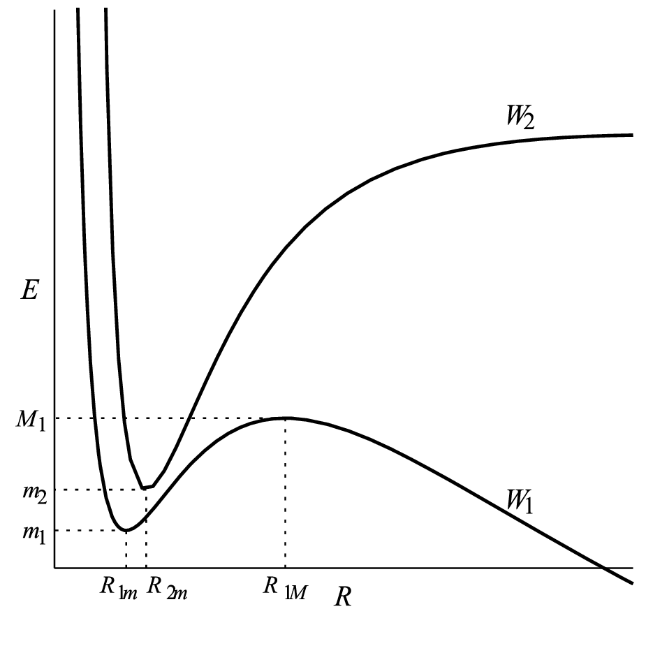
Hypothesis 3. The effective potential W1W_{1} has a single well shape, with local nondegenerate minimum value m1m_{1} at some point R1,mR_{1,m}, with a barrier with local nondegenerate maximum value M1M_{1} at some point R1,MR_{1,M}; beside, W1W_{1} does not admit other critical points in the domain W1−1​([m1,M1])W^{-1}_{1}\left([m_{1},M_{1}]\right). The effective potential W2W_{2} has a single well shape, with local minimum value m2m_{2} at some point R2,m>R⁡(1,m)R_{2,m}>R(1,m).

Remark 2.3.

In absence of the external field the local maximum value M1M_{1} disappears and we only have two local minimum values [Ci], in such a case ℰ1∞=ℰ2∞{\mathcal{E}}_{1}^{\infty}={\mathcal{E}}_{2}^{\infty} and we could treat the spectral problem for eigenvalues belonging to the interval [m1,M~1][m_{1},\widetilde{M}_{1}], for any M~1<ℰ1∞\widetilde{M}_{1}<{\mathcal{E}}_{1}^{\infty}. If the external field is small enough, but not zero, then we expect to observe a local maximum value such that m1<m2<M1m_{1}<m_{2}<M_{1} and R1,m<R2,m<R1,MR_{1,m}<R_{2,m}<R_{1,M} as in Fig. 1. For increasing external field, as considered by [MuSh], can happen to have m1<M1<m2m_{1}<M_{1}<m_{2}.

Refer to caption
Figure 1. Graph of the effective potentials W1​(R)W_{1}(R) and W2​(R)W_{2}(R) with single well shapes. The effective potential W1​(R)W_{1}(R) has a barrier and it does not admit other critical points in the domain W1−1​([m1,M1])W^{-1}_{1}\left([m_{1},M_{1}]\right); where m1m_{1} and M1M_{1} are the values of the local maximum and minimum point of W1W_{1}.

2.3. Spectrum of the reduced operator

In polar coordinates, Hamiltonian (1) takes the form,

H=−h2​[∂2∂R2+2R​∂∂R]−h2​1R2​Λ2+1R+He​(𝐑)\displaystyle H=-h^{2}\left[\frac{\partial^{2}}{\partial R^{2}}+\frac{2}{R}\frac{\partial}{\partial R}\right]-h^{2}\frac{1}{R^{2}}\Lambda^{2}+\frac{1}{R}+H_{e}(\mathbf{R}) (9)

where Λ2\Lambda^{2} is the Legendrian operator,

Λ2=1sin⁡θ​∂∂θ​sin⁡θ​∂∂θ+1sin2⁡θ​∂2∂φ2.\displaystyle\Lambda^{2}=\frac{1}{\sin\theta}\frac{\partial}{\partial\theta}{\sin\theta}\frac{\partial}{\partial\theta}+\frac{1}{\sin^{2}\theta}\frac{\partial^{2}}{\partial\varphi^{2}}.

The operator −h2​1R2​Λ2-h^{2}\frac{1}{R^{2}}\Lambda^{2} has eigenvalues h2​1R2​ℓ​(ℓ+1)h^{2}\frac{1}{R^{2}}\ell(\ell+1), ℓ∈{0,1,2,…}\ell\in\{0,1,2,\ldots\}. As a consequence, using Remark 2.2, a suitable choice of the rotation OO makes the operator HH take the form,

H=−h2​[∂2∂R2+2R​∂∂R]+h2​ℓ⁡(ℓ+1)R2+1R+He​(R)\displaystyle H=-h^{2}\left[\frac{\partial^{2}}{\partial R^{2}}+\frac{2}{R}\frac{\partial}{\partial R}\right]+h^{2}\frac{\ell(\ell+1)}{R^{2}}+\frac{1}{R}+H_{e}(R)

on L2​(ℝ+,R2​d​R,L2​(ℝ𝐫3))L^{2}(\mathbb{R}_{+},R^{2}dR;L^{2}(\mathbb{R}^{3}_{\mathbf{r}})). Finally, by taking ℓ=0\ell=0, that is, by considering the restriction of HH on K​e​r​(𝐋𝐑)Ker(\mathbf{L}_{\mathbf{R}}) (still denoted by HH), and by performing the change ψ⁡(R,𝐫)→R​ψ​(R,𝐫)\psi(R,\mathbf{r})\to R\psi(R,\mathbf{r}), the Hamiltonian HH takes the form,

H0=−h2​∂2∂R2+1R+He​(R)\displaystyle H_{0}=-h^{2}\frac{\partial^{2}}{\partial R^{2}}+\frac{1}{R}+H_{e}(R)

on L2​(ℝ+,d​R,L2​(ℝ𝐫3))L^{2}(\mathbb{R}_{+},dR;L^{2}(\mathbb{R}^{3}_{\mathbf{r}})) with Dirichlet boundary condition at R=0R=0.

Let PjP_{j}, j=1,2j=1,2, be the reduced operator formally defined by

Pj=−h2​d2d​R2+Wj​(R),Wj​(R)=1R+ℰj​(R),\displaystyle P_{j}=-h^{2}\frac{d^{2}}{dR^{2}}+W_{j}(R),\ \ W_{j}(R)=\frac{1}{R}+{\mathcal{E}}_{j}(R), (10)

on the Hilbert space L2​(ℝ+,d​R)L^{2}(\mathbb{R}_{+},dR) with Dirichlet boundary condition at R=0R=0.

Then, it follows that for hh small enough and for small external field, the discrete spectra of PjP_{j} in the interval [mj,ℰj∞)[m_{j},{\mathcal{E}}_{j}^{\infty}), j=1,2j=1,2, is not empty (see, e.g., [La] in the case without the external field), and we denote it by

Spd(Pj)={ekj,k≥1},j=1,2.\displaystyle{\mbox{Sp}}_{\text{d}}\left(P_{j}\right)=\left\{e_{k}^{j},\ k\geq 1\right\}\,,\ j=1,2\,.

In particular, in the case of non degenerate minima points m1m_{1} and m2m_{2}, combining results from [HeRo] and [HeSj1], we know that the gap ek+1j−ekje_{k+1}^{j}-e_{k}^{j} between two consecutive eigenvalues of PjP_{j} (j=1,2j=1,2) is of order hh as h→0+h\rightarrow 0_{+}, in the sense that cj​h≤ek+1j−ekj≤Cj​hc_{j}h\leq e_{k+1}^{j}-e_{k}^{j}\leq C_{j}h with cj,Cj>0c_{j},C_{j}>0 independent of hh and k=𝒪⁡(h−1)k=\mathcal{O}(h^{-1}).

2.4. Physical motivation

It is well known [Ca] that the dynamics of the three particle system called molecule-ion H2+H_{2}^{+}, referred to its center of mass, and under the effect of an external homogeneous field, is described by a Hamiltonian operator of the form,

H=−h2​Δ𝐑+Z2R+He\displaystyle H=-h^{2}\Delta_{\mathbf{R}}+\frac{Z^{2}}{R}+H_{e} (11)

where h≪1h\ll 1 is the effective semiclassical parameter given by the square root of the ratio between the light mass of the electron ee and the heavy mass (when compared with the electron mass) of the hydrogen nuclei. Moreover,

𝐑=x​𝐱^+y​𝐲^+z​𝐳^\displaystyle\mathbf{R}=x\hat{\mathbf{x}}+y\hat{\mathbf{y}}+z\hat{\mathbf{z}}

is the relative position of the two hydrogen nuclei of H2+H_{2}^{+}, and ZZ is the electron charge (hereafter, for the sake of definiteness we assume that the units are such that, Z=1Z=1). The electronic Hamiltonian (2) describes the relative motion of the electron ee referred to the fixed nuclei, and it actually depends on the nuclear distance RR, where VV is the potential of the external force.

Now we consider the isolated molecule. The asymptotic behavior for large RR of the functions Wj​(R)W_{j}(R) is dominated by the Van der Waals force given by,

Wj​(R)=−c4R4+O⁡(R−6),Wj′​(R)=4​c4R5+O⁡(R−7),W_{j}(R)=-\frac{c_{4}}{R^{4}}+O(R^{-6}),\,\,W_{j}^{\prime}(R)=4\frac{c_{4}}{R^{5}}+O(R^{-7}),

for a constant c4>0c_{4}>0 (see the constant E(4)E^{(4)} of [Ci]). The energy binding of the molecule, ℰ1∞−m1>0\mathcal{E}_{1}^{\infty}-m_{1}>0 is much smaller than the separation distance of the fundamental level of the atom ℰ3∞−ℰ1∞>0\mathcal{E}_{3}^{\infty}-\mathcal{E}_{1}^{\infty}>0.

Following [Hi, MuSh], we consider the case where the external field is a Stark-like field directed along the axes of the two nuclei, in agreement with Hyp. 1, with potential

V⁡(𝐑,𝐫)=−χ⁡(⟨𝐑R,𝐫⟩),R=|𝐑|,\displaystyle V(\mathbf{R},\mathbf{r})=-\chi\left(\left\langle\frac{\mathbf{R}}{R},\mathbf{r}\right\rangle\right)\,,\ R=|\mathbf{R}|\,, (12)

where χ\chi is a real-valued function bounded from below. In such a case, the Hamiltonian HH commutes with the angular momentum 𝐋𝐑+𝐋𝐫\mathbf{L}_{\mathbf{R}}+\mathbf{L}_{\mathbf{r}}. In fact, the effective potentials W1​(R)W_{1}(R) and W2​(R)W_{2}(R) show a shape as in Fig. 1 (see, e.g., [MuSh], and Fig. 2 of [Ca]).

The function χ\chi admits an analytic extension to a complex strip containing the real axis. More precisely, we assume,

χ⁡(x)=χd​(x)=ν​x1+(x/d)2=d​ν1+(d/x)2=d​ν​(1−d22​x2+3​d48​x4+O⁡(d6x6)),\chi(x)=\chi_{d}(x)=\nu\frac{x}{\sqrt{1+(x/d)^{2}}}=\frac{d\nu}{\sqrt{1+(d/x)^{2}}}=d\nu(1-\frac{d^{2}}{2x^{2}}+\frac{3d^{4}}{8x^{4}}+O(\frac{d^{6}}{x^{6}})),

for x2>d2,x^{2}>d^{2}, where d>0d>0 is a parameter much larger than the molecular size.

For

Δ​ℰ​(R)=ℰ2​(R)−ℰ1​(R),\Delta\mathcal{E}(R)=\mathcal{E}_{2}(R)-\mathcal{E}_{1}(R),

small enough for R2>>d2R^{2}>>d^{2}, we can approximate with a degenerate perturbation with effective Stark potential for the nucleons given by the matrix element of the potential on the two electronic states ψj,R=ψj,R​(r)\psi_{j,R}=\psi_{j,R}(r),

VS(R)=|<ψ1,R,V(𝐑,.)ψ2,R>|=Cχ(R)=δ(1−d22​R2+3​d48​R4+O(d6R6)),\displaystyle V_{S}(R)=|<\psi_{1,R},V(\mathbf{R},.)\psi_{2,R}>|=C\chi(R)=\delta(1-\frac{d^{2}}{2R^{2}}+\frac{3d^{4}}{8R^{4}}+O(\frac{d^{6}}{R^{6}})), (13)

where δ=C​d​ν>0\delta=Cd\nu>0. Thus, for large RR, the two nuclear potentials are bounded and behaves as in Fig. 1,

W1​(R)=ℰ1∞−δ⁡(1−d22​R2)−(c4+δ​3​d48)​1R4+O⁡(1/R6),W_{1}(R)=\mathcal{E}_{1}^{\infty}-\delta(1-\frac{d^{2}}{2R^{2}})-(c_{4}+\delta\frac{3d^{4}}{8})\frac{1}{R^{4}}+O(1/R^{6}),
W2​(R)=ℰ1∞+δ⁡(1−d22​R2)−(c4−δ​3​d48)​1R4+O⁡(1/R6).W_{2}(R)=\mathcal{E}_{1}^{\infty}+\delta(1-\frac{d^{2}}{2R^{2}})-(c_{4}-\delta\frac{3d^{4}}{8})\frac{1}{R^{4}}+O(1/R^{6}).

If we admit derivation of the asymptotic series, we have a maximum R1,MR_{1,M} of W1​(R)W_{1}(R) diverging as δ→0\delta\rightarrow 0,

R1,M2∼4​c4δ​d2+3​d22.R_{1,M}^{2}\sim\frac{4c_{4}}{\delta d^{2}}+\frac{3d^{2}}{2}.

3. Analytic distortion and regularization of the operator

3.1. Analytic distortion

Let s∈C∞​(ℝ)s\in C^{\infty}({\mathbb{R}}), 0≤s≤10\leq s\leq 1 with s⁡(x)=0s(x)=0 in an arbitrarily large compact set containing 0, and s⁡(x)=1s(x)=1 if |x||x| is large enough. For μ\mu real small enough, we set,

Iμ:ℝ3→ℝ3,Iμ​(𝐑)=𝐑⁡(1+μ​s​(R))\displaystyle I_{\mu}:{\mathbb{R}}^{3}\rightarrow{\mathbb{R}}^{3},\quad I_{\mu}(\mathbf{R})=\mathbf{R}(1+\mu s(R)) (14)
Jμ:ℝ6→ℝ3,Jμ​(𝐑,𝐫)=𝐫⁡[1+μ​s​(⟨𝐑R,𝐫⟩)],\displaystyle J_{\mu}:{\mathbb{R}}^{6}\rightarrow{\mathbb{R}}^{3},\quad J_{\mu}(\mathbf{R},\mathbf{r})=\mathbf{r}\left[1+\mu s\left(\left\langle\frac{\mathbf{R}}{R},\mathbf{r}\right\rangle\right)\right], (15)

and we define the analytic distortion on the test function φ\varphi, by the formula,

(𝒮μ​φ)​(𝐑,𝐫)=|J⁡(𝐑,𝐫)|1/2​φ​(Iμ​(𝐑),Jμ​(𝐑,𝐫)),\displaystyle\left(\mathcal{S}_{\mu}\varphi\right)(\mathbf{R},\mathbf{r})=|J(\mathbf{R},\mathbf{r})|^{1/2}\varphi(I_{\mu}(\mathbf{R}),J_{\mu}(\mathbf{R},\mathbf{r})), (16)

where we have set R=|𝐑|R=|\mathbf{R}|, and J⁡(𝐑,𝐫)J(\mathbf{R},\mathbf{r}) is the Jacobian of the transformation FμF_{\mu} given by,

Fμ:ℝ6→ℝ6,Fμ​(𝐑,𝐫)=(Iμ​(𝐑),Jμ​(𝐑,𝐫)).\displaystyle F_{\mu}:{\mathbb{R}}^{6}\rightarrow{\mathbb{R}}^{6},F_{\mu}(\mathbf{R},\mathbf{r})=(I_{\mu}(\mathbf{R}),J_{\mu}(\mathbf{R},\mathbf{r})). (17)

We also set

ϕμ:ℝ+→ℝ+,ϕμ​(R)=R⁡(1+μ​s​(R)).\displaystyle\phi_{\mu}:{\mathbb{R}}_{+}\rightarrow{\mathbb{R}}_{+},\phi_{\mu}(R)=R(1+\mu s(R)).

Then, the analytic distortion applied to the operator (1) defined on the Hilbert space 𝒦\mathcal{K} takes the form,

Hμ=𝒮μ​H​𝒮μ−1=−h2​𝒮μ​Δ𝐑​𝒮μ−1+1ϕμ​(R)+Hμ,e​(𝐑),\displaystyle H_{\mu}=\mathcal{S}_{\mu}H\mathcal{S}_{\mu}^{-1}=-h^{2}\mathcal{S}_{\mu}\Delta_{\mathbf{R}}\mathcal{S}_{\mu}^{-1}+\frac{1}{\phi_{\mu}(R)}+H_{\mu,e}(\mathbf{R})\,, (18)

with Hμ,e​(𝐑)H_{\mu,e}(\mathbf{R}) given by,

Hμ,e​(𝐑)=−𝒮μ​Δ𝐫​𝒮μ−1−1|Jμ​(𝐑,𝐫)−12​Iμ​(𝐑)|−1|Jμ​(𝐑,𝐫)+12​Iμ​(𝐑)|+Vμ,\displaystyle H_{\mu,e}(\mathbf{R})=-\mathcal{S}_{\mu}\Delta_{\mathbf{r}}\mathcal{S}_{\mu}^{-1}-\frac{1}{|J_{\mu}(\mathbf{R},\mathbf{r})-\frac{1}{2}I_{\mu}(\mathbf{R})|}-\frac{1}{|J_{\mu}(\mathbf{R},\mathbf{r})+\frac{1}{2}I_{\mu}(\mathbf{R})|}+V^{\mu},

where the distorted external potential is given by,

Vμ​(𝐑,𝐫)=V⁡[⟨𝐑R,𝐫⟩​(1+μ​s​(⟨𝐑R,𝐫⟩))].\displaystyle V_{\mu}(\mathbf{R},\mathbf{r})=V\left[\left\langle\frac{\mathbf{R}}{R},\mathbf{r}\right\rangle\left(1+\mu s\left(\left\langle\frac{\mathbf{R}}{R},\mathbf{r}\right\rangle\right)\right)\right].

Thus, Hμ,e​(𝐑)H_{\mu,e}(\mathbf{R}) can be extended to small enough complex values of μ\mu as an analytic family of type A.

Remark 3.1.

We also observe that, if OO is a rotation in ℝ3\mathbb{R}^{3}, then,

Iμ​(O​𝐑)=O​Iμ​(𝐑);Jμ​(O​𝐑,O​𝐫)=O​Jμ​(𝐑,𝐫).\displaystyle I_{\mu}(O\mathbf{R})=OI_{\mu}(\mathbf{R})\quad;\quad J_{\mu}(O\mathbf{R},O\mathbf{r})=OJ_{\mu}(\mathbf{R},\mathbf{r})\,.

As a consequence,

[𝒮μ,𝐋𝐑+𝐋𝐫]=0,\displaystyle[\mathcal{S}_{\mu},\mathbf{L}_{\mathbf{R}}+\mathbf{L}_{\mathbf{r}}]=0, (19)

and,

Hμ,e​(O​𝐑,O​𝐫,O−1​D𝐫)=Hμ,e​(𝐑,𝐫,D𝐫).\displaystyle H_{\mu,e}(O\mathbf{R},O\mathbf{r},O^{-1}D_{\mathbf{r}})=H_{\mu,e}(\mathbf{R},\mathbf{r},D_{\mathbf{r}}).

We denote by Hμ,0H_{\mu,0} the restriction of Hμ,e​(𝐑,𝐫,D𝐫)H_{\mu,e}(\mathbf{R},\mathbf{r},D_{\mathbf{r}}) to the invariant subspace K​e​r​(𝐋𝐑+𝐋𝐫)Ker(\mathbf{L}_{\mathbf{R}}+\mathbf{L}_{\mathbf{r}}).

3.2. Regularization of HμH_{\mu}

In this section, we want to regularize the operator HμH_{\mu} with respect to the 𝐑\mathbf{R}-variable. Having in mind the representation (9) of the Laplacian in polar coordinates, we denote

Ω⁡(1/M):={𝐑∈ℝ3:R>1M},Ω0​(1/M):={𝐑∈ℝ3:R<1M},\displaystyle\Omega(1/M):=\left\{\mathbf{R}\in{\mathbb{R}}^{3}\;:\;R>\frac{1}{M}\right\},\ \ \Omega_{0}(1/M):=\left\{\mathbf{R}\in{\mathbb{R}}^{3}\;:\;R<\frac{1}{M}\right\}\,,

and S2S^{2} is the unit sphere in ℝ𝐑3\mathbb{R}^{3}_{\mathbf{R}}, and

L0:=−Δ𝐫+C0\displaystyle L_{0}:=-\Delta_{\mathbf{r}}+C_{0}

with C0,M>0C_{0},M>0 large enough. We have the following preliminary technical lemma:

Lemma 3.2.

Under the previous assumptions, there exists a finite family of conical open sets (Ωℓ)ℓ=1m(\Omega_{\ell})_{\ell=1}^{m} in ℝ3{\mathbb{R}}^{3}, of the form Ωℓ=]1M,+∞[×ωℓ\Omega_{\ell}=]\frac{1}{M},+\infty[\times\omega_{\ell} with ωℓ\omega_{\ell} bounded open set of S2S^{2}, and a corresponding family of unitary operators 𝒰ℓ​(𝐑)\mathcal{U}_{\ell}(\mathbf{R}) (ℓ=1,⋯,m\ell=1,\cdots,m, 𝐑∈Ωℓ\mathbf{R}\in\Omega_{\ell}) on L2​(ℝ𝐫3)L^{2}(\mathbb{R}^{3}_{\mathbf{r}}), such that (denoting by UℓU_{\ell} the unitary operator on L2​(Ωℓ,L2​(ℝ𝐫3))≃L2​(Ωℓ)⊗L2​(ℝ𝐫3)L^{2}(\Omega_{\ell};L^{2}({\mathbb{R}}^{3}_{\mathbf{r}}))\simeq L^{2}(\Omega_{\ell})\otimes{L^{2}({\mathbb{R}}^{3}_{\mathbf{r}}}) induced by the action of 𝒰ℓ​(𝐑)\mathcal{U}_{\ell}(\mathbf{R}) on L2​(ℝ𝐫3)L^{2}({\mathbb{R}}^{3}_{\mathbf{r}})), one has,

  1. (1)

    Ω(1/M)=∪ℓ=1mΩℓ\Omega(1/M)=\mathop{\displaystyle\cup_{\ell=1}^{m}\Omega_{\ell}};

  2. (2)

    For all ℓ=1,⋯,m\ell=1,\cdots,m and 𝐑∈Ωℓ\mathbf{R}\in\Omega_{\ell}, 𝒰ℓ​(𝐑)\mathcal{U}_{\ell}(\mathbf{R}) leaves H2​(ℝ𝐫3)H^{2}({\mathbb{R}}^{3}_{\mathbf{r}}) invariant;

  3. (3)

    For all ℓ\ell, the operator 𝒰ℓ​(−h2​𝒮μ​Δ𝐑​𝒮μ−1)​𝒰ℓ−1\mathcal{U}_{\ell}(-h^{2}\mathcal{S}_{\mu}\Delta_{\mathbf{R}}\mathcal{S}_{\mu}^{-1})\mathcal{U}_{\ell}^{-1} is a semiclassical differential operator with operator-valued symbols, of the form,

    −h2​𝒮μ​Δ𝐑​𝒮μ−1+h​∑|β|=1ωβ,ℓ​(𝐑)​(h​D𝐑)β+h2​ω0,ℓ​(𝐑),D𝐑=−i​∇𝐑-h^{2}\mathcal{S}_{\mu}\Delta_{\mathbf{R}}\mathcal{S}_{\mu}^{-1}+h\sum_{|\beta|=1}\omega_{\beta,\ell}(\mathbf{R})(hD_{\mathbf{R}})^{\beta}+h^{2}\omega_{0,\ell}(\mathbf{R})\,,\ D_{\mathbf{R}}=-i\nabla_{\mathbf{R}} (20)

    where ωβ,ℓ​L0|β|2−1∈C∞​(Ωℓ;ℒ⁡(L2​(ℝ𝐫3))CLOSE\omega_{\beta,\ell}L_{0}^{\frac{|\beta|}{2}-1}\in C^{\infty}(\Omega_{\ell};{\mathcal{L}}(L^{2}({\mathbb{R}}^{3}_{\mathbf{r}})), and, for any γ∈ℕ3\gamma\in\mathbb{N}^{3}, the quantity ‖∂xγωβ,ℓ​(x)​L0|β|2−1‖ℒ⁡(L2​(ℝ𝐫3))\|\partial_{x}^{\gamma}\omega_{\beta,\ell}(x)L_{0}^{\frac{|\beta|}{2}-1}\|_{{\mathcal{L}}(L^{2}({\mathbb{R}}^{3}_{\mathbf{r}}))} is bounded uniformly with respect to hh small enough and locally uniformly with respect to x∈Ωℓx\in\Omega_{\ell};

  4. (4)

    For all ℓ\ell, the operators 𝒰ℓ​Hμ,e​𝒰ℓ−1\mathcal{U}_{\ell}H_{\mu,e}\mathcal{U}_{\ell}^{-1} are in C∞​(Ωℓ;ℒ⁡(H2​(ℝ𝐫3),L2​(ℝ𝐫3))CLOSEC^{\infty}(\Omega_{\ell};{\mathcal{L}}(H^{2}({\mathbb{R}}^{3}_{\mathbf{r}}),L^{2}({\mathbb{R}}^{3}_{\mathbf{r}})).

Proof.

At first, let us make a change of variables as in [MaMe], that localizes into a compact set the 𝐑\mathbf{R} - dependent singularities appearing into the interaction potential. Let χ∈C∞​(ℝ+)\chi\in C^{\infty}({\mathbb{R}}^{+}) satisfying 0≤χ≤1,χ′≤00\leq\chi\leq 1,\chi^{\prime}\leq 0, such that,

χ⁡(s)=1,if​  0≤s≤1,χ⁡(s)=0,if​s≥2\chi(s)=1,\;\;\;\;\mbox{if}\;\;0\leq s\leq 1,\quad\quad\chi(s)=0,\;\;\mbox{if}\;\;s\geq 2

For τ>1/2​M\tau>1/2M and τ>0\tau>0, we consider the function,

ρ⁡(τ,t)=tτ​χ​(tτ)+2​M​t​(1−χ⁡(tτ)).\rho(\tau,t)=\frac{t}{\tau}\chi\left(\frac{t}{\tau}\right)+2Mt\left(1-\chi\left(\frac{t}{\tau}\right)\right).

Then, it is easy to check that

∂ρ∂t>0on ]12​M,+∞[×ℝ+,\displaystyle\frac{\partial\rho}{\partial t}>0\;\;\mbox{on }\left]\frac{1}{2M},+\infty\right[\times{\mathbb{R}}_{+},
ρ​is surjective onto ​ℝ+,\displaystyle\rho\;\;\mbox{is surjective onto }{\mathbb{R}}_{+},
∂kρ∂τkis uniformly bounded on ]12​M,+∞[×ℝ+,∀k≥1.\displaystyle\frac{\partial^{k}\rho}{\partial\tau^{k}}\;\;\mbox{is uniformly bounded on }]\frac{1}{2M},+\infty[\times{\mathbb{R}}_{+},\forall k\geq 1.

Therefore we can define ατ\alpha_{\tau} as the inverse diffeomorphism on ℝ+{\mathbb{R}}_{+} of the function t→ρ⁡(τ,t)t\rightarrow\rho(\tau,t). in particular, by construction we have,

ατ​(t)=t2​M​if​t≥4​M​τ,ατ​(t)=τ​t​if​t≤1.\alpha_{\tau}(t)=\frac{t}{2M}\;\;\mbox{if}\;\;t\geq 4M\tau,\quad\alpha_{\tau}(t)=\tau t\;\;\mbox{if}\;\;t\leq 1.

Now, for 𝐑∈Ω⁡(1/M)\mathbf{R}\in\Omega(1/M), we define

θ(𝐑,.):ℝ3→ℝ3,θ(𝐑,𝐫)=αR/2(|𝐫|)𝐫|𝐫|.\theta(\mathbf{R},.):{\mathbb{R}}^{3}\rightarrow{\mathbb{R}}^{3},\quad\theta(\mathbf{R},\mathbf{r})=\alpha_{R/2}(|\mathbf{r}|)\frac{\mathbf{r}}{|\mathbf{r}|}.

Then, for any 𝐑∈Ω⁡(1/M)\mathbf{R}\in\Omega(1/M), the function θ(𝐑,.)\theta(\mathbf{R},.) is a diffeomorphism of ℝ3{\mathbb{R}}^{3}, it depends smoothly on 𝐑\mathbf{R}, and is such that ∂𝐑αθ⁡(𝐑,𝐫)\partial_{\mathbf{R}}^{\alpha}\theta(\mathbf{R},\mathbf{r}) is uniformly bounded on Ω⁡(1/2​M)×ℝ3\Omega(1/2M)\times{\mathbb{R}}^{3}, for any α∈ℕ3∖{0}\alpha\in{\mathbb{N}}^{3}\setminus\{0\} (see [MaMe], Lemma 3.1). Moreover

θ⁡(𝐑,𝐑R)=𝐑2,\displaystyle\theta\left(\mathbf{R},\frac{\mathbf{R}}{R}\right)=\frac{\mathbf{R}}{2},
θ⁡(𝐑,𝐫)=𝐫2​M​for ​|𝐫|≥2​M​R,\displaystyle\theta(\mathbf{R},\mathbf{r})=\frac{\mathbf{r}}{2M}\;\;\;\mbox{for }|\mathbf{r}|\geq 2MR,
θ⁡(𝐑,𝐫)=R2​𝐫​for ​|𝐫|≤1.\displaystyle\theta(\mathbf{R},\mathbf{r})=\frac{R}{2}\mathbf{r}\;\;\;\mbox{for }|\mathbf{r}|\leq 1.

For R>1MR>\frac{1}{M}, we consider the unitary transformation on L2​(ℝ𝐫3)L^{2}({\mathbb{R}}^{3}_{\mathbf{r}}), given by,

(U⁡(𝐑)​ϕ)​(𝐫)=ϕ⁡(θ⁡(𝐑,𝐫))​|∂𝐫θ⁡(𝐑,𝐫)|1/2.(U(\mathbf{R})\phi)(\mathbf{r})=\phi(\theta(\mathbf{R},\mathbf{r}))|\partial_{\mathbf{r}}\theta(\mathbf{R},\mathbf{r})|^{1/2}\,.

The advantage of performing this change of variables is that the 𝐑\mathbf{R}-depending singularities of the potential are now localized in some compact subset of ℝ𝐫3{\mathbb{R}}^{3}_{\mathbf{r}}. Now, following the arguments of [KMSW] and with the help of the previous change of variables, let us show that, by a patch and cut procedure, one can localize the singularities of the potential at some fixed (𝐑\mathbf{R}-independent) points.

For any fixed z0∈S2z_{0}\in S^{2} (the unit sphere in ℝ3{\mathbb{R}}^{3}), we choose a functions fz0∈C0∞​(ℝ3,ℝ)f_{z_{0}}\in C_{0}^{\infty}(\mathbb{R}^{3};\mathbb{R}), such that,

fz0​(z0)=1,fz0​(−z0)=0f_{z_{0}}(z_{0})=1,\quad\quad f_{z_{0}}(-z_{0})=0

and, for zz close enough to z0z_{0} and s∈ℝ3s\in\mathbb{R}^{3}, we define

Fz0​(z,s):=s+(z−z0)​(fz0​(s)−fz0​(−s))∈ℝ3.F_{z_{0}}(z,s):=s+(z-z_{0})(f_{z_{0}}(s)-f_{z_{0}}(-s))\in\mathbb{R}^{3}.\\

For zz in a smooth neighborhood ωz0\omega_{z_{0}} of z0z_{0}, the application s↦Fz0​(z,s)s\mapsto F_{z_{0}}(z,s) is a diffeomorphism of ℝ3\mathbb{R}^{3}, and we have,

Fz0​(z,z0)=z,Fz0​(z,−z0)=−z.F_{z_{0}}(z,z_{0})=z,\quad F_{z_{0}}(z,-z_{0})=-z.

Moreover, for any α∈ℝ3\alpha\in{\mathbb{R}}^{3}, there exists Cα>0C_{\alpha}>0 such that, for any z∈ωz0z\in\omega_{z_{0}}, for any s,s′∈ℝ3s,s^{\prime}\in{\mathbb{R}}^{3}

1C0​|s−s′|≤|Fz0​(z,s)−Fz0​(z,s′)|≤C0​|s−s′|\displaystyle\frac{1}{C_{0}}|s-s^{\prime}|\leq|F_{z_{0}}(z,s)-F_{z_{0}}(z,s^{\prime})|\leq C_{0}|s-s^{\prime}|
|∂xαFz0​(z,s)−∂xαFz0​(z,s′)|≤Cα​|s−s′|\displaystyle|\partial_{x}^{\alpha}F_{z_{0}}(z,s)-\partial_{x}^{\alpha}F_{z_{0}}(z,s^{\prime})|\leq C_{\alpha}|s-s^{\prime}|
|∂xαFz0​(z,s)|≤C0,|α|≥1\displaystyle|\partial_{x}^{\alpha}F_{z_{0}}(z,s)|\leq C_{0},\quad|\alpha|\geq 1

If (ωℓ)ℓ=1m:=(ωzℓ)ℓ=1m(\omega_{\ell})_{\ell=1}^{m}:=(\omega_{z_{\ell}})_{\ell=1}^{m} is a family of such open sets that covers S2S^{2}, we set Fℓ(z,.):=Fzℓ(z,.)F_{\ell}(z,.):=F_{z_{\ell}}(z,.), and we define,

Ωℓ:=]1M,+∞[×ωℓ.\Omega_{\ell}:=\left]\frac{1}{M},+\infty\right[\times\omega_{\ell}.

For 𝐑∈Ωℓ\mathbf{R}\in\Omega_{\ell}, we also set,

(U~ℓ​(𝐑)​ϕ)​(𝐫)=|det⁡(∂𝐫Fℓ)​(𝐑R,𝐫)|1/2​ϕ​(Fℓ​(𝐑R,𝐫)),(\widetilde{U}_{\ell}(\mathbf{R})\phi)(\mathbf{r})=\left|{\rm det}(\partial_{\mathbf{r}}F_{\ell})\left(\frac{\mathbf{R}}{R},\mathbf{r}\right)\right|^{1/2}\phi\left(F_{\ell}\left(\frac{\mathbf{R}}{R},\mathbf{r}\right)\right),

and,

𝒰ℓ​(𝐑):=U~ℓ​(𝐑)​U​(𝐑);\mathcal{U}_{\ell}(\mathbf{R}):=\widetilde{U}_{\ell}(\mathbf{R})U(\mathbf{R});
OPEN(𝒰ℓ​(𝐑)​ϕ)​(𝐫))=ϕ⁡(γℓ​(𝐑,𝐫))​|det⁡(∂𝐫γℓ)​(𝐑,𝐫)|,(\mathcal{U}_{\ell}(\mathbf{R})\phi)(\mathbf{r}))=\phi(\gamma_{\ell}(\mathbf{R},\mathbf{r}))|{\rm det}(\partial_{\mathbf{r}}\gamma_{\ell})(\mathbf{R},\mathbf{r})|,

where

γℓ​(𝐑,𝐫)=θ⁡(𝐑,Fℓ​(𝐑R,𝐫)).\gamma_{\ell}(\mathbf{R},\mathbf{r})=\theta\left(\mathbf{R},F_{\ell}\left(\frac{\mathbf{R}}{R},\mathbf{r}\right)\right).

Then, it is easy to check (see [MaMe]) that 𝒰ℓ\mathcal{U}_{\ell} satisfy (1), (2), (3), and (4). This completes the proof of the lemma. ∎

Now, let us consider the spectral projection Π0​(𝐑)\Pi_{0}(\mathbf{R}) associated to {ℰ1​(R),ℰ2​(R)}\{{\mathcal{E}}_{1}(R),{\mathcal{E}}_{2}(R)\} of He​(𝐑)H_{e}(\mathbf{R}), where ℰ1​(R)\mathcal{E}_{1}(R) and ℰ2​(R)\mathcal{E}_{2}(R) are the first two (simple) eigenvalues of He​(𝐑)H_{e}(\mathbf{R}). If one denote by γ⁡(R)\gamma(R) a continuous simple loop in ℂ\mathbb{C} enclosing {ℰ1​(R),ℰ2​(R)}\{{\mathcal{E}}_{1}(R),{\mathcal{E}}_{2}(R)\} and having the rest of Sp​(He​(𝐑)){\mbox{Sp}}\left(H_{e}(\mathbf{R})\right) in its exterior, one can write Π0​(𝐑)\Pi_{0}(\mathbf{R}) as,

Π0​(𝐑)=12​π​i​∫γ⁡(R)(He​(𝐑)−z)−1​𝑑z.\displaystyle\Pi_{0}(\mathbf{R})=\frac{1}{2\pi i}\int_{\gamma(R)}(H_{e}(\mathbf{R})-z)^{-1}\;dz.

Moreover, for μ\mu complex small enough, one can define the projector,

Πμ,0​(𝐑)=12​π​i​∫γ⁡(R)(Hμ,e​(𝐑)−z)−1​𝑑z\displaystyle\Pi_{\mu,0}(\mathbf{R})=\frac{1}{2\pi i}\int_{\gamma(R)}(H_{\mu,e}(\mathbf{R})-z)^{-1}\;dz

satisfying (Πμ,0)∗=Πμ¯,0(\Pi_{\mu,0})^{*}=\Pi_{\bar{\mu},0}. We have the following

Lemma 3.3.

There exist two functions,

w1μ​(𝐑,𝐫),w2μ​(𝐑,𝐫)∈C0​(ℝ𝐑3,H2​(ℝ𝐫3))\displaystyle w_{1}^{\mu}(\mathbf{R},\mathbf{r}),w_{2}^{\mu}(\mathbf{R},\mathbf{r})\in C^{0}({\mathbb{R}}_{\mathbf{R}}^{3};H^{2}({\mathbb{R}}^{3}_{\mathbf{r}}))

depending analytically on μ\mu, and real-valued for μ\mu real, such that,

  • i.

    ⟨wkμ​(𝐑,𝐫),wlμ¯​(𝐑,𝐫)⟩L2​(ℝ𝐫3)=δk,l,k,l=1,2\langle w_{k}^{\mu}(\mathbf{R},\mathbf{r}),w_{l}^{\bar{\mu}}(\mathbf{R},\mathbf{r})\rangle_{L^{2}({\mathbb{R}}^{3}_{\mathbf{r}})}=\delta_{k,l},\quad k,l=1,2;

  • ii.

    wjμ∈C∞​(Ω0​(2/M),H2​(ℝ𝐫3))w_{j}^{\mu}\in C^{\infty}(\Omega_{0}(2/M);H^{2}({\mathbb{R}}^{3}_{\mathbf{r}})), j=1,2j=1,2, and, for 𝐑∈Ω⁡(3/M)\mathbf{R}\in\Omega(3/M), w1μ​(𝐑,𝐫)w_{1}^{\mu}(\mathbf{R},\mathbf{r}) and w2μ​(𝐑,𝐫)w_{2}^{\mu}(\mathbf{R},\mathbf{r}) form a basis of Ran​Π0μ{\rm Ran}\Pi_{0}^{\mu};

  • iii.

    For 𝐑∈Ω⁡(3/M)\mathbf{R}\in\Omega(3/M), w1μ​(𝐑,𝐫)w_{1}^{\mu}(\mathbf{R},\mathbf{r}) and w2μ​(𝐑,𝐫)w_{2}^{\mu}(\mathbf{R},\mathbf{r}) are eigenfunctions of Hμ,e​(𝐑)H_{\mu,e}(\mathbf{R}) associated to ℰ1​(ϕμ​(R)){\mathcal{E}}_{1}(\phi_{\mu}(R)) and ℰ2​(ϕμ​(R)){\mathcal{E}}_{2}(\phi_{\mu}(R)) respectively;

  • iv.

    For all ℓ=1,…,m\ell=1,\dots,m, one has 𝒰ℓ​(𝐑)​wjμ​(𝐑,𝐫)∈Cb∞​(Ωℓ​(M),H2​(ℝ𝐫3))\mathcal{U}_{\ell}(\mathbf{R})w_{j}^{\mu}(\mathbf{R},\mathbf{r})\in C_{b}^{\infty}(\Omega_{\ell}(M),H^{2}({\mathbb{R}}^{3}_{\mathbf{r}})), j=1,2j=1,2.

  • v.

    w1μw_{1}^{\mu} and w2μw_{2}^{\mu} can be chosen in such a way that,

    (𝐋𝐑+𝐋𝐫)​w1μ=(𝐋𝐑+𝐋𝐫)​w2μ=0(\mathbf{L}_{\mathbf{R}}+\mathbf{L}_{\mathbf{r}})w_{1}^{\mu}=(\mathbf{L}_{\mathbf{R}}+\mathbf{L}_{\mathbf{r}})w_{2}^{\mu}=0.

Proof.

Taking into account that (see (6)),

limR↦+∞ℰ1​(R)≠limR↦+∞ℰ2​(R),\displaystyle\lim_{R\mapsto+\infty}{\mathcal{E}}_{1}(R)\not=\lim_{R\mapsto+\infty}{\mathcal{E}}_{2}(R),

the points (i)-(iv) follow from Lemma 3.1 of [MaSo] and from the arguments of Proposition 5.1 in [MaMe]. Moreover, since ℰ1​(R){\mathcal{E}}_{1}(R) and ℰ2​(R){\mathcal{E}}_{2}(R) are non degenerate, the last point (v) follows from [KMSW], Theorem 2.1, and from (19). ∎

Thanks to the previous lemma, we see that the family (Uℓ,Ωℓ)ℓ=0,m(U_{\ell},\Omega_{\ell})_{\ell=0,m} (with Ω0=Ω0​(2/M),𝒰0=𝕀\Omega_{0}=\Omega_{0}(2/M),\mathcal{U}_{0}=\mathbb{I} and Ωℓ,𝒰ℓ\Omega_{\ell},\mathcal{U}_{\ell} defined in Lemma 3.2 and Lemma 3.3), is a regular unitary covering of L2​(ℝ𝐑3,L2​(ℝ𝐫3))L^{2}({\mathbb{R}}^{3}_{\mathbf{R}};L^{2}({\mathbb{R}}^{3}_{\mathbf{r}})) in the sense of [MaSo], Definition 4.1.

We set,

Π~μ,0​(𝐑)=⟨⋅,w1μ​(𝐑)⟩L2​(ℝ𝐫3)​w1μ​(𝐑)+⟨⋅,w2μ​(𝐑)⟩L2​(ℝ𝐫3)​w2μ​(𝐑)\displaystyle\widetilde{\Pi}_{\mu,0}(\mathbf{R})=\langle\cdot,w_{1}^{\mu}(\mathbf{R})\rangle_{L^{2}(\mathbb{R}_{\mathbf{r}}^{3})}w_{1}^{\mu}(\mathbf{R})+\langle\cdot,w_{2}^{\mu}(\mathbf{R})\rangle_{L^{2}(\mathbb{R}_{\mathbf{r}}^{3})}w_{2}^{\mu}(\mathbf{R})

so that Π~μ,0​(R)\widetilde{\Pi}_{\mu,0}(R) coincides with Πμ,0​(R)\Pi_{\mu,0}(R) for 𝐑∈Ω⁡(3/M)\mathbf{R}\in\Omega(3/M), and verify,

𝒰ℓ​(𝐑)​Π~μ,0​(𝐑)​𝒰ℓ​(𝐑)−1∈C∞​(Ωℓ,ℒ⁡(L2​(ℝ𝐫3))),\displaystyle\mathcal{U}_{\ell}(\mathbf{R})\widetilde{\Pi}_{\mu,0}(\mathbf{R})\mathcal{U}_{\ell}(\mathbf{R})^{-1}\in C^{\infty}(\Omega_{\ell},{\mathcal{L}}(L^{2}(\mathbb{R}_{\mathbf{r}}^{3}))),

for all ℓ=0,…,m\ell=0,\dots,m. Also observe that, for any rotation OO,

TO​Π~μ,0​(𝐑)=Π~μ,0​(𝐑)​TOT_{O}\widetilde{\Pi}_{\mu,0}(\mathbf{R})=\widetilde{\Pi}_{\mu,0}(\mathbf{R})T_{O}

or, equivalently, [Πμ,0​(𝐑),𝐋𝐑+𝐋𝐫]=0[\Pi_{\mu,0}(\mathbf{R}),\mathbf{L}_{\mathbf{R}}+\mathbf{L}_{\mathbf{r}}]=0.

We also denote by Π~0​(𝐑)\widetilde{\Pi}_{0}(\mathbf{R}) the value of Π~μ,0​(𝐑)\widetilde{\Pi}_{\mu,0}(\mathbf{R}) for μ=0\mu=0.

Now, with the help of Π~μ,0​(𝐑)\widetilde{\Pi}_{\mu,0}(\mathbf{R}), we modify Hμ,e​(𝐑)H_{\mu,e}(\mathbf{R}) outside a neighborhood of Ω⁡(5/M)\Omega(5/M) as follows (see Proposition 3.2 in [MaSo]).

Proposition 3.4.

We choose a function ζ∈C∞​(ℝ+,[0,1])\zeta\in C^{\infty}(\mathbb{R}_{+};[0,1]), such that ζ=1\zeta=1 for R≥3/MR\geq 3/M and suppζ⊆]2/M,+∞[\mbox{\rm supp}\zeta\subseteq]2/M,+\infty[. Then, for all 𝐑∈ℝ3\mathbf{R}\in\mathbb{R}^{3}, and μ\mu complex small enough, there exists an operator H~μ,e​(𝐑)\widetilde{H}_{\mu,e}(\mathbf{R}) on L2​(ℝ𝐫3)L^{2}(\mathbb{R}_{\mathbf{r}}^{3}), with domain H2​(ℝ𝐫3)H^{2}(\mathbb{R}_{\mathbf{r}}^{3}), depending analytically on μ\mu, such that,

H~μ,e​(𝐑)=Hμ,e​(𝐑)if​𝐑∈Ω⁡(4/M);\displaystyle\widetilde{H}_{\mu,e}(\mathbf{R})=H_{\mu,e}(\mathbf{R})\quad\;\;\mbox{if}\,\,\mathbf{R}\in\Omega(4/M);
[H~μ,e​(𝐑),Π~μ,0​(𝐑)]=0for all ​𝐑∈ℝ3,\displaystyle[\widetilde{H}_{\mu,e}(\mathbf{R}),\widetilde{\Pi}_{\mu,0}(\mathbf{R})]=0\quad\;\;\mbox{for all }\mathbf{R}\in{\mathbb{R}}^{3},

and the application 𝐑↦𝒰ℓ​(𝐑)​H~μ,e​(𝐑)​𝒰ℓ​(𝐑)−1\mathbf{R}\mapsto\mathcal{U}_{\ell}(\mathbf{R})\widetilde{H}_{\mu,e}(\mathbf{R})\mathcal{U}_{\ell}(\mathbf{R})^{-1} is in C∞​(Ωℓ;ℒ⁡(H2​(ℝ𝐫3),L2​(ℝ𝐫3))𝐶𝐿𝑂𝑆𝐸C^{\infty}(\Omega_{\ell};{\mathcal{L}}(H^{2}(\mathbb{R}_{\mathbf{r}}^{3}),L^{2}(\mathbb{R}_{\mathbf{r}}^{3})) for all ℓ=0,…,m\ell=0,\dots,m. Moreover, H~μ,e​(𝐑)\widetilde{H}_{\mu,e}(\mathbf{R}) commutes with 𝐋𝐑+𝐋𝐫\mathbf{L}_{\mathbf{R}}+\mathbf{L}_{\mathbf{r}}, in the sense that, for any φ∈C0∞​(ℝ6)\varphi\in C_{0}^{\infty}(\mathbb{R}^{6}), one has,

(𝐋𝐑+𝐋𝐫)​H~μ,e​(𝐑)​φ=H~μ,e​(𝐑)​(𝐋𝐑+𝐋𝐫)​φ.(\mathbf{L}_{\mathbf{R}}+\mathbf{L}_{\mathbf{r}})\widetilde{H}_{\mu,e}(\mathbf{R})\varphi=\widetilde{H}_{\mu,e}(\mathbf{R})(\mathbf{L}_{\mathbf{R}}+\mathbf{L}_{\mathbf{r}})\varphi.

Hence, the spectrum of H~μ,e​(𝐑)\widetilde{H}_{\mu,e}(\mathbf{R}) actually depends only on R∈ℝ+R\in\mathbb{R}_{+}. Moreover, for μ\mu real, H~μ,e​(𝐑)\widetilde{H}_{\mu,e}(\mathbf{R}) is selfadjoint, uniformly semibounded from below, and the bottom of its spectrum consists in two eigenvalues,

ℰ~jμ(R)=ℰ~j(ϕμ(R)),j=1,2,\displaystyle\widetilde{\mathcal{E}}_{j}^{\mu}(R)=\widetilde{\mathcal{E}}_{j}(\phi_{\mu}(R))\,,\ j=1,2,

where

ℰ~j​(R)=ζ⁡(R)​ℰj​(R).\displaystyle\widetilde{\mathcal{E}}_{j}(R)=\zeta(R){\mathcal{E}}_{j}(R)\,.

Furthermore, H~μ,e​(𝐑)\widetilde{H}_{\mu,e}(\mathbf{R}) admits a global gap in its spectrum, in the sense that,

infR∈ℝ+dist​({ℰ~1μ​(R),ℰ~2μ​(R)},ℰ~3μ​(R))>0.\displaystyle\inf_{R\in\mathbb{R}_{+}}{\mbox{\rm dist}}(\{\widetilde{\mathcal{E}}_{1}^{\mu}(R),\widetilde{\mathcal{E}}_{2}^{\mu}(R)\},\widetilde{\mathcal{E}}_{3}^{\mu}(R))>0.

where we set

ℰ~3μ​(R)=Sp​(H~μ,e​(𝐑))\{ℰ~1μ​(R),ℰ~2μ​(R)}\displaystyle\widetilde{\mathcal{E}}_{3}^{\mu}(R)={\mbox{\rm Sp}}(\widetilde{H}_{\mu,e}(\mathbf{R}))\backslash\{\widetilde{\mathcal{E}}_{1}^{\mu}(R),\widetilde{\mathcal{E}}_{2}^{\mu}(R)\}
Proof.

The proof is similar to that of Proposition 3.2 in [MaSo], and we write it for μ=0\mu=0 only (the general case is obtained by just substituting Hμ,eH_{\mu,e} to HeH_{e} and Π~μ,0\widetilde{\Pi}_{\mu,0} to Π~0\widetilde{\Pi}_{0}). We set Π~0⟂​(𝐑)=1−Π~0​(𝐑)\widetilde{\Pi}_{0}^{\perp}(\mathbf{R})=1-\widetilde{\Pi}_{0}(\mathbf{R}) and

H~e​(𝐑)=ζ⁡(R)​He​(𝐑)+(1−ζ⁡(R))​Π~0⟂​(𝐑)​(−Δ𝐫+C0)​Π~0⟂​(𝐑).\displaystyle\widetilde{H}_{e}(\mathbf{R})=\zeta(R)H_{e}(\mathbf{R})+(1-\zeta(R))\widetilde{\Pi}_{0}^{\perp}(\mathbf{R})(-\Delta_{\mathbf{r}}+C_{0})\widetilde{\Pi}_{0}^{\perp}(\mathbf{R}).

with C0>0C_{0}>0 large enough and such that C0>ℰ¯3C_{0}>{\bar{\mathcal{E}}_{3}}, where

ℰ¯3:=infRℰ3​(R).\displaystyle{\bar{\mathcal{E}}_{3}}:=\inf_{R}{\mathcal{E}}_{3}(R)\,. (21)

Since Π~0​(𝐑)=Π0​(𝐑)\widetilde{\Pi}_{0}(\mathbf{R})=\Pi_{0}(\mathbf{R}) on Supp​ζ{\rm Supp}\hskip 1.0pt\zeta, we see that Π~0​(𝐑)\widetilde{\Pi}_{0}(\mathbf{R}) commutes with H~e​(𝐑)\widetilde{H}_{e}(\mathbf{R}), and it is also clear that H~e​(𝐑)\widetilde{H}_{e}(\mathbf{R}) is selfadjoint with domain H2​(ℝ3)H^{2}({\mathbb{R}}^{3}). Moreover,

Π~0​(𝐑)​He​(𝐑)​Π~0​(𝐑)=ζ⁡(𝐑)​Π0​(𝐑)​He​(𝐑)​Π0​(𝐑),\displaystyle\widetilde{\Pi}_{0}(\mathbf{R})H_{e}(\mathbf{R})\widetilde{\Pi}_{0}(\mathbf{R})=\zeta(\mathbf{R})\Pi_{0}(\mathbf{R})H_{e}(\mathbf{R})\Pi_{0}(\mathbf{R}),

and,

Π~0⟂​(𝐑)​H~e​(𝐑)​Π~0⟂​(𝐑)≥(ζ⁡(R)​ℰ3​(R)+(1−ζ⁡(R))​C0)​Π~0⟂​(𝐑)≥ℰ¯3​Π~0⟂​(𝐑).\widetilde{\Pi}_{0}^{\perp}(\mathbf{R})\widetilde{H}_{e}(\mathbf{R})\widetilde{\Pi}_{0}^{\perp}(\mathbf{R})\geq\left(\zeta(R){\mathcal{E}}_{3}(R)+(1-\zeta(R))C_{0}\right)\widetilde{\Pi}_{0}^{\perp}(\mathbf{R})\geq{\bar{\mathcal{E}}_{3}}\widetilde{\Pi}_{0}^{\perp}(\mathbf{R}). (22)

In particular, the bottom of the spectrum of H~e​(𝐑)\widetilde{H}_{e}(\mathbf{R}) consists in two eigenvalues ℰ~j​(R)=ζ⁡(R)​ℰj​(R)\widetilde{\mathcal{E}}_{j}(R)=\zeta(R){\mathcal{E}}_{j}(R) with associated eigenvectors Π~0​(𝐑)​ψj\widetilde{\Pi}_{0}(\mathbf{R})\psi_{j}, j=1,2j=1,2, where ℰj\mathcal{E}_{j} and ψj\psi_{j} are the first two eigenvalues and eigenvectors of (7). Furthermore, one has

infR>2/Mdist⁡(ℰ~3​(R),{ℰ~1​(R),ℰ~2​(R)})\displaystyle\inf_{R>2/M}{\rm dist}(\widetilde{\mathcal{E}}_{3}(R),\{\widetilde{\mathcal{E}}_{1}(R),\widetilde{\mathcal{E}}_{2}(R)\})
≥infR>2/M(ζ⁡(R)​( inf ​[ℰ3​(R)]−ℰ2​(R))+(1−ζ⁡(R))​C0)>0,\displaystyle\hskip 85.35826pt\geq\inf_{R>2/M}\left(\zeta(R)(\mbox{ inf }\left[{\mathcal{E}}_{3}(R)\right]-{\mathcal{E}}_{2}(R))+(1-\zeta(R))C_{0}\right)>0,

and

inf0<R≤2/Mdist⁡(ℰ~3​(R),{ℰ~1​(R),ℰ~2​(R)})≥C0.\displaystyle\inf_{0<R\leq 2/M}{\rm dist}(\widetilde{\mathcal{E}}_{3}(R),\{\widetilde{\mathcal{E}}_{1}(R),\widetilde{\mathcal{E}}_{2}(R)\})\geq C_{0}.

In particular, H~e​(𝐑)\widetilde{H}_{e}(\mathbf{R}) admits a fix global gap in its spectrum as stated in the proposition. Finally, we see that H~e​(𝐑)\widetilde{H}_{e}(\mathbf{R}) commutes with 𝐋𝐑+𝐋𝐫\mathbf{L}_{\mathbf{R}}+\mathbf{L}_{\mathbf{r}}, and 𝒰ℓ​H~e​(𝐑)​𝒰ℓ−1\mathcal{U}_{\ell}\widetilde{H}_{e}(\mathbf{R})\mathcal{U}_{\ell}^{-1} depends smoothly on 𝐑\mathbf{R} in Ωℓ\Omega_{\ell} for all ℓ=0,…,m\ell=0,\dots,m. ∎

3.3. Regularization of the operator

Definition 3.5 (Regularization of HμH_{\mu}).

Let 𝒮μ\mathcal{S}_{\mu} be the analytic distortion defined in (16) for μ\mu in some small complex neighborhood of zero, and let H~μ,e​(𝐑)\widetilde{H}_{\mu,e}(\mathbf{R}) and ζ⁡(R)\zeta(R) be defined as in Proposition 3.4. Then, we define the regularization of HμH_{\mu} as,

H~μ=−h2​𝒮μ​Δ𝐑​𝒮μ−1+H~μ,e​(𝐑)+ζ⁡(R)ϕμ​(R)+M3​(1−ζ⁡(R)).\displaystyle\widetilde{H}_{\mu}=-h^{2}\mathcal{S}_{\mu}\Delta_{\mathbf{R}}\mathcal{S}_{\mu}^{-1}+\widetilde{H}_{\mu,e}(\mathbf{R})+\frac{\zeta(R)}{\phi_{\mu}(R)}+\frac{M}{3}(1-\zeta(R)). (23)

Taking into account Definition 4.4 in [MaSo], we see that Lemma 3.2, Proposition 3.4 and (19) imply,

Lemma 3.6.

The operator H~μ\widetilde{H}_{\mu} is a twisted PDO (of degree 2) on L2​(ℝ𝐑3,L2​(ℝ𝐫3))L^{2}(\mathbb{R}_{\mathbf{R}}^{3},L^{2}(\mathbb{R}_{\mathbf{r}}^{3})) (in the sense of Definition 5.1 in [MaSo]), associated with the regular unitary covering (𝒰ℓ,Ωℓ)ℓ=0,…,m(\mathcal{U}_{\ell},\Omega_{\ell})_{\ell=0,\dots,m}. Moreover, it commutes with 𝐋𝐑+𝐋𝐫\mathbf{L}_{\mathbf{R}}+\mathbf{L}_{\mathbf{r}}.

Now, we define

Zμ+:L2​(ℝ6)→L2​(ℝ𝐑3)⊕L2​(ℝ𝐑3)\displaystyle Z_{\mu}^{+}:L^{2}(\mathbb{R}^{6})\rightarrow L^{2}(\mathbb{R}_{\mathbf{R}}^{3})\oplus L^{2}(\mathbb{R}_{\mathbf{R}}^{3})

by the formula,

(Zμ+​ψ)​(𝐑)=⟨ψ⁡(𝐑,⋅),w1μ¯​(𝐑,⋅)⟩L2​(ℝ𝐫3)⊕⟨ψ⁡(𝐑,⋅),w2μ¯​(𝐑,⋅)⟩L2​(ℝ𝐫3),\displaystyle\left(Z_{\mu}^{+}\psi\right)(\mathbf{R})=\langle\psi(\mathbf{R},\cdot),w_{1}^{\bar{\mu}}(\mathbf{R},\cdot)\rangle_{L^{2}(\mathbb{R}_{\mathbf{r}}^{3})}\oplus\langle\psi(\mathbf{R},\cdot),w_{2}^{\bar{\mu}}(\mathbf{R},\cdot)\rangle_{L^{2}({\mathbb{R}}_{\mathbf{r}}^{3})},

and,

Zμ−=(Zμ¯+)∗:L2​(ℝ𝐑3)⊕L2​(ℝ𝐑3)→L2​(ℝ6),\displaystyle Z_{\mu}^{-}=(Z_{\bar{\mu}}^{+})^{*}:L^{2}(\mathbb{R}_{\mathbf{R}}^{3})\oplus L^{2}(\mathbb{R}_{\mathbf{R}}^{3})\rightarrow L^{2}(\mathbb{R}^{6}),

by

(Zμ−​(u1⊕u2))​(𝐑,𝐫)=u1​(𝐑)​w1μ​(𝐑,𝐫)+u2​(𝐑)​w2μ​(𝐑,𝐫).\displaystyle\left(Z_{\mu}^{-}(u_{1}\oplus u_{2})\right)(\mathbf{R},\mathbf{r})=u_{1}(\mathbf{R})w_{1}^{\mu}(\mathbf{R},\mathbf{r})+u_{2}(\mathbf{R})w_{2}^{\mu}(\mathbf{R},\mathbf{r}).

Following [MaMe], we consider the Grushin problem,

𝒢~μ​(z)=(H~μ−zZμ−Zμ+0),\displaystyle\widetilde{\mathcal{G}}_{\mu}(z)=\left(\begin{array}[]{cc}\widetilde{H}_{\mu}-z&Z_{\mu}^{-}\\ Z_{\mu}^{+}&0\end{array}\right),

that sends H2​(ℝ6)⊕(L2​(ℝ3)⊕L2​(ℝ3))H^{2}(\mathbb{R}^{6})\oplus\left(L^{2}(\mathbb{R}^{3})\oplus L^{2}(\mathbb{R}^{3})\right) into L2​(ℝ6)⊕(H2​(ℝ3)⊕H2​(ℝ3))L^{2}(\mathbb{R}^{6})\oplus\left(H^{2}(\mathbb{R}^{3})\oplus H^{2}(\mathbb{R}^{3})\right).

Thanks to Lemma 3.3 and Lemma 3.6, we see that 𝒢~μ​(z)\widetilde{\mathcal{G}}_{\mu}(z) is a twisted PDO (of degree 2) on L2​(ℝ𝐑3,L2​(ℝ𝐫3)⊕ℂ⊕ℂ)L^{2}\left(\mathbb{R}^{3}_{\mathbf{R}};L^{2}(\mathbb{R}^{3}_{\mathbf{r}})\oplus\mathbb{C}\oplus\mathbb{C}\right), associated with the regular unitary covering (𝒱ℓ,Ωℓ)ℓ=0,…,m({\mathcal{V}}_{\ell},\Omega_{\ell})_{\ell=0,\dots,m}, where we have set

𝒱ℓ:=(𝒰ℓ0012).{\mathcal{V}}_{\ell}:=\left(\begin{array}[]{cc}\mathcal{U}_{\ell}&0\\ 0&1_{2}\end{array}\right).

We also have,

Lemma 3.7.

For all μ∈ℂ\mu\in\mathbb{C} small enough and z∈ℂz\in\mathbb{C}, the operator 𝒢~μ​(z)\widetilde{\mathcal{G}}_{\mu}(z) commutes with ℒ:=(L𝐑+L𝐫00L𝐑){\mathcal{L}}:=\left(\begin{array}[]{ccc}L_{\mathbf{R}}+L_{\mathbf{r}}&0\\ 0&L_{\mathbf{R}}\end{array}\right).

Proof.

By Lemma 3.6, we only need to study the commutation rules between Zμ±Z_{\mu}^{\pm} and the operators L𝐑L_{\mathbf{R}} and L𝐫L_{\mathbf{r}}. But, using Lemma 3.3, v., plus the fact that the formal adjoint of L𝐫L_{\mathbf{r}} is −L𝐫-L_{\mathbf{r}}, we immediately obtain,

(L𝐑+L𝐫)​Zμ−=Zμ−​L𝐑;L𝐑​Zμ+=Zμ+​(L𝐑+L𝐫),(L_{\mathbf{R}}+L_{\mathbf{r}})Z_{\mu}^{-}=Z_{\mu}^{-}L_{\mathbf{R}}\quad;\quad L_{\mathbf{R}}Z_{\mu}^{+}=Z_{\mu}^{+}(L_{\mathbf{R}}+L_{\mathbf{r}}),

and the result follows. ∎

Moreover, we see as in [MaMe], Section 5, that, for z∈ℂz\in\mathbb{C} with Re​z<infRℰ~3​(R){\rm Re}z<\inf_{R}\widetilde{\mathcal{E}}_{3}(R) and Im​z{\rm Im}z sufficiently small, the operator 𝒢~μ​(z)\widetilde{\mathcal{G}}_{\mu}(z) is invertible, and its inverse 𝒢~μ​(z)−1\widetilde{\mathcal{G}}_{\mu}(z)^{-1} is such that the operators,

(100⟨−Δ𝐑⟩−1)​𝒢~μ​(z)−1,𝒢~μ​(z)−1​(100⟨−Δ𝐑⟩−1)\left(\begin{array}[]{cc}1&0\\ 0&\langle-\Delta_{\mathbf{R}}\rangle^{-1}\end{array}\right)\widetilde{\mathcal{G}}_{\mu}(z)^{-1},\quad\widetilde{\mathcal{G}}_{\mu}(z)^{-1}\left(\begin{array}[]{cc}1&0\\ 0&\langle-\Delta_{\mathbf{R}}\rangle^{-1}\end{array}\right)

are twisted (bounded) hh-admissible operators associated with the regular unitary covering (𝒱ℓ,Ωℓ)ℓ=0,…,m({\mathcal{V}}_{\ell},\Omega_{\ell})_{\ell=0,\dots,m}. As a consequence, 𝒢~μ​(z)−1\widetilde{\mathcal{G}}_{\mu}(z)^{-1} can be written as,

𝒢~μ​(z)−1=(Eμ​(z)Eμ+​(z)Eμ−​(z)z−P~μ​(z)),\widetilde{\mathcal{G}}_{\mu}(z)^{-1}=\left(\begin{array}[]{cc}E_{\mu}(z)&E_{\mu}^{+}(z)\\ E_{\mu}^{-}(z)&z-\widetilde{P}_{\mu}(z)\end{array}\right),

where P~μ​(z)\widetilde{P}_{\mu}(z) is an unbounded hh-admissible operator on L2​(ℝ𝐑3)⊕L2​(ℝ𝐑3)L^{2}(\mathbb{R}_{\mathbf{R}}^{3})\oplus L^{2}(\mathbb{R}_{\mathbf{R}}^{3}) with domain H2​(ℝ𝐑3)⊕H2​(ℝ𝐑3)H^{2}(\mathbb{R}_{\mathbf{R}}^{3})\oplus H^{2}(\mathbb{R}_{\mathbf{R}}^{3}), and Eμ​(z)E_{\mu}(z), Eμ±​(z)E_{\mu}^{\pm}(z) are (bounded) twisted hh-admissible operators (all depending in a holomorphic way on zz).

More precisely, it results from [MaMe], formula (2.11), that the operator P~μ​(z)\widetilde{P}_{\mu}(z) is given by the formula,

P~μ​(z)=Zμ+​H~μ​Zμ−−Zμ+​[h2​𝒮μ​Δ𝐑​𝒮μ−1,Π~μ,0]​(H~μ′−z)−1​[Π~μ,0,h2​𝒮μ​Δ𝐑​𝒮μ−1]​Zμ−,\widetilde{P}_{\mu}(z)=Z_{\mu}^{+}\widetilde{H}_{\mu}Z_{\mu}^{-}-Z_{\mu}^{+}[h^{2}\mathcal{S}_{\mu}\Delta_{\mathbf{R}}\mathcal{S}_{\mu}^{-1},\widetilde{\Pi}_{\mu,0}](\widetilde{H}_{\mu}^{\prime}-z)^{-1}[\widetilde{\Pi}_{\mu,0},h^{2}\mathcal{S}_{\mu}\Delta_{\mathbf{R}}\mathcal{S}_{\mu}^{-1}]Z_{\mu}^{-}, (25)

where Π~μ,0\widetilde{\Pi}_{\mu,0} stands for the projection on L2​(ℝ6)L^{2}({\mathbb{R}}^{6}) induced by the action of Π~μ,0​(𝐑)\widetilde{\Pi}_{\mu,0}(\mathbf{R}) on L2​(ℝ𝐫3)L^{2}(\mathbb{R}_{\mathbf{r}}^{3}), and H~μ′\widetilde{H}_{\mu}^{\prime} is the restriction of (1−Π~μ,0)​H~μ​(1−Π~μ,0)(1-\widetilde{\Pi}_{\mu,0})\widetilde{H}_{\mu}(1-\widetilde{\Pi}_{\mu,0}) to the range of 1−Π~μ,01-\widetilde{\Pi}_{\mu,0}. In particular, H~μ′−z\widetilde{H}_{\mu}^{\prime}-z is invertible in virtue of (22), and Π~μ,0\widetilde{\Pi}_{\mu,0} is a twisted hh-admissible operator on L2​(ℝ𝐑3,L2​(ℝ𝐫3))L^{2}(\mathbb{R}_{\mathbf{R}}^{3},L^{2}(\mathbb{R}_{\mathbf{r}}^{3})) (in the sense of Definition 4.4 in [MaSo]), associated with the regular unitary covering (𝒰ℓ,Ωℓ)ℓ=0,…,m(\mathcal{U}_{\ell},\Omega_{\ell})_{\ell=0,\dots,m}.

By Lemma 3.7, we also know that P~μ​(z)\widetilde{P}_{\mu}(z) commutes with L𝐑L_{\mathbf{R}}, and thus, gathering all the previous information on P~μ​(z)\widetilde{P}_{\mu}(z), we finally obtain that it can be written as,

P~μ​(z)=−h2​𝒮μ​Δ𝐑​𝒮μ−1+ℳμ​(R)+h​𝒜μ​(𝐑,h​D𝐑)+h2​ℬμ​(𝐑,h​D𝐑,z,h)\displaystyle\widetilde{P}_{\mu}(z)=-h^{2}\mathcal{S}_{\mu}\Delta_{\mathbf{R}}\mathcal{S}_{\mu}^{-1}+{\mathcal{M}}_{\mu}(R)+h{\mathcal{A}}_{\mu}(\mathbf{R},h{\rm D}_{\mathbf{R}})+h^{2}{\mathcal{B}}_{\mu}(\mathbf{R},h{\rm D}_{\mathbf{R}};z,h) (26)

where, for any R>3MR>\frac{3}{M}, ℳμ{\mathcal{M}}_{\mu} is given by,

ℳμ​(R)=(W1​(ϕμ​(R))00W2​(ϕμ​(R))),Wj​(R)=ℰj​(R)+1R,\displaystyle{\mathcal{M}}_{\mu}(R)=\left(\begin{array}[]{cc}W_{1}(\phi_{\mu}(R))&0\\ 0&W_{2}(\phi_{\mu}(R))\end{array}\right)\,,W_{j}(R)={\mathcal{E}}_{j}(R)+\frac{1}{R}\,,

and, for R≤3MR\leq\frac{3}{M} and μ\mu sufficiently small, it satisfies,

Reℳμ​(R)≥M4+infRℰ1​(R).\displaystyle\mathop{\rm Re}\nolimits{\mathcal{M}}_{\mu}(R)\geq\frac{M}{4}+\inf_{R}{\mathcal{E}}_{1}(R). (30)

Here, MM is the same as in Proposition 3.4 and Definition 3.5, and it can be chosen arbitrarily large.

Moreover 𝒜μ​(𝐑,h​D𝐑){\mathcal{A}}_{\mu}(\mathbf{R},h{\rm D}_{\mathbf{R}}) is of the form,

𝒜μ=(0aμ​(𝐑)⋅h​D𝐑h​D𝐑⋅aμ¯​(𝐑)0),\displaystyle{\mathcal{A}}_{\mu}=\left(\begin{array}[]{cc}0&a_{\mu}(\mathbf{R})\cdot h{\rm D}_{\mathbf{R}}\\ h{\rm D}_{\mathbf{R}}\cdot\overline{a_{\mu}}(\mathbf{R})&0\end{array}\right),

for some smooth bounded (together with its derivatives) function aμ​(𝐑)a_{\mu}(\mathbf{R}) independent of zz. Finally, ℬμ​(𝐑,h​D𝐑,z,h){\mathcal{B}}_{\mu}(\mathbf{R},h{\rm D}_{\mathbf{R}};z,h) is an hh-admissible pseudodifferential operator depending analytically on zz, with Weyl symbol bμ​(𝐑,𝐑∗,z,h)b_{\mu}(\mathbf{R},\mathbf{R}^{*};z,h) holomorphic with respect to R∗R^{*} in a complex strip of the form {|ℑR∗|<δ}\{|\Im R^{*}|<\delta\} (with δ>0\delta>0 independent of zz and μ\mu), such that, for any multi-index α\alpha,

∂αbμ​(𝐑,𝐑∗,z,h)=𝒪⁡(1)\displaystyle\partial^{\alpha}b_{\mu}(\mathbf{R},\mathbf{R}^{*};z,h)=\mathcal{O}(1) (34)

uniformly with respect to (𝐑,𝐑∗)∈ℝ3×ℝ3(\mathbf{R},\mathbf{R}^{*})\in\mathbb{R}^{3}\times\mathbb{R}^{3}, h>0h>0 small enough, and zz close enough to some fix λ0∈ℂ\lambda_{0}\in\mathbb{C} such that Re​λ0<infRℰ~3​(R){\rm Re}\lambda_{0}<\inf_{R}\widetilde{\mathcal{E}}_{3}(R) and Im​λ0{\rm Im}\lambda_{0} sufficiently small.

Finally, the operators 𝒜μ{\mathcal{A}}_{\mu} and ℬμ​(𝐑,h​D𝐑,z,h){\mathcal{B}}_{\mu}(\mathbf{R},h{\rm D}_{\mathbf{R}};z,h) commute with L𝐑L_{\mathbf{R}}, and one has the Feshbach identities,

(H~μ−z)−1=Eμ​(z)+Eμ+​(z)​(P~μ​(z)−z)−1​Eμ−​(z),\displaystyle(\widetilde{H}_{\mu}-z)^{-1}=E_{\mu}(z)+E_{\mu}^{+}(z)(\widetilde{P}_{\mu}(z)-z)^{-1}E_{\mu}^{-}(z), (35)
(P~μ​(z)−z)−1=Zμ+​(H~μ−z)−1​Zμ−.\displaystyle(\widetilde{P}_{\mu}(z)-z)^{-1}=Z_{\mu}^{+}(\widetilde{H}_{\mu}-z)^{-1}Z_{\mu}^{-}.

Summing up, we have proved,

Theorem 3.8.

Let ℰ~3​(R)\widetilde{\mathcal{E}}_{3}(R) be defined as in Proposition 3.4 and let λ0∈ℂ\lambda_{0}\in\mathbb{C} with Re⁡(λ0)<infRℰ~3​(R){\rm Re}(\lambda_{0})<\inf_{R}\widetilde{\mathcal{E}}_{3}(R) and Im⁡(λ0){\rm Im}(\lambda_{0}) sufficiently small. Under the previous assumptions, there exists a complex neighborhood Dλ0D_{\lambda_{0}} of λ0\lambda_{0} such that, for any z∈Dλ0z\in D_{\lambda_{0}}, one has the equivalence,

z∈Sp⁡(H~μ)⟺z∈Sp⁡(P~μ​(z)),\displaystyle z\in{\rm Sp}(\widetilde{H}_{\mu})\Longleftrightarrow z\in{\rm Sp}(\widetilde{P}_{\mu}(z)),

where P~μ​(z)\widetilde{P}_{\mu}(z)is as in (26) with (3.3)-(34).

Now, taking advantage of Lemma 3.7, we can consider the restriction of the Grushin problem 𝒢~μ​(z)\widetilde{\mathcal{G}}_{\mu}(z) on K​e​r​(𝐋𝐑+𝐋𝐫)⊕K​e​r​(𝐋𝐑)⊕K​e​r​(𝐋𝐑)Ker(\mathbf{L}_{\mathbf{R}}+\mathbf{L}_{\mathbf{r}})\oplus Ker(\mathbf{L}_{\mathbf{R}})\oplus Ker(\mathbf{L}_{\mathbf{R}}), and we also immediately obtain,

Corollary 3.9.

Denote by H~μ0\widetilde{H}_{\mu}^{0} the restriction of H~μ\widetilde{H}_{\mu} on the invariant subspace K​e​r​(𝐋𝐑+𝐋𝐫)Ker(\mathbf{L}_{\mathbf{R}}+\mathbf{L}_{\mathbf{r}}), and by P~μ0​(z)\widetilde{P}_{\mu}^{0}(z) the restriction of P~μ​(z)\widetilde{P}_{\mu}(z) on the invariant subspace K​e​r​(𝐋𝐑)Ker(\mathbf{L}_{\mathbf{R}}). Then, for any λ0∈ℂ\lambda_{0}\in\mathbb{C} with Re⁡(λ0)<infRℰ~3​(R){\rm Re}(\lambda_{0})<\inf_{R}\widetilde{\mathcal{E}}_{3}(R) and Im⁡(λ0){\rm Im}(\lambda_{0}) sufficiently small, there exists a complex neighborhood Dλ0D_{\lambda_{0}} of λ0\lambda_{0} such that, for any z∈Dλ0z\in D_{\lambda_{0}}, one has the equivalence,

z∈Sp⁡(H~μ0)⟺z∈Sp⁡(P~μ0​(z)).\displaystyle z\in{\rm Sp}(\widetilde{H}_{\mu}^{0})\Longleftrightarrow z\in{\rm Sp}(\widetilde{P}_{\mu}^{0}(z)).

In the sequel, we also denote by Hμ0H_{\mu}^{0} the restriction of HμH_{\mu} on the invariant subspace K​e​r​(𝐋𝐑+𝐋𝐫)Ker(\mathbf{L}_{\mathbf{R}}+\mathbf{L}_{\mathbf{r}}).

4. Reduced problem

Let us introduce the following shortcut notation,

D=h​DR,DR=−i​dd​R.\displaystyle{\rm D}=h{\rm D}_{R}\,,\ {\rm D}_{R}=-i\frac{d}{dR}.

For all R>0R>0, we define,

Wj,μ​(R):=ζ⁡(R)​Wj​(ϕμ​(R))+M3​(1−ζ⁡(R)),W_{j,\mu}(R):=\zeta(R)W_{j}(\phi_{\mu}(R))+\frac{M}{3}(1-\zeta(R)),

where ζ\zeta is as in Proposition 3.4, and MM is taken large enough. In particular, Wj,μW_{j,\mu} is bounded and depends analytically on μ\mu.

Then, we set,

ℳμ0​(R):=(Wμ,1​(R)00Wμ,2​(R)),{\mathcal{M}}_{\mu}^{0}(R):=\left(\begin{array}[]{cc}W_{\mu,1}(R)&0\\ 0&W_{\mu,2}(R)\end{array}\right),

and we denote by 𝒜μ0​(R,h​DR){\mathcal{A}}_{\mu}^{0}(R,h{\rm D}_{R}) the restriction of the differential operator (actually, vector-field) 𝒜μ​(𝐑,h​D𝐑){\mathcal{A}}_{\mu}(\mathbf{R},h{\rm D}_{\mathbf{R}}) on the space K​e​r​(𝐋𝐑)Ker(\mathbf{L}_{\mathbf{R}}). In particular, since [𝒜μ,𝐋𝐑]=0[{\mathcal{A}}_{\mu},\mathbf{L}_{\mathbf{R}}]=0 then 𝒜μ0{\mathcal{A}}_{\mu}^{0} can be represented as a differential operator in the variable R=|𝐑|R=|\mathbf{R}|, and it can be written as,

𝒜μ0=𝒜μ0​(R,h​DR)=(0aμ0​(R)​h​DRh​DR⋅aμ0¯​(R)0),{\mathcal{A}}_{\mu}^{0}={\mathcal{A}}_{\mu}^{0}(R,h{\rm D}_{R})=\left(\begin{array}[]{cc}0&a_{\mu}^{0}(R)h{\rm D}_{R}\\ h{\rm D}_{R}\cdot\overline{a_{\mu}^{0}}(R)&0\end{array}\right),

where the function aμ0a_{\mu}^{0} is smooth and bounded together with all its derivatives on (0,+∞)(0,+\infty).

In this section, we look for the solutions to the eigenvalue equation,

Pμ♯​φ=λ​φ,λ∈ℂ,φ=(φ1φ2),\displaystyle P^{\sharp}_{\mu}\varphi=\lambda\varphi,\quad\lambda\in\mathbb{C},\,\,\varphi=\left(\begin{array}[]{c}\varphi_{1}\\ \varphi_{2}\end{array}\right),

where Pμ♯P^{\sharp}_{\mu} is the differential operator formally defined as,

Pμ♯=h2​𝒮μ​DR2​𝒮μ−1+ℳμ0​(R)+h​𝒜μ0​(R,h​DR)\displaystyle P^{\sharp}_{\mu}=h^{2}\mathcal{S}_{\mu}{\rm D}_{R}^{2}\mathcal{S}_{\mu}^{-1}+{\mathcal{M}}_{\mu}^{0}(R)+h{\mathcal{A}}_{\mu}^{0}(R,h{\rm D}_{R}) (39)

acting on the Hilbert space,

ℋ♯=L2([0,+∞),dR)⊕L2([0,+∞),dR),\displaystyle\mathcal{H}^{\sharp}=L^{2}\left([0,+\infty),dR\right)\oplus L^{2}\left([0,+\infty),dR\right), (40)

with zero Dirichlet boundary condition at R=0R=0, and where now, with abuse of notation, we denote,

(𝒮μ​φ)​(R)=|I′​(R)|1/2​φ​[I⁡(R)],I⁡(R)=R⁡[1+μ​s​(R)].\displaystyle\left(\mathcal{S}_{\mu}\varphi\right)(R)=|I^{\prime}(R)|^{1/2}\varphi[I(R)]\,,\ I(R)=R\left[1+\mu s(R)\right]\,. (41)

If we set,

Pj,μ=h2​𝒮μ​DR2​𝒮μ−1+Wj,μ​(R),\displaystyle P_{j,\mu}=h^{2}\mathcal{S}_{\mu}{\rm D}_{R}^{2}\mathcal{S}_{\mu}^{-1}+W_{j,\mu}(R)\,,

then equation (4) turns into

(P1,μ−λ)​φ1\displaystyle(P_{1,\mu}-\lambda)\,\varphi_{1} =−h​Aμ0​φ2;\displaystyle=-hA_{\mu}^{0}\varphi_{2}; (42)
(P2,μ−λ)​φ2\displaystyle(P_{2,\mu}-\lambda)\,\varphi_{2} =−h​Aμ0∗​φ1,\displaystyle=-h{A_{\mu}^{0}}^{*}\varphi_{1}, (43)

where

Aμ0=h​aμ0​(R)​DR.\displaystyle A_{\mu}^{0}=ha_{\mu}^{0}(R){\rm D}_{R}\,.

Let us also observe that, by the Weyl theorem, the essential spectrum of Pμ♯P_{\mu}^{\sharp} is given by,

Spe​s​s(Pμ♯)=ℰ1∞+(1+μ)−2[0,+∞).{\rm Sp}_{ess}(P^{\sharp}_{\mu})={\mathcal{E}}_{1}^{\infty}+(1+\mu)^{-2}[0,+\infty).

As before, mjm_{j} is the local minima of WjW_{j} and M1M^{1} is the local maximum of W1W^{1}, as defined in Remark 2.3. Now, for the sake of definiteness, we consider the case where

ℰ1∞<m1<m2<M1\displaystyle{\mathcal{E}}^{\infty}_{1}<m_{1}<m_{2}<M_{1} (44)

In the case where ℰ1∞<m1<M1<m2{\mathcal{E}}^{\infty}_{1}<m_{1}<M_{1}<m_{2} then we can apply the same argument to the interval [m1,M1][m_{1},M_{1}].

Remark 4.1.

By construction, we have Sp⁡(Hμ,e​(𝐑))=Sp⁡(He​(Iμ​(𝐑))𝐶𝐿𝑂𝑆𝐸{\rm Sp}(H_{\mu,e}(\mathbf{R}))={\rm Sp}(H_{e}(I_{\mu}(\mathbf{R})). Therefore, if the function s⁡(x)s(x) used in the distortion vanishes in a sufficiently compact set (and since Wj,μW_{j,\mu} and WjW_{j} coincide on this set), a continuity argument shows that, for μ∈ℂ\mu\in\mathbb{C} small enough, the critical points of ReWj,μ\mathop{\rm Re}\nolimits W_{j,\mu} and WjW_{j} coincide and remain non-degenerate.

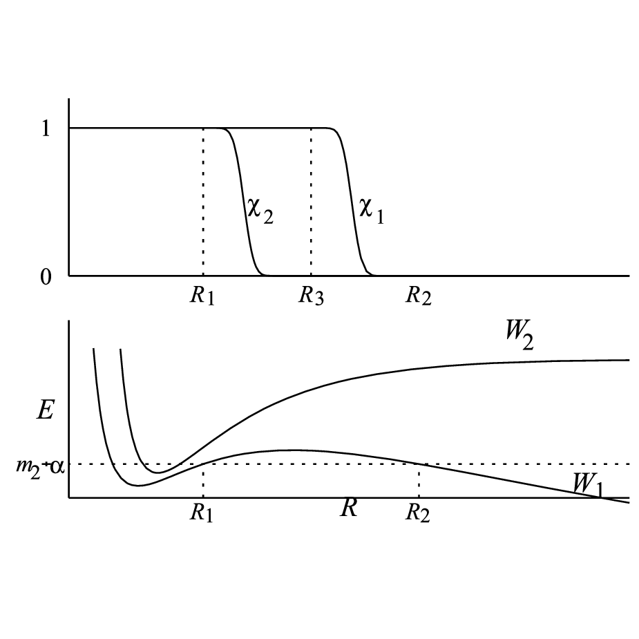
As a consequence, for any λ∈[m1,m2+α]\lambda\in[m_{1},m_{2}+\alpha] (with α>0\alpha>0 small enough), the function W1​(R)−λW_{1}(R)-\lambda presents the shape of a well in an island in the sense of [HeSj2]. Moreover, since we are in dimension one, the complementary of the island (that is, the non compact component of {W1≤λ}\{W_{1}\leq\lambda\}) is automatically non-trapping, and we can adopt the general strategy used in [Ma2] (see also [CMR, FLM]), that consists in taking μ=2​i​h​ln⁡1h\mu=2ih\ln\frac{1}{h} in the definition of the analytic distortion. The function ss used in (14)-(15) can also be assumed to be 0 on a neighborhood of the “greatest” island, defined by {R>0;W1​(R)≥m1}\{R>0\,;W_{1}(R)\geq m_{1}\}. Then, following [FLM], Theorem 2.2 (see also [HeSj2], Proposition 9.6), we first show that the eigenvalues of Pμ♯P_{\mu}^{\sharp} with their real part in [m1,m2+α][m_{1},m_{2}+\alpha], coincide, up to an exponentially small error term, with eigenvalues of the Dirichlet realization PD♯P^{\sharp}_{D} of P0♯P^{\sharp}_{0} on the interval [0,R1,M][0,R_{1,M}].

Proposition 4.2.

Let α>0\alpha>0 small enough, and let 𝒥⊂(0,1]{\mathcal{J}}\subset(0,1], with 0∈𝒥¯0\in\overline{\mathcal{J}}, such that there exists a function a⁡(h)>0a(h)>0 defined for h∈𝒥h\in{\mathcal{J}} and verifying,

For all ε>0,a(h)≥1Cεe−ε/h for h∈𝒥 small enough;\displaystyle\mbox{For all }\varepsilon>0,\,a(h)\geq\frac{1}{C_{\varepsilon}}e^{-\varepsilon/h}\mbox{ for $h\in{\mathcal{J}}$ small enough}; (45)
Sp⁡(PD♯)∩[m2+α−2​a​(h),m2+α+2​a​(h)]=∅.\displaystyle{\rm Sp}(P^{\sharp}_{D})\cap[m_{2}+\alpha-2a(h),m_{2}+\alpha+2a(h)]=\emptyset. (46)

Set,

Ω⁡(h):={z∈ℂ;dist⁡(Rez,[m1,m2+α])<a⁡(h),|Imz|<C−1​h​ln⁡1h},\Omega(h):=\{z\in\mathbb{C}\,;\,{\rm dist}(\mathop{\rm Re}\nolimits z,[m_{1},m_{2}+\alpha])<a(h),\,|\mathop{\rm Im}\nolimits z|<C^{-1}h\ln\frac{1}{h}\},

with C>0C>0 a large enough constant. Then, there exists δ0>0\delta_{0}>0 and a bijection,

b:Sp⁡(PD♯)∩[m1,m2+α]→Sp⁡(Pμ♯)∩Ω⁡(h),b\,:\,{\rm Sp}(P^{\sharp}_{D})\cap[m_{1},m_{2}+\alpha]\rightarrow{\rm Sp}(P_{\mu}^{\sharp})\cap\Omega(h),

such that,

b(λ)−λ=𝒪(e−δ0/h),b(\lambda)-\lambda={\mathcal{O}}(e^{-\delta_{0}/h}),

uniformly for h∈𝒥h\in{\mathcal{J}}.

Remark 4.3.

In our situation, it is well known (see, e.g., [HeRo]) that the distance between two consecutive eigenvalues of the Dirichlet realizations of P1P_{1} and P2P_{2} on (0,R1,M)(0,R_{1,M}), behaves like hh as h→0+h\rightarrow 0_{+}. Then, by slightly moving the parameter α\alpha, it is not difficult to deduce that the previous proposition actually gives a complete description of the spectrum of Pμ♯P_{\mu}^{\sharp} in a neighborhood of [m1,m2+α][m_{1},m_{2}+\alpha], for all sufficiently small values of h>0h>0.

Proof.

At first, we fix a function F=F⁡(R)∈C0∞​((0,R1,M),ℝ+)F=F(R)\in C_{0}^{\infty}((0,R_{1,M});\mathbb{R}_{+}), such that,

inf(0,R1,M](W1+F)>m2+α,\inf_{(0,R_{1,M}]}(W_{1}+F)>m_{2}+\alpha,

and we denote by pj,μ=pj,μ​(R,R∗)p_{j,\mu}=p_{j,\mu}(R,R^{*}) the principal symbol of the operator Pj,μP_{j,\mu}. We also denote by p~j,μ\widetilde{p}_{j,\mu} an almost analytic extension of pj,μp_{j,\mu} (see, e.g., [MeSj]).

Then, using the fact that the whole interval of energy [m1,m2+α][m_{1},m_{2}+\alpha] is non-trapping for the operator P1+FP_{1}+F, we can construct as in [CMR] Section 7 (or [Ma2] Section 4), a real valued function f0=f0​(R,R∗)∈C0∞​((ℝ+\Supp ​F)×ℝ)f_{0}=f_{0}(R,R^{*})\in C_{0}^{\infty}((\mathbb{R}_{+}\backslash\mbox{Supp }F)\times\mathbb{R}), such that, on the set {F(R)+Rep1,μ(R,R∗)∈[m1−δ,m2+α+δ]}\{F(R)+\mathop{\rm Re}\nolimits p_{1,\mu}(R,R^{*})\in[m_{1}-\delta,m_{2}+\alpha+\delta]\} (with δ>0\delta>0 small enough), one has,

−Imp~1,μ(R−hln1h(∂Rf0+i∂R∗f0),R∗−hln1h(∂R∗f0−i∂Rf0))≥δhln1h.-\mathop{\rm Im}\nolimits\widetilde{p}_{1,\mu}\left(R-h\ln\frac{1}{h}\left(\partial_{R}f_{0}+i\partial_{R^{*}}f_{0}\right),R^{*}-h\ln\frac{1}{h}\left(\partial_{R^{*}}f_{0}-i\partial_{R}f_{0}\right)\right)\geq\delta h\ln\frac{1}{h}.

As a consequence (see, e.g., [CMR] Section 7), if z∈ℂz\in\mathbb{C} is such that dist⁡(z,[m1,m2+α])<<h​ln⁡(1/h){\rm dist}(z,[m_{1},m_{2}+\alpha])<<h\ln(1/h), then, the operator P1,μ+F−zP_{1,\mu}+F-z is invertible on L2​(ℝ+)L^{2}(\mathbb{R}_{+}), and its inverse satisfies,

‖h−f0​T​(P1,μ+F−z)−1​u‖L2​(ℝ2)≤C​|h​ln⁡h|−1​‖h−f0​T​u‖L2​(ℝ2),\displaystyle\|h^{-f_{0}}T(P_{1,\mu}+F-z)^{-1}u\|_{L^{2}(\mathbb{R}^{2})}\leq C|h\ln h|^{-1}\|h^{-f_{0}}Tu\|_{L^{2}(\mathbb{R}^{2})}, (47)

where C>0C>0 is a constant, and T:L2​(ℝ+)→L2​(ℝ2)T\,:\,L^{2}(\mathbb{R}_{+})\rightarrow L^{2}(\mathbb{R}^{2}) is the Bargmann tranform, defined by,

T​u​(R,R∗):=12​π​h​∫R′>0ei⁡(R−R′)​R∗/h−(R−R′)2/2​h​u​(R′)​d​R′.Tu(R,R^{*}):=\frac{1}{2\pi h}\int_{R^{\prime}>0}e^{i(R-R^{\prime})R^{*}/h-(R-R^{\prime})^{2}/2h}u(R^{\prime})dR^{\prime}.

Indeed, for any v∈C0∞​(ℝ+)v\in C_{0}^{\infty}(\mathbb{R}_{+}) we have,

‖h−f0​T​v‖L2​(ℝ2)≤C|h​ln⁡h|​‖h−f0​T​(P1,μ+F−z)​v‖L2​(ℝ2),\displaystyle\|h^{-f_{0}}Tv\|_{L^{2}(\mathbb{R}^{2})}\leq\frac{C}{|h\ln h|}\|h^{-f_{0}}T(P_{1,\mu}+F-z)v\|_{L^{2}(\mathbb{R}^{2})}\,, (48)

and, by means of a density argument, we can extend such an estimate to any v∈H2∩H01​(ℝ+)v\in H^{2}\cap H^{1}_{0}(\mathbb{R}_{+}). Then, inequality (47) holds true for the function u=(P1,μ+F−z)​vu=(P_{1,\mu}+F-z)v, which belongs to the space L2​(ℝ+)L^{2}(\mathbb{R}_{+}) and satisfies the Dirichlet condition at R=0R=0.

This means that the operator (P1,μ+F−z)−1(P_{1,\mu}+F-z)^{-1} has a norm 𝒪⁡(|h​ln⁡h|−1){\mathcal{O}}(|h\ln h|^{-1}) if we consider it as acting on the space ℋ=L2​(ℝ+){\mathcal{H}}=L^{2}(\mathbb{R}_{+}) endowed with the norm given by: ‖u‖ℋ:=‖h−f0​T​u‖L2​(ℝ2)\|u\|_{\mathcal{H}}:=\|h^{-f_{0}}Tu\|_{L^{2}(\mathbb{R}^{2})}.

On the other hand, by construction, the operator P2,μ+FP_{2,\mu}+F has a real part greater than m2+αm_{2}+\alpha, and thus, if Rez≤m2+α\mathop{\rm Re}\nolimits z\leq m_{2}+\alpha, we also see that the operator (P2,μ+F−z)−1(P_{2,\mu}+F-z)^{-1} has a uniformly bounded norm when acting on ℋ{\mathcal{H}}.

Then, proceeding as in [HeSj2], Section 9 (see also [FLM], Section 2), we pick up two functions χ1,χ2∈C0∞​((0,R1,M),[0,1])\chi_{1},\chi_{2}\in C_{0}^{\infty}((0,R_{1,M});[0,1]), such that χ1=1\chi_{1}=1 in a neighborhood of Suppχ2{\chi_{2}}, and χ2=1\chi_{2}=1 in a neighborhood of SuppFF. Setting,

Qμ♯:=Pμ♯+F;Rμ♯​(z):=χ1​(PD♯−z)−1​χ2+(Qμ♯−z)−1​(1−χ2),\displaystyle Q_{\mu}^{\sharp}:=P_{\mu}^{\sharp}+F\quad;\quad R_{\mu}^{\sharp}(z):=\chi_{1}(P^{\sharp}_{D}-z)^{-1}\chi_{2}+(Q_{\mu}^{\sharp}-z)^{-1}(1-\chi_{2}), (49)

we see that, if dist⁡(z,Sp⁡(PD♯))≥a⁡(h){\rm dist}(z,{\rm Sp}(P^{\sharp}_{D}))\geq a(h), then ([HeSj2], Formula (9.39) and Proposition 9.8),

(Pμ♯−z)Rμ♯(z)=I+Kμ(z) with ∥Kμ(z)∥ℒ⁡(ℋ)=𝒪(e−2δ/h),(P_{\mu}^{\sharp}-z)R_{\mu}^{\sharp}(z)=I+K_{\mu}(z)\mbox{ with }\|K_{\mu}(z)\|_{{\mathcal{L}}(\mathcal{H})}=\mathcal{O}(e^{-2\delta/h}),

where δ>0\delta>0 is some constant. Therefore, for such values of zz and for hh small enough, we have,

(Pμ♯−z)−1=Rμ♯​(z)​∑j≥0(−Kμ​(z))j,\displaystyle(P_{\mu}^{\sharp}-z)^{-1}=R_{\mu}^{\sharp}(z)\sum_{j\geq 0}(-K_{\mu}(z))^{j}, (50)

and since ‖Rμ♯​(z)‖ℋ=𝒪⁡(h−C)\|R_{\mu}^{\sharp}(z)\|_{\mathcal{H}}=\mathcal{O}(h^{-C}) for some constant C>0C>0, we deduce that, if γ\gamma is a simple oriented loop around Sp⁡(PD♯)∩[m1,m2+α]{\rm Sp}(P^{\sharp}_{D})\cap[m_{1},m_{2}+\alpha] such that dist⁡(γ,Sp⁡(PD♯))≥a⁡(h){\rm dist}(\gamma,{\rm Sp}(P^{\sharp}_{D}))\geq a(h) and dist⁡(γ,[m1,m2+α])<<|h​ln⁡h|{\rm dist}(\gamma,[m_{1},m_{2}+\alpha])<<|h\ln h|, then,

Πμ♯:=12​i​π​∫γ(z−Pμ♯)−1​𝑑z\displaystyle\Pi_{\mu}^{\sharp}:=\frac{1}{2i\pi}\int_{\gamma}(z-P_{\mu}^{\sharp})^{-1}dz =\displaystyle= −12​i​π∫γRμ♯(z)+𝒪(e−δ/h)\displaystyle-\frac{1}{2i\pi}\int_{\gamma}R_{\mu}^{\sharp}(z)+\mathcal{O}(e^{-\delta/h}) (51)
=\displaystyle= 12​i​π∫γχ1(z−PD♯)−1χ2dz+𝒪(e−δ/h).\displaystyle\frac{1}{2i\pi}\int_{\gamma}\chi_{1}(z-P^{\sharp}_{D})^{-1}\chi_{2}dz+\mathcal{O}(e^{-\delta/h}).

Here, we have also used the fact that z↦(Qμ♯−z)−1z\mapsto(Q_{\mu}^{\sharp}-z)^{-1} is holomorphic in the interior of γ\gamma, that can be taken equal to Ω⁡(h)\Omega(h).

Now, since Πμ♯\Pi_{\mu}^{\sharp} is the spectral projector of Pμ♯P_{\mu}^{\sharp} associated with Ω⁡(h)\Omega(h), the corresponding resonances of P♯P^{\sharp} are nothing but the eigenvalues of Pμ♯​Πμ♯P_{\mu}^{\sharp}\Pi_{\mu}^{\sharp} restricted to the range of Πμ♯\Pi_{\mu}^{\sharp}. Moreover, if we set {μ1,…,μm}:=Sp⁡(PD♯)∩[m1,m2+α]\{\mu_{1},\dots,\mu_{m}\}:={\rm Sp}(P^{\sharp}_{D})\cap[m_{1},m_{2}+\alpha], and if we denote by φ1,…,φm\varphi_{1},\dots,\varphi_{m} an orthonormal basis of ⨁j=1mKer⁡(PD♯−μj)\bigoplus_{j=1}^{m}{\rm Ker}(P^{\sharp}_{D}-\mu_{j}), then, by Agmon estimates, we see on (51) (see also [HeSj2],Theorem 9.9 and Corollary 9.10) that the functions Πμ♯​χ1​φj\Pi_{\mu}^{\sharp}\chi_{1}\varphi_{j} (j=1,…,mj=1,\dots,m) form a basis of RanΠμ♯\Pi_{\mu}^{\sharp}, and the matrix of Pμ♯|Ran​Πμ♯P_{\mu}^{\sharp}\left|{}_{{\rm Ran}\Pi_{\mu}^{\sharp}}\right. in this basis, is of the form diag(μ1,…,μm)+𝒪(e−δ/h){\rm diag}(\mu_{1},\dots,\mu_{m})+\mathcal{O}(e^{-\delta/h}). Then, the result follows from standard arguments on the eigenvalues of finite matrices (plus the fact that m=𝒪⁡(h−N0)m=\mathcal{O}(h^{-N_{0}}) for some N0≥1N_{0}\geq 1 constant). ∎

Now, exploiting the fact that both W1​(R1,M)W_{1}(R_{1,M}) and W2​(R1,M)W_{2}(R_{1,M}) are (strictly) greater than m2m_{2}, we consider two functions W~j∈C∞​(ℝ+,ℝ)\widetilde{W}_{j}\in C^{\infty}(\mathbb{R}_{+};\mathbb{R}) (j=1,2j=1,2), such that,

W~j=Wj on [0,R1,M];W~j is constant on [2R1M,+∞);inf[R1,M,+∞)W~j>m2,\widetilde{W}_{j}=W_{j}\mbox{ on }[0,R_{1,M}]\,;\,\widetilde{W}_{j}\mbox{ is constant on }[2R_{1}^{M},+\infty)\,;\,\ \inf_{[R_{1,M},+\infty)}\widetilde{W}_{j}>m_{2},

and we set,

ℳ~0​(R):=(W~1​(R)00W~2​(R)),\widetilde{\mathcal{M}}_{0}(R):=\left(\begin{array}[]{cc}\widetilde{W}_{1}(R)&0\\ 0&\widetilde{W}_{2}(R)\end{array}\right),
P~♯:=h2​DR2+ℳ~0​(R)+h​𝒜0​(R,h​DR),\widetilde{P}^{\sharp}:=h^{2}{\rm D}_{R}^{2}+\widetilde{\mathcal{M}}_{0}(R)+h{\mathcal{A}}_{0}(R,h{\rm D}_{R}),

acting on the space ℋ♯{\mathcal{H}}^{\sharp}. That is, P~♯\widetilde{P}^{\sharp} is obtained form P♯P^{\sharp} by substituting W~1,W~2\widetilde{W}_{1},\widetilde{W}_{2} to W1,W2W_{1},W_{2}. Then, the same arguments used in Proposition 4.2 (and actually simpler, since both operators are self-adjoints) show that, under the same conditions, the spectrum of PD♯P^{\sharp}_{D} and the spectrum of P~♯\widetilde{P}^{\sharp} coincide in [m1,m1+α+a⁡(h)][m_{1},m_{1}+\alpha+a(h)], up to some exponentially small error-terms. Therefore, in order to know the resonances of P♯P^{\sharp} in Ω⁡(h)\Omega(h) (up to those exponentially small error-terms), it is sufficient to study the eigenvalues λ\lambda of the self-adjoint P~♯\widetilde{P}^{\sharp} in [m1,m1+α+a⁡(h)][m_{1},m_{1}+\alpha+a(h)].

For j=1,2j=1,2, we set,

P~j:=h2​DR2+W~j,\widetilde{P}_{j}:=h^{2}D_{R}^{2}+\widetilde{W}_{j},

acting on L2​(ℝ+,d​R)L^{2}(\mathbb{R}^{+};dR) with Dirichlet condition at R=0R=0, and we consider separately two different cases.

4.1. Case 1: λ≤(m2−α)\lambda\leq(m_{2}-\alpha)

In that case, the operator P~2−λ\widetilde{P}_{2}-\lambda is invertible, with a uniformly bounded inverse, and the equation,

P~♯​φ=λ​φ,φ=(φ1φ2),\displaystyle\widetilde{P}^{\sharp}\varphi=\lambda\varphi,\quad\varphi=\left(\begin{array}[]{c}\varphi_{1}\\ \varphi_{2}\end{array}\right),

can be re-written as,

φ2=−h​(P~2−λ)−1​A0∗​φ1;\displaystyle\varphi_{2}=-h(\widetilde{P}_{2}-\lambda)^{-1}A_{0}^{*}\varphi_{1};
[P~1−h2​A0​(P~2−λ)−1​A0∗]​φ1=λ​φ1.\displaystyle\left[\widetilde{P}_{1}-h^{2}A_{0}(\widetilde{P}_{2}-\lambda)^{-1}A_{0}^{*}\right]\varphi_{1}=\lambda\varphi_{1}.

Thus, the eigenvalues λ\lambda are given by the equation,

λ=f~k​(λ),\displaystyle\lambda=\widetilde{f}_{k}(\lambda), (55)

where the f~k​(λ)\widetilde{f}_{k}(\lambda)’s are the eigenvalues of P^1​(λ):=P~1−h2​A0​(P~2−λ)−1​A0∗\hat{P}_{1}(\lambda):=\widetilde{P}_{1}-h^{2}A_{0}(\widetilde{P}_{2}-\lambda)^{-1}A_{0}^{*}.

Writing,

P^1​(λ)−z=(1−h2​A0​(P~2−λ)−1​A0∗​(P~1−z)−1)​(P~1−z),\hat{P}_{1}(\lambda)-z=(1-h^{2}A_{0}(\widetilde{P}_{2}-\lambda)^{-1}A_{0}^{*}(\widetilde{P}_{1}-z)^{-1})(\widetilde{P}_{1}-z),

and observing that, for z∉Sp​(P~1)z\notin\mbox{\rm Sp}(\widetilde{P}_{1}), A0∗​(P~1−z)−1A_{0}^{*}(\widetilde{P}_{1}-z)^{-1} is bounded and has a norm 𝒪⁡(dist ​(z,Sp​(P~1))−1)\mathcal{O}(\mbox{\rm dist }(z,\mbox{\rm Sp}(\widetilde{P}_{1}))^{-1}), we conclude that, if dist ​(z,Sp​(P~1))>>h2\mbox{\rm dist }(z,\mbox{\rm Sp}(\widetilde{P}_{1}))>>h^{2}, then P^1​(λ)−z\hat{P}_{1}(\lambda)-z is invertible, and its inverse satisfies,

(P^1​(λ)−z)−1=(P~1−z)−1​(1+𝒪⁡(h2/dist ​(z,Sp​(P~1)))).(\hat{P}_{1}(\lambda)-z)^{-1}=(\widetilde{P}_{1}-z)^{-1}(1+\mathcal{O}(h^{2}/\mbox{\rm dist }(z,\mbox{\rm Sp}(\widetilde{P}_{1})))).

Differentiating with respect to λ\lambda, we also obtain,

dd​λ​(P^1​(λ)−z)−1=(P~1−z)−1​𝒪​(h2/dist ​(z,Sp​(P~1)))=𝒪⁡(h2/dist ​(z,Sp​(P~1))2).\frac{d}{d\lambda}(\hat{P}_{1}(\lambda)-z)^{-1}=(\widetilde{P}_{1}-z)^{-1}\mathcal{O}(h^{2}/\mbox{\rm dist }(z,\mbox{\rm Sp}(\widetilde{P}_{1})))=\mathcal{O}(h^{2}/\mbox{\rm dist }(z,\mbox{\rm Sp}(\widetilde{P}_{1}))^{2}).

Then, using the fact that, under the non degenerate condition discussed in Remark 4.1, the eigenvalues E1,kE_{1,k} (k≥1k\geq 1) of P~1\widetilde{P}_{1} are distant at least of order hh between each other, for each of them we can define the projection,

Π^1​(λ):=12​i​π​∫γk(z−P^1​(λ))−1​𝑑z,\hat{\Pi}_{1}(\lambda):=\frac{1}{2i\pi}\int_{\gamma_{k}}(z-\hat{P}_{1}(\lambda))^{-1}dz,

where γk\gamma_{k} is a complex oriented simple circle centered at Ek1E_{k}^{1} of radius δ​h\delta h with δ>0\delta>0 small enough. Applying standard regular perturbation theory, we easily conclude that the kk-th eigenvalue of f~k​(λ)\widetilde{f}_{k}(\lambda) of P^1​(λ)\hat{P}_{1}(\lambda) satisfies,

fk​(λ)=E1,k+𝒪⁡(h2);d​fkd​λ​(λ)=𝒪⁡(h),\displaystyle f_{k}(\lambda)=E_{1,k}+\mathcal{O}(h^{2})\quad;\quad\frac{df_{k}}{d\lambda}(\lambda)=\mathcal{O}(h), (56)

uniformly with respect to hh small enough, k≥1k\geq 1 such that Ek1≤m2−12​αE_{k}^{1}\leq m_{2}-\frac{1}{2}\alpha, and λ≤m2−α\lambda\leq m_{2}-\alpha.

By the implicit function theorem, it follows that the kk-th eigenvalue λk\lambda_{k} of P~♯\widetilde{P}^{\sharp} satisfies,

λk=E1,k+𝒪⁡(h2),\lambda_{k}=E_{1,k}+\mathcal{O}(h^{2}),

uniformly with respect to h>0h>0 small enough and to k=𝒪⁡(h−1)k=\mathcal{O}(h^{-1}), such that E1,k≤m2−12​αE_{1,k}\leq m_{2}-\frac{1}{2}\alpha.

4.2. Case 2: λ∈[m2−α,m2+α]\lambda\in[m_{2}-\alpha,m_{2}+\alpha] with α>0\alpha>0 small enough

We denote by ϕ1,…,ϕn\phi_{1},\dots,\phi_{n} an orthonormal family of eigenfunctions of P~1\widetilde{P}_{1} with eigenvalues in the interval [m2−2​α,m2+2​α][m_{2}-2\alpha,\,m_{2}+2\alpha] and by ψ1,…,ψm\psi_{1},\dots,\psi_{m} an orthonormal family of eigenfunctions of P~2\widetilde{P}_{2} with eigenvalues in the interval [m2,m2+2​α][m_{2},\,m_{2}+2\alpha] (in particular, we have n,m=𝒪⁡(h−1)n,m=\mathcal{O}(h^{-1})).

For α⊕β∈ℂn⊕ℂm\alpha\oplus\beta\in\mathbb{C}^{n}\oplus\mathbb{C}^{m}, we set,

R−​(α⊕β):=α⋅ϕ⊕β⋅ψ∈ℋ♯,R_{-}(\alpha\oplus\beta):=\alpha\cdot\phi\oplus\beta\cdot\psi\in\mathcal{H}^{\sharp},

where we have used the notation,

α⋅ϕ:=∑k=1nαk​ϕk;β⋅ψ:=∑ℓ=1mβℓ​ψℓ.\alpha\cdot\phi:=\sum_{k=1}^{n}\alpha_{k}\phi_{k}\quad;\quad\beta\cdot\psi:=\sum_{\ell=1}^{m}\beta_{\ell}\psi_{\ell}.

We also denote by R+R_{+} the adjoint of R−R_{-}, given by,

R+​(u⊕v)=(⟨u,ϕk⟩)1≤k≤n⊕(⟨v,ψℓ⟩)1≤ℓ≤m.R_{+}(u\oplus v)=(\langle u,\phi_{k}\rangle)_{1\leq k\leq n}\oplus(\langle v,\psi_{\ell}\rangle)_{1\leq\ell\leq m}.

Then, we consider the operator valued matrix,

G⁡(λ)=(P~♯−λR−R+0),\displaystyle G(\lambda)=\left(\begin{array}[]{cc}\widetilde{P}^{\sharp}-\lambda&R_{-}\\ R_{+}&0\end{array}\right),

on

ℋ♯⊕ℂn⊕ℂm,\displaystyle\mathcal{H}^{\sharp}\oplus\mathbb{C}^{n}\oplus\mathbb{C}^{m},

with domain (H2∩H01)​(ℝ+)⊕(H2∩H01)​(ℝ+)⊕ℂn⊕ℂm(H^{2}\cap H^{1}_{0})(\mathbb{R}_{+})\oplus(H^{2}\cap H^{1}_{0})(\mathbb{R}_{+})\oplus\mathbb{C}^{n}\oplus\mathbb{C}^{m}, and we want to know whether G⁡(λ)G(\lambda) is invertible.

We denote by Π1\Pi_{1} and Π2\Pi_{2} the orthogonal projections on the subspaces SnS_{n} and SmS_{m} of L2​(ℝ+)L^{2}(\mathbb{R}_{+}) spanned by the eigenfunctions ϕ1,…,ϕn\phi_{1},\dots,\phi_{n} and ψ1,…,ψm\psi_{1},\dots,\psi_{m} respectively, and we set,

Π:=(Π100Π2),Π⊥=(Π1⊥00Π2⊥):=(1−Π1001−Π2).\Pi:=\left(\begin{array}[]{cc}\Pi_{1}&0\\ 0&\Pi_{2}\end{array}\right)\,;\,\Pi^{\bot}=\left(\begin{array}[]{cc}\Pi_{1}^{\bot}&0\\ 0&\Pi_{2}^{\bot}\end{array}\right):=\left(\begin{array}[]{cc}1-\Pi_{1}&0\\ 0&1-\Pi_{2}\end{array}\right).

We first prove,

Lemma 4.4.

For λ∈[m2−α,m2+α]\lambda\in[m_{2}-\alpha,m_{2}+\alpha], the operator Π⊥​P~♯​Π⊥−λ=:P~⊥♯−λ\Pi^{\bot}\widetilde{P}^{\sharp}\Pi^{\bot}-\lambda=:\widetilde{P}^{\sharp}_{\bot}-\lambda is invertible on the range Ran ​Π⊥\mbox{Ran }\Pi^{\bot} of Π⊥\Pi^{\bot}, and its inverse (P~⊥♯−λ)−1(\widetilde{P}^{\sharp}_{\bot}-\lambda)^{-1} is uniformly bounded.

Proof.

We have,

Π⊥​(P~♯−λ)​Π⊥=(Π1⊥​(P~1−λ)​Π1⊥h​Π1⊥​A0​Π2⊥h​Π2⊥​A0∗​Π1⊥Π2⊥​(P~2−λ)​Π2⊥),\Pi^{\bot}(\widetilde{P}^{\sharp}-\lambda)\Pi^{\bot}=\left(\begin{array}[]{cc}\Pi_{1}^{\bot}(\widetilde{P}_{1}-\lambda)\Pi_{1}^{\bot}&h\Pi_{1}^{\bot}A_{0}\Pi_{2}^{\bot}\\ h\Pi_{2}^{\bot}A_{0}^{*}\Pi_{1}^{\bot}&\Pi_{2}^{\bot}(\widetilde{P}_{2}-\lambda)\Pi_{2}^{\bot}\end{array}\right),

and, denoting by P~j⊥\widetilde{P}_{j}^{\bot} the restriction of P~j\widetilde{P}_{j} to Ran ​Πj⊥\mbox{Ran }\Pi_{j}^{\bot}, we know that P~j⊥−λ\widetilde{P}_{j}^{\bot}-\lambda is invertible, and it is standard to show that its inverse is uniformly bounded from Ran ​Πj⊥\mbox{Ran }\Pi_{j}^{\bot} to Ran ​Πj⊥∩(H2∩H10)​(ℝ+)\mbox{Ran }\Pi_{j}^{\bot}\cap(H^{2}\cap H_{1}^{0})(\mathbb{R}_{+}), if one takes the hh-dependent norm on H2​(ℝ+)H^{2}(\mathbb{R}_{+}) defined by: ‖u‖H22:=‖h2​Δ​u‖L22+‖u‖L22\|u\|^{2}_{H^{2}}:=\|h^{2}\Delta u\|_{L^{2}}^{2}+\|u\|_{L^{2}}^{2}. As a consequence, A0​Π2⊥​(P~2⊥−λ)−1​Π2⊥A_{0}\Pi_{2}^{\bot}(\widetilde{P}_{2}^{\bot}-\lambda)^{-1}\Pi_{2}^{\bot} and A0​Π1⊥​(P~1⊥−λ)−1​Π1⊥A_{0}\Pi_{1}^{\bot}(\widetilde{P}_{1}^{\bot}-\lambda)^{-1}\Pi_{1}^{\bot} are uniformly bounded on L2​(ℝ+)L^{2}(\mathbb{R}_{+}) (together with their adjoint), and we find,

Π⊥​(P~♯−λ)​Π⊥​((P~1⊥−λ)−100(P~2⊥−λ)−1)​Π⊥=Π⊥​(1+𝒪⁡(h))​Π⊥;\Pi^{\bot}(\widetilde{P}^{\sharp}-\lambda)\Pi^{\bot}\left(\begin{array}[]{cc}(\widetilde{P}_{1}^{\bot}-\lambda)^{-1}&0\\ 0&(\widetilde{P}_{2}^{\bot}-\lambda)^{-1}\end{array}\right)\Pi^{\bot}=\Pi^{\bot}(1+\mathcal{O}(h))\Pi^{\bot};
Π⊥​((P~1⊥−λ)−100(P~2⊥−λ)−1)​Π⊥​(P~♯−λ)​Π⊥=Π⊥​(1+𝒪⁡(h))​Π⊥.\Pi^{\bot}\left(\begin{array}[]{cc}(\widetilde{P}_{1}^{\bot}-\lambda)^{-1}&0\\ 0&(\widetilde{P}_{2}^{\bot}-\lambda)^{-1}\end{array}\right)\Pi^{\bot}(\widetilde{P}^{\sharp}-\lambda)\Pi^{\bot}=\Pi^{\bot}(1+\mathcal{O}(h))\Pi^{\bot}.

Thus, the result follows by taking the restriction to Ran ​Π⊥\mbox{Ran }\Pi^{\bot}, and by using the Neumann series in order to inverse Π⊥(1+𝒪(h))Π⊥|=Ran ​Π⊥(1+Π⊥𝒪(h))|Ran ​Π⊥\Pi^{\bot}(1+\mathcal{O}(h))\Pi^{\bot}\left|{}_{\mbox{Ran }\Pi^{\bot}}\right.=(1+\Pi^{\bot}\mathcal{O}(h))\left|{}_{\mbox{Ran }\Pi^{\bot}}\right.. ∎

Using the previous lemma, it is easy to show that G⁡(λ)G(\lambda) is invertible, and to check that its inverse is given by,

G​(λ)−1=(Π⊥​(P~⊥♯−λ)−1​Π⊥(1−Π⊥​(P~⊥♯−λ)−1​Π⊥​P~♯)​R−R+​(1−P~♯​Π⊥​(P~⊥♯−λ)−1​Π⊥)λ−Q⁡(λ))G(\lambda)^{-1}=\left(\begin{array}[]{cc}\Pi^{\bot}(\widetilde{P}^{\sharp}_{\bot}-\lambda)^{-1}\Pi^{\bot}&(1-\Pi^{\bot}(\widetilde{P}^{\sharp}_{\bot}-\lambda)^{-1}\Pi^{\bot}\widetilde{P}^{\sharp})R_{-}\\ R_{+}(1-\widetilde{P}^{\sharp}\Pi^{\bot}(\widetilde{P}^{\sharp}_{\bot}-\lambda)^{-1}\Pi^{\bot})&\lambda-Q(\lambda)\end{array}\right)

with,

Q⁡(λ):=R+​P~♯​(1−Π⊥​(P~⊥♯−λ)−1​Π⊥​P~♯)​R−.\displaystyle Q(\lambda):=R_{+}\widetilde{P}^{\sharp}(1-\Pi^{\bot}(\widetilde{P}^{\sharp}_{\bot}-\lambda)^{-1}\Pi^{\bot}\widetilde{P}^{\sharp})R_{-}. (58)

In particular, Q⁡(λ)Q(\lambda) is an (n+m)×(n+m)(n+m)\times(n+m) matrix with n,m=𝒪⁡(h−1)n,m=\mathcal{O}(h^{-1}).

Proposition 4.5.

The matrix Q⁡(λ)Q(\lambda) satisfies,

Q⁡(λ)=diag ​(E1,1,…,E1,n,E2,1,…,E2,m)+S⁡(λ),\displaystyle Q(\lambda)=\mbox{\rm diag }(E_{1,1},\dots,E_{1,n},E_{2,1},\dots,E_{2,m})+S(\lambda),

where E1,j,E2,k∈[m2−2​α,m2+2​α]E_{1,j},E_{2,k}\in[m_{2}-2\alpha,\,m_{2}+2\alpha] are the eigenvalues associated with ϕj\phi_{j} and ψk\psi_{k}, respectively, and with,

‖S⁡(λ)‖+‖dd​λ​S​(λ)‖=𝒪⁡(h2),\|S(\lambda)\|+\|\frac{d}{d\lambda}S(\lambda)\|=\mathcal{O}(h^{2}),

in the sense of the norm of operators on ℂn+m\mathbb{C}^{n+m}, and uniformly with respect to h>0h>0 small enough and n,m=𝒪⁡(h−1)n,m=\mathcal{O}(h^{-1}).

Proof.

Since R+​Π⊥=0R_{+}\Pi^{\bot}=0 and Π⊥​R−=0\Pi^{\bot}R_{-}=0, by (58), we have,

Q⁡(λ)=R+​P~♯​R−−R+​Π​P~♯​Π⊥​(P~⊥♯−λ)−1​Π⊥​P~♯​Π​R−,\displaystyle Q(\lambda)=R_{+}\widetilde{P}^{\sharp}R_{-}-R_{+}\Pi\widetilde{P}^{\sharp}\Pi^{\bot}(\widetilde{P}^{\sharp}_{\bot}-\lambda)^{-1}\Pi^{\bot}\widetilde{P}^{\sharp}\Pi R_{-}, (59)
dd​λ​Q​(λ)=R+​Π​P~♯​Π⊥​(P~⊥♯−λ)−2​Π⊥​P~♯​Π​R−,\displaystyle\frac{d}{d\lambda}Q(\lambda)=R_{+}\Pi\widetilde{P}^{\sharp}\Pi^{\bot}(\widetilde{P}^{\sharp}_{\bot}-\lambda)^{-2}\Pi^{\bot}\widetilde{P}^{\sharp}\Pi R_{-}, (60)

and, since Πj​P~j​Πj⊥=0\Pi_{j}\widetilde{P}_{j}\Pi_{j}^{\bot}=0 (j=1,2j=1,2),

Π​P~♯​Π⊥=(0h​Π1​A0​Π2⊥h​Π2​A0∗​Π1⊥0).\displaystyle\Pi\widetilde{P}^{\sharp}\Pi^{\bot}=\left(\begin{array}[]{cc}0&h\Pi_{1}A_{0}\Pi_{2}^{\bot}\\ h\Pi_{2}A_{0}^{*}\Pi_{1}^{\bot}&0\end{array}\right).

Moreover, using that ‖P~j​Πj‖ℒ⁡(L2)≤|m2|+2​α\|\widetilde{P}_{j}\Pi_{j}\|_{{\mathcal{L}}(L^{2})}\leq|m_{2}|+2\alpha and the ellipticity of P~j\widetilde{P}_{j}, it is easy to see that both A0∗​Π1A_{0}^{*}\Pi_{1} and A0​Π2A_{0}\Pi_{2} are uniformly bounded, thus so are their adjoints Π1​A0\Pi_{1}A_{0} and Π2​A0∗\Pi_{2}A_{0}^{*}, and we deduce from (59)-(4.2) (plus the fact that ‖R±‖≤1\|R_{\pm}\|\leq 1),

Q⁡(λ)=R+​P~♯​R−+𝒪⁡(h2);dd​λ​Q​(λ)=𝒪⁡(h2).\displaystyle Q(\lambda)=R_{+}\widetilde{P}^{\sharp}R_{-}+\mathcal{O}(h^{2})\quad;\quad\frac{d}{d\lambda}Q(\lambda)=\mathcal{O}(h^{2}). (64)

Therefore, in order to complete the proof of Proposition 4.5, it is enough to show,

Lemma 4.6.

For all N≥0N\geq 0, there exists a constant CN>0C_{N}>0 such that, for all j∈{1,…,n}j\in\{1,\dots,n\} and k∈{1,…,m}k\in\{1,\dots,m\}, one has,

|⟨A0​ϕj,ψk⟩|+|⟨A0​ψk,ϕj⟩|≤CN​hN.|\langle A_{0}\phi_{j},\psi_{k}\rangle|+|\langle A_{0}\psi_{k},\phi_{j}\rangle|\leq C_{N}h^{N}.
Proof.

We use the equations,

(P~1−E1,j)​ϕj=0;(P~2−E2,k)​ψk=0.\displaystyle(\widetilde{P}_{1}-E_{1,j})\phi_{j}=0\quad;\quad(\widetilde{P}_{2}-E_{2,k})\psi_{k}=0. (65)

At first, we observe that, for RR close enough to 0 (say, 0<R<r00<R<r_{0}), and RR large enough (say, R>R0R>R_{0}), both W1​(R)−E1,jW_{1}(R)-E_{1,j} and W2​(R)−E2,kW_{2}(R)-E_{2,k} remain greater than some fix constant C>0C>0. Therefore, by standard Agmon estimates (see, e.g., [Ma1], Chapter 3, exercise 8), it is easy to show that, for hh small enough,

∥ϕj∥Hs​((0,r0)∪(R0,+∞))+∥ψk∥Hs​((0,r0)∪(R0,+∞))≤e−c0/h,\displaystyle\|\phi_{j}\|_{H^{s}((0,r_{0})\cup(R_{0},+\infty))}+\|\psi_{k}\|_{H^{s}((0,r_{0})\cup(R_{0},+\infty))}\leq e^{-c_{0}/h}, (66)

where the positive constant c0c_{0} does not depend on j,k=𝒪⁡(h−1)j,k=\mathcal{O}(h^{-1}), and s≥0s\geq 0 is arbitrary.

For ℓ=1,2\ell=1,2, we set,

Σℓ:={(R,R∗)∈ℝ+×ℝ;p~ℓ​(R,R∗)∈[m2−2​α,m2+2​α]}\Sigma_{\ell}:=\{(R,R^{*})\in\mathbb{R}_{+}\times\mathbb{R}\,;\,\widetilde{p}_{\ell}(R,R^{*})\in[m_{2}-2\alpha,m_{2}+2\alpha]\}

(where we have used the notation p~ℓ​(R,R∗):=(R∗)2+W~ℓ​(R)\widetilde{p}_{\ell}(R,R^{*}):=(R^{*})^{2}+\widetilde{W}_{\ell}(R)), and we chose χℓ∈C0∞​((12​r0,2​R0)×ℝ)\chi_{\ell}\in C_{0}^{\infty}((\frac{1}{2}r_{0},2R_{0})\times\mathbb{R}), supported near Σℓ\Sigma_{\ell}, such that χℓ=1\chi_{\ell}=1 in a neighborhood of Σℓ\Sigma_{\ell}. We also fix χ0=χ0​(R)∈C0∞​(12​r0,2​R0)\chi_{0}=\chi_{0}(R)\in C_{0}^{\infty}(\frac{1}{2}r_{0},2R_{0}), such that χ0=1\chi_{0}=1 near [r0,R0][r_{0},R_{0}].

Then, using standard pseudodifferential calculus, for any E∈[m2−2​α,m2+2​α]E\in[m_{2}-2\alpha,m_{2}+2\alpha] one can construct a symbol qℓ​(E)=qℓ​(E,R,R∗,h)∈S⁡(⟨R∗⟩−2)q_{\ell}(E)=q_{\ell}(E,R,R^{*};h)\in S(\langle R^{*}\rangle^{-2}), supported in (12​r0,2​R0)×ℝ(\frac{1}{2}r_{0},2R_{0})\times\mathbb{R} and depending smoothly on EE, such that,

qℓ​(E)​#​(p~ℓ−E)​(R,R∗)∼χ0​(R)​(1−χℓ​(R,R∗)).\displaystyle q_{\ell}(E)\#(\widetilde{p}_{\ell}-E)(R,R^{*})\sim\chi_{0}(R)(1-\chi_{\ell}(R,R^{*})). (67)

Here, #\# stands for the Weyl-composition of symbols, and the asymptotic equivalence holds in S⁡(1)S(1), uniformly with respect to E∈[m2−2​α,m2+2​α]E\in[m_{2}-2\alpha,m_{2}+2\alpha] (see, e.g., [Ma1]). Then, first multiplying (65) by χ0\chi_{0}, then, commuting χ0\chi_{0} and P~j\widetilde{P}_{j}, and finally applying the usual Weyl-quantization of qℓ​(E)q_{\ell}(E) (with E=E1,j,E2,kE=E_{1,j},E_{2,k}, respectively), we deduce from (65), (66) and (67),

‖(1−χ1​(R,h​DR))​χ0​ϕj‖Hs=𝒪⁡(h∞);\displaystyle\|(1-\chi_{1}(R,hD_{R}))\chi_{0}\phi_{j}\|_{H^{s}}=\mathcal{O}(h^{\infty}); (68)
‖(1−χ2​(R,h​DR))​χ0​ψk‖Hs=𝒪⁡(h∞)\displaystyle\|(1-\chi_{2}(R,hD_{R}))\chi_{0}\psi_{k}\|_{H^{s}}=\mathcal{O}(h^{\infty}) (69)

uniformly with respect to j,kj,k (here, χℓ​(R,h​DR)\chi_{\ell}(R,hD_{R}) stands for the Weyl-quantization of χℓ\chi_{\ell}).

Now, if α\alpha is taken sufficiently small, the sets Σ1\Sigma_{1} and Σ2\Sigma_{2} are disjoints, and thus the supports of χ1\chi_{1} and χ2\chi_{2} can be taken disjoints, too. Since they are also disjoints from Supp ​(1−χ0)\mbox{\rm Supp }(1-\chi_{0}), one can find χ3∈C∞​(ℝ+×ℝ,[0,1])\chi_{3}\in C^{\infty}(\mathbb{R}_{+}\times\mathbb{R};[0,1]), supported in (12​r0,2​R0)×ℝ(\frac{1}{2}r_{0},2R_{0})\times\mathbb{R}, such that the family {χ1,χ2,χ3}\{\chi_{1},\chi_{2},\chi_{3}\} forms a partition of unity on Supp ​χ0×ℝ\mbox{\rm Supp }\chi_{0}\times\mathbb{R}. In particular, on L2​(ℝ+)L^{2}(\mathbb{R}_{+}), one has,

1−χ0​(R)+∑ℓ=13χℓ​(R,h​DR)​χ0​(R)=I,1-\chi_{0}(R)+\sum_{\ell=1}^{3}\chi_{\ell}(R,hD_{R})\chi_{0}(R)=I,

and now, it is clear that, inserting this microlocal partition of unity in the products ⟨A0​ϕj,ψk⟩\langle A_{0}\phi_{j},\psi_{k}\rangle and ⟨A0​ψk,ϕj⟩\langle A_{0}\psi_{k},\phi_{j}\rangle, the estimates (66), (68) and (69) give the required result. ∎

Remark 4.7.

Actually, following more precisely the construction of H~eμ\widetilde{H}_{e}^{\mu} made in Section 4, one can prove that the functions W~j\widetilde{W}_{j} (j=1,2j=1,2) and a0a_{0} depend in an analytic way of RR in a neighborhood of the relevant classically allowed region {W~1(R)≤m2+2α}\{\widetilde{W}_{1}(R)\leq m_{2}+2\alpha\}. As a consequence, one can use the standard microlocal analytic techniques in this region (see, e.g., [Sj, Ma1]), and obtain the existence of a constant c0>0c_{0}>0 (independent of j,kj,k), such that,

|⟨A0ϕj,ψk⟩|+|⟨A0ψk,ϕj⟩|≤e−c0/h.|\langle A_{0}\phi_{j},\psi_{k}\rangle|+|\langle A_{0}\psi_{k},\phi_{j}\rangle|\leq e^{-c_{0}/h}.

Completion of the proof of the proposition: Since the matrix,

R+​P~♯​R−−diag ​(E1,1,…,E2,m)=(0(⟨A0ψk,ϕj)(⟨A0∗​ϕj,ψk⟩)0)R_{+}\widetilde{P}^{\sharp}R_{-}-\mbox{\rm diag }(E_{1,1},\dots,E_{2,m})=\left(\begin{array}[]{cc}0&(\langle A_{0}\psi_{k},\phi_{j})\\ (\langle A_{0}^{*}\phi_{j},\psi_{k}\rangle)&0\end{array}\right)

is of size 𝒪⁡(h−1)\mathcal{O}(h^{-1}), Lemma 4.6 implies that it has a norm 𝒪⁡(h∞)\mathcal{O}(h^{\infty}) on ℂn+m\mathbb{C}^{n+m}, uniformly with respect to n,mn,m. Thus, Proposition 4.5 is a consequence of (64). ∎

By the Min-Max principle, it results from Proposition 4.5 that, for λ∈[m2−α,m2+α]\lambda\in[m_{2}-\alpha,m_{2}+\alpha], the eigenvalues g1​(λ),…,gm+n​(λ)g_{1}(\lambda),\dots,g_{m+n}(\lambda) of Q⁡(λ)Q(\lambda) satisfy,

{g1​(λ),…,gm+n​(λ)}={E1,1,…,E1,n,E2,1,…,E2,m}+𝒪⁡(h2);\displaystyle\{g_{1}(\lambda),\dots,g_{m+n}(\lambda)\}=\{E_{1,1},\dots,E_{1,n},E_{2,1},\dots,E_{2,m}\}+\mathcal{O}(h^{2});
λ↦gℓ​(λ)​ is Lipschitz continuous ​(ℓ=1,…​n+m);\displaystyle\lambda\mapsto g_{\ell}(\lambda)\mbox{ is Lipschitz continuous }(\ell=1,\dots n+m);
|d​gℓd​λ|=𝒪⁡(h2)​a.e.(k=1,…​n+m).\displaystyle\left|\frac{dg_{\ell}}{d\lambda}\right|=\mathcal{O}(h^{2})\,\,a.e.\,\,(k=1,\dots n+m). (70)

Note that the values E1,1,…,E1,nE_{1,1},\dots,E_{1,n} are at a distance of order hh from each other, and the same is true for the values E2,1,…,E2,mE_{2,1},\dots,E_{2,m}. So the only problem that may appear in the computation of gℓ​(λ)g_{\ell}(\lambda) is when, along some sequence h=hj→0+h=h_{j}\rightarrow 0_{+}, two values E1,jE_{1,j} and E2,kE_{2,k} become closer than 𝒪⁡(h2)\mathcal{O}(h^{2}). But, in that case, the two corresponding values of gℓ​(λ)g_{\ell}(\lambda) are given by,

gℓ​(λ)=12​(E1,j+E2,k+h2​r1±(E1,j−E2,k+h2​r2)2+h4​r32),\displaystyle g_{\ell}(\lambda)=\frac{1}{2}\left(E_{1,j}+E_{2,k}+h^{2}r_{1}\pm\sqrt{(E_{1,j}-E_{2,k}+h^{2}r_{2})^{2}+h^{4}r_{3}^{2}}\right), (71)

with rt=rt​(λ)r_{t}=r_{t}(\lambda) smooth, rt=𝒪⁡(1)r_{t}=\mathcal{O}(1), d​rt/d​λ=𝒪⁡(1)dr_{t}/d\lambda=\mathcal{O}(1) (t=1,2,3t=1,2,3). Thus, actually, a correct (hh-depending) indexing of the gℓg_{\ell}’s make them smooth functions of λ\lambda, and then (70) becomes true everywhere.

Anyway, (70) is enough to insure that all the values of λ∈[m2−α,m2+α]\lambda\in[m_{2}-\alpha,m_{2}+\alpha] such that λ∈Sp ​Q​(λ)\lambda\in\mbox{\rm Sp }Q(\lambda) verify,

dist ​(λ,{E1,1,…,E1,n,E2,1,…,E2,m})=𝒪⁡(h2),\mbox{\rm dist }(\lambda,\{E_{1,1},\dots,E_{1,n},E_{2,1},\dots,E_{2,m}\})=\mathcal{O}(h^{2}),

and, conversely, at any E∈{E1,1,…,E1,n,E2,1,…,E2,m}∩[m2−α+C​h2,m2+α−C​h2]E\in\{E_{1,1},\dots,E_{1,n},E_{2,1},\dots,E_{2,m}\}\cap[m_{2}-\alpha+Ch^{2},m_{2}+\alpha-Ch^{2}] (C>0C>0 large enough), can be associated a unique λ∈[m2−α,m2+α]\lambda\in[m_{2}-\alpha,m_{2}+\alpha] such that λ∈Sp ​Q​(λ)\lambda\in\mbox{\rm Sp }Q(\lambda).

Finally, using the fact that, by construction, the eigenvalues of P~♯\widetilde{P}^{\sharp} that lie in [m2−α,m2+α][m_{2}-\alpha,m_{2}+\alpha] coincide with the solutions there of λ∈Sp ​Q​(λ)\lambda\in\mbox{\rm Sp }Q(\lambda), and summing up with the results of Subsection 4.1 and Proposition 4.2, we finally obtain,

Theorem 4.8.

For h>0h>0 small enough the resonances of P♯P^{\sharp} with real part in [m1,m2+α][m_{1},m_{2}+\alpha] and with imaginary part <<|hlnh|<<|h\ln h|, coincide, up to 𝒪⁡(h2)\mathcal{O}(h^{2}) error-terms, with eigenvalues of the Dirichlet realizations of P1P_{1} and P2P_{2} on (0,R1,M)(0,R_{1,M}), where R1,M>0R_{1,M}>0 is the point where W1W_{1} admits a local maximum with value greater than m2m_{2}.

5. Comparison between the spectrum of the operators Pμ♯P_{\mu}^{\sharp} and H~μ0\widetilde{H}_{\mu}^{0}

Here we prove,

Proposition 5.1.

Let α>0\alpha>0 fixed small enough, and let 𝒥⊂(0,1]{\mathcal{J}}\subset(0,1], with 0∈𝒥¯0\in\overline{\mathcal{J}}, such that there exists δ>0\delta>0 such that,

Sp⁡(PD♯)∩[m2+α−2​δ​h,m2+α+2​δ​h]=∅.\displaystyle{\rm Sp}(P^{\sharp}_{D})\cap[m_{2}+\alpha-2\delta h,m_{2}+\alpha+2\delta h]=\emptyset. (72)

Set,

Ω⁡(h):={z∈ℂ;dist⁡(Rez,[m1,m2+α])<δ​h,|Imz|<C−1​h​ln⁡1h},\Omega(h):=\{z\in\mathbb{C}\,;\,{\rm dist}(\mathop{\rm Re}\nolimits z,[m_{1},m_{2}+\alpha])<\delta h,\,|\mathop{\rm Im}\nolimits z|<C^{-1}h\ln\frac{1}{h}\},

with C>0C>0 a large enough constant. Then, there exists a bijection,

b:Sp⁡(Pμ♯)∩Ω⁡(h)→Sp⁡(H~μ0)∩Ω⁡(h),b\,:\,{\rm Sp}(P_{\mu}^{\sharp})\cap\Omega(h)\rightarrow{\rm Sp}(\widetilde{H}_{\mu}^{0})\cap\Omega(h),

such that,

b⁡(λ)−λ=𝒪⁡(h2),b(\lambda)-\lambda={\mathcal{O}}(h^{2}),

uniformly for h∈𝒥h\in{\mathcal{J}}.

Remark 5.2.

As before, by slightly moving the parameter α\alpha, one can actually reach all the values of h>0h>0 small enough.

Proof.

By Corollary 3.9, it is enough to prove that, for any z∈Ω⁡(h)z\in\Omega(h), there exists a bijection

bz:Sp⁡(Pμ♯)∩Ω⁡(h)→Sp⁡(P~μ0​(z))∩Ω⁡(h),b_{z}\,:\,{\rm Sp}(P_{\mu}^{\sharp})\cap\Omega(h)\rightarrow{\rm Sp}(\widetilde{P}_{\mu}^{0}(z))\cap\Omega(h),

such that,

bz​(λ)−λ=𝒪⁡(h2),b_{z}(\lambda)-\lambda={\mathcal{O}}(h^{2}),

uniformly for h∈𝒥h\in{\mathcal{J}} and z∈Ω⁡(h)z\in\Omega(h).

By (26) we have,

P~μ0​(z)=Qμ0+h2​ℬμ0,\displaystyle\widetilde{P}_{\mu}^{0}(z)=Q^{0}_{\mu}+h^{2}{\mathcal{B}}_{\mu}^{0}, (73)

where Bμ0B_{\mu}^{0} stands for the restriction of ℬμ​(𝐑,h​D𝐑,z,h){\mathcal{B}}_{\mu}(\mathbf{R},h{\rm D}_{\mathbf{R}};z,h) to K​e​r​(𝐋R)Ker({\mathbf{L}_{R}}), and where we have set,

Qμ0:=Qμ|K​e​r​(𝐋R),Q_{\mu}^{0}:=Q_{\mu}\left|{}_{Ker({\mathbf{L}_{R}})}\right.,
Qμ:=−h2​𝒮μ​Δ𝐑​𝒮μ−1+ℳμ​(R)+h​𝒜μ​(𝐑,h​D𝐑).Q_{\mu}:=-h^{2}\mathcal{S}_{\mu}\Delta_{\mathbf{R}}\mathcal{S}_{\mu}^{-1}+{\mathcal{M}}_{\mu}(R)+h{\mathcal{A}}_{\mu}(\mathbf{R},h{\rm D}_{\mathbf{R}}).

By passing in polar coordinates, and by conjugating QμQ_{\mu} with the transform

L2​(ℝ+,R2​d​R)⊗L2​(S2)∋ψ↦R​ψ∈L2​(ℝ+,d​R)⊗L2​(S2),L^{2}(\mathbb{R}_{+};R^{2}dR)\otimes L^{2}(S^{2})\ni\psi\mapsto R\psi\in L^{2}(\mathbb{R}_{+};dR)\otimes L^{2}(S^{2}),

we see that Qμ0Q_{\mu}^{0} is unitarily equivalent to,

Q~μ0:=h2​𝒮μ​DR2​𝒮μ−1+ℳμ​(R)+h​𝒜μ0​(R,h​DR)\widetilde{Q}_{\mu}^{0}:=h^{2}\mathcal{S}_{\mu}{\rm D}_{R}^{2}\mathcal{S}_{\mu}^{-1}+{\mathcal{M}}_{\mu}(R)+h{\mathcal{A}}_{\mu}^{0}(R,h{\rm D}_{R})

on L2​(ℝ+,d​R)L^{2}(\mathbb{R}_{+};dR) with Dirichlet boundary condition at R=0R=0 (the notations are those of the previous section, in particular (41)).

We first have,

Lemma 5.3.

There exist δ0>0\delta_{0}>0 and a bijection,

b0:Sp⁡(Pμ♯)∩Ω⁡(h)→Sp⁡(Qμ0)∩Ω⁡(h),b_{0}\,:\,{\rm Sp}(P_{\mu}^{\sharp})\cap\Omega(h)\rightarrow{\rm Sp}(Q_{\mu}^{0})\cap\Omega(h),

such that,

b0(λ)−λ=𝒪(e−δ0/h),b_{0}(\lambda)-\lambda={\mathcal{O}}(e^{-\delta_{0}/h}),

uniformly for h∈𝒥h\in{\mathcal{J}}.

Proof.

This is just a slight modification of the proof of Proposition 4.2. Indeed, using (30), we see that the proof can be repeated exactly in the same way by substituting Q~μ0\widetilde{Q}_{\mu}^{0} to Pμ♯P_{\mu}^{\sharp}. Thus, both the spectra of Q~μ0\widetilde{Q}_{\mu}^{0} and Pμ♯P_{\mu}^{\sharp} are close to that of PD♯P_{D}^{\sharp} up to exponentially small error terms, and since Q~μ0\widetilde{Q}_{\mu}^{0} and Qμ0Q_{\mu}^{0} have the same spectrum, the result follows. ∎

Therefore, it only remains to compare the spectra of P~μ0​(z)\widetilde{P}_{\mu}^{0}(z) and Qμ0Q_{\mu}^{0}.

For any fixed integer k≥1k\geq 1, let us denote by Ek=Ek​(h)E_{k}=E_{k}(h) the kk-th eigenvalue of P2P_{2}. By the previous lemma and Remark 4.3, we see that, if we fix δ>0\delta>0 sufficiently small, then, the disc {λ∈ℂ;|λ−Ek​(h)|≤δ​h}\{\lambda\in\mathbb{C}\,;\,|\lambda-E_{k}(h)|\leq\delta h\} contains at most two eigenvalues of Qμ0Q_{\mu}^{0} (for h>0h>0 small enough) and, on the set 𝒥k{\mathcal{J}}_{k} of those values of hh for which it contains two eigenvalues, the domain {λ∈ℂ;δh<|λ−Ek(h)|≤2δh}\{\lambda\in\mathbb{C}\,;\,\delta h<|\lambda-E_{k}(h)|\leq 2\delta h\} does not meet Sp⁡(Qμ0){\rm Sp}(Q_{\mu}^{0}).

Then, for k≥1k\geq 1 we define,

γk​(h)={{λ∈ℂ;|λ−Ek​(h)|=3​δ​h/2}​ if ​h∈𝒥k;{λ∈ℂ;|λ−Ek​(h)|=δ​h/2}​ if ​h∈𝒥\𝒥k.\displaystyle\gamma_{k}(h)=\left\{\begin{array}[]{ll}\{\lambda\in\mathbb{C}\,;\,|\lambda-E_{k}(h)|=3\delta h/2\}\,\mbox{ if }\,h\in{\mathcal{J}}_{k};\\ \{\lambda\in\mathbb{C}\,;\,|\lambda-E_{k}(h)|=\delta h/2\}\,\mbox{ if }\,h\in{\mathcal{J}}\backslash{\mathcal{J}}_{k}.\end{array}\right.

In the same way, the set {λ∈ℂ;|λ−m2|≤δ​h}\{\lambda\in\mathbb{C}\,;\,|\lambda-m_{2}|\leq\delta h\} contains at most one eigenvalue of Qμ0Q_{\mu}^{0}, and on the set 𝒥0{\mathcal{J}}_{0} of those values of hh for which it contains one eigenvalue, the domain {λ∈ℂ;δh<|λ−m2|≤2δh}\{\lambda\in\mathbb{C}\,;\,\delta h<|\lambda-m_{2}|\leq 2\delta h\} does not meet Sp⁡(Qμ0){\rm Sp}(Q_{\mu}^{0}). Then, we set,

γ0​(h)={{λ∈ℂ;dist⁡(λ,[m1,m2])=3​δ​h/2}​ if ​h∈𝒥0;{λ∈ℂ;dist⁡(λ,[m1,m2])=δ​h/2}​ if ​h∈𝒥\𝒥0.\gamma_{0}(h)=\left\{\begin{array}[]{ll}\{\lambda\in\mathbb{C}\,;\,{\rm dist}(\lambda,[m_{1},m_{2}])=3\delta h/2\}\,\mbox{ if }\,h\in{\mathcal{J}}_{0};\\ \{\lambda\in\mathbb{C}\,;\,{\rm dist}(\lambda,[m_{1},m_{2}])=\delta h/2\}\,\mbox{ if }\,h\in{\mathcal{J}}\backslash{\mathcal{J}}_{0}.\end{array}\right.

When λ∈γk​(h)\lambda\in\gamma_{k}(h) (k≥0k\geq 0), we see as in the proof of Proposition 4.2 (see (50)) that the inverse of Q~μ0−λ\widetilde{Q}_{\mu}^{0}-\lambda can be written as,

(Q~μ0−λ)−1=χ1​(Q~D−λ)−1​χ2+ℛ⁡(λ),(\widetilde{Q}_{\mu}^{0}-\lambda)^{-1}=\chi_{1}(\widetilde{Q}_{D}-\lambda)^{-1}\chi_{2}+{\mathcal{R}}(\lambda),

where Q~D\widetilde{Q}_{D} is the Dirichlet realization of Q~μ0\widetilde{Q}_{\mu}^{0} on [0,R1,M][0,R_{1,M}], χ1,χ2\chi_{1},\chi_{2} are as in (49), and ℛ⁡(λ){\mathcal{R}}(\lambda) satisfies,

‖ℛ⁡(λ)‖ℒ⁡(ℋ)=𝒪⁡(|h​ln⁡h|−1)\|{\mathcal{R}}(\lambda)\|_{{\mathcal{L}}({\mathcal{H}})}={\mathcal{O}}(|h\ln h|^{-1})

as in (48). Here, ℋ{\mathcal{H}} is the space introduced in the proof of Proposition 4.2. In particular, we obtain,

‖(Q~μ0−λ)−1‖ℒ⁡(ℋ)=𝒪⁡(h−1),\|(\widetilde{Q}_{\mu}^{0}-\lambda)^{-1}\|_{{\mathcal{L}}({\mathcal{H}})}={\mathcal{O}}(h^{-1}),

and thus, if we denote by 𝒦0{\mathcal{K}}_{0} the space K​e​r​(L𝐑)Ker(L_{\mathbf{R}}) endowed with the norm

‖ψ‖𝒦0:=‖R​ψ​(R​ω)‖ℋ⊗L2​(S2),\|\psi\|_{{\mathcal{K}}_{0}}:=\|R\psi(R\omega)\|_{{\mathcal{H}}\otimes L^{2}(S^{2})},

we have,

‖(Qμ0−λ)−1‖ℒ⁡(𝒦0)=𝒪⁡(h−1).\displaystyle\|(Q_{\mu}^{0}-\lambda)^{-1}\|_{{\mathcal{L}}({\mathcal{K}}_{0})}={\mathcal{O}}(h^{-1}). (77)

On the other hand, thanks to (34), and by using the Calderon-Vaillancourt theorem (see, e.g., [Ma1]), it is not difficult to show that the operator ℬμ0{\mathcal{B}}_{\mu}^{0} is uniformly bounded on 𝒦0{\mathcal{K}}_{0} (for instance, one can start by working on C0∞​(ℝ3\0)C_{0}^{\infty}(\mathbb{R}^{3}\backslash 0) with the so-called right-quantization, in order to be able to pass in polar coordinates without problem, and then use a density argument and the fact that the polynomial weight used in the definition of ℋ{\mathcal{H}} becomes trivial near R=0R=0).

Therefore, we see on (73) that, for h>0h>0 small enough and λ∈∪k≥0γk(h)\lambda\in\cup_{k\geq 0}\gamma_{k}(h), the operator P~μ0​(z)−λ\widetilde{P}_{\mu}^{0}(z)-\lambda is invertible, and its inverse can be written as,

(P~μ0​(z)−λ)−1=(Qμ0−λ)−1​(I−h2​ℬμ0​(Qμ0−λ)−1+𝒪⁡(h2)),\displaystyle(\widetilde{P}_{\mu}^{0}(z)-\lambda)^{-1}=(Q_{\mu}^{0}-\lambda)^{-1}\left(I-h^{2}{\mathcal{B}}_{\mu}^{0}(Q_{\mu}^{0}-\lambda)^{-1}+{\mathcal{O}}(h^{2})\right), (78)

in ℒ⁡(𝒦0){\mathcal{L}}({\mathcal{K}}_{0}).

For k≥0k\geq 0, we set,

ΠP,k​(h):=12​i​π​∮γk​(h)(λ−P~μ0​(z))−1​𝑑λ;\displaystyle\Pi_{P,k}(h):=\frac{1}{2i\pi}\oint_{\gamma_{k}(h)}(\lambda-\widetilde{P}_{\mu}^{0}(z))^{-1}d\lambda;
ΠQ,k​(h):=12​i​π​∮γk​(h)(λ−Qμ0)−1​𝑑λ.\displaystyle\Pi_{Q,k}(h):=\frac{1}{2i\pi}\oint_{\gamma_{k}(h)}(\lambda-Q_{\mu}^{0})^{-1}d\lambda.

In particular, for k≥1k\geq 1, the rank of ΠQ,k​(h)\Pi_{Q,k}(h) is 1 or 2, depending if h∈𝒥kh\in{\mathcal{J}}_{k} or not. In both cases, (77)-(78) show that the ranks of ΠP,k​(h)\Pi_{P,k}(h) and ΠQ,k​(h)\Pi_{Q,k}(h) are identical, and that the eigenvalues of P~μ0​(z)\widetilde{P}_{\mu}^{0}(z) inside γk​(h)\gamma_{k}(h) coincide to those of Qμ0Q_{\mu}^{0} up to 𝒪⁡(h2){\mathcal{O}}(h^{2}) (the computation is similar to that of (71)).

For k=0k=0, the situation is even simpler, because we know that the eigenvalues of Qμ0Q_{\mu}^{0} that lie inside γ0​(h)\gamma_{0}(h) are simple and separated by a distance of order hh, and the same result holds.

Finally, for λ∈Ω⁡(h)\lambda\in\Omega(h) in the exterior of all the γk​(h)\gamma_{k}(h)’s, the estimate (77) is still valid, and thus so is (78). Therefore, the spectral projector of P~μ0​(z)\widetilde{P}_{\mu}^{0}(z) on Ω⁡(h)\Omega(h) can be split into a finite sum of the ΠP,k​(h)\Pi_{P,k}(h) (with a number of kk’s that is 𝒪⁡(h−1){\mathcal{O}}(h^{-1})), and the previous arguments show that the eigenvalues of P~μ0​(z)\widetilde{P}_{\mu}^{0}(z) in Ω⁡(h)\Omega(h) coincide with those of Qμ0Q_{\mu}^{0} up to 𝒪⁡(h2){\mathcal{O}}(h^{2}). ∎

6. Comparison between the spectrum of the operators H~μ0\widetilde{H}_{\mu}^{0} and Hμ0H_{\mu}^{0}

We have,

Proposition 6.1.

Let α>0\alpha>0 fixed small enough, and let 𝒥⊂(0,1]{\mathcal{J}}\subset(0,1], with 0∈𝒥¯0\in\overline{\mathcal{J}}, such that there exists δ>0\delta>0 such that,

Sp⁡(PD♯)∩[m2+α−2​δ​h,m2+α+2​δ​h]=∅.\displaystyle{\rm Sp}(P^{\sharp}_{D})\cap[m_{2}+\alpha-2\delta h,m_{2}+\alpha+2\delta h]=\emptyset. (79)

Set,

Ω⁡(h):={z∈ℂ;dist⁡(Rez,[m1,m2+α])<δ​h,|Imz|<C−1​h​ln⁡1h},\Omega(h):=\{z\in\mathbb{C}\,;\,{\rm dist}(\mathop{\rm Re}\nolimits z,[m_{1},m_{2}+\alpha])<\delta h,\,|\mathop{\rm Im}\nolimits z|<C^{-1}h\ln\frac{1}{h}\},

with C>0C>0 a large enough constant. Then, there exists δ0>0\delta_{0}>0 and a bijection,

b:Sp⁡(H~μ0)∩Ω⁡(h)→Sp⁡(Hμ0)∩Ω⁡(h),b\,:\,{\rm Sp}(\widetilde{H}_{\mu}^{0})\cap\Omega(h)\rightarrow{\rm Sp}(H_{\mu}^{0})\cap\Omega(h),

such that,

b(λ)−λ=𝒪(e−δ0/h),b(\lambda)-\lambda={\mathcal{O}}(e^{-\delta_{0}/h}),

uniformly for h∈𝒥h\in{\mathcal{J}}.

Proof.

To prove this result, we use the arguments of Proposition 6.1 in [MaMe]. In particular we have to check that condition (6.6) in [MaMe] holds true. We consider the oriented loop,

γ⁡(h):={z∈ℂ;dist⁡(z,[m1,m2+α])=δ​h/2}.\gamma(h):=\{z\in\mathbb{C}\,;\,{\rm dist}(z,[m_{1},m_{2}+\alpha])=\delta h/2\}.

By (35) and the results of the previous section (in particular (77)-(78)), we already know that there exists some constant C>0C>0 such that,

supz∈γ⁡(h)‖(z−H~μ0)−1‖ℒ⁡(K​e​r​(𝐋𝐑+𝐋𝐫))=𝒪⁡(h−C).\sup_{z\in\gamma(h)}\|(z-\widetilde{H}_{\mu}^{0})^{-1}\|_{{\mathcal{L}}(Ker(\mathbf{L}_{\mathbf{R}}+\mathbf{L}_{\mathbf{r}}))}={\mathcal{O}}(h^{-C}).

We set,

Π~μ:=12​i​π​∮γ⁡(h)(z−H~μ0)−1​𝑑z,\widetilde{\Pi}_{\mu}:=\frac{1}{2i\pi}\oint_{\gamma(h)}(z-\widetilde{H}_{\mu}^{0})^{-1}dz,

and we denote by F=F⁡(R)∈C0∞​((4M,R1,M),ℝ+)F=F(R)\in C_{0}^{\infty}((\frac{4}{M},R_{1,M});\mathbb{R}_{+}) a function that ‘fills the wells’, in the same sense as in the proof of Proposition 4.2, that is,

inf(0,R1,M](W1+F)>m2+α.\displaystyle\inf_{(0,R_{1,M}]}(W_{1}+F)>m_{2}+\alpha. (80)

Then, we set,

H^μ0=Hμ0+F⁡(R),\displaystyle\widehat{H}^{0}_{\mu}=H_{\mu}^{0}+F(R), (81)

and we first prove,

Lemma 6.2.

Let Γ⁡(h)\Gamma(h) be the closure of the complex domain surrounded by γ⁡(h)\gamma(h). Then, there exists a constant C>0C>0 such that, for all z∈Γ⁡(h)z\in\Gamma(h), one has,

‖(H^μ0−z)−1‖ℒ⁡(K​e​r​(𝐋𝐑+𝐋𝐫))=𝒪⁡(h−C),\left\|(\widehat{H}^{0}_{\mu}-z)^{-1}\right\|_{{\mathcal{L}}(Ker(\mathbf{L}_{\mathbf{R}}+\mathbf{L}_{\mathbf{r}}))}=\mathcal{O}(h^{-C}),

uniformly for h>0h>0 small enough.

Proof.

We use a standard method of localization that consists in decoupling the effects of the barrier from those of the remaining part of the operator (see, e.g., [BCD]).

We fix a,b>0a,b>0 such that 3M<a<b<4M\frac{3}{M}<a<b<\frac{4}{M}, and we denote by JI,JE∈C∞​(ℝ+,[0,1])J_{I},J_{E}\in C^{\infty}(\mathbb{R}_{+};[0,1]) two functions satisfying,

Supp​JI⊂[0,b);Supp​JE⊂(a,+∞);\displaystyle{\rm Supp}J_{I}\subset[0,b)\,;\,{\rm Supp}J_{E}\subset(a,+\infty); (82)
JI=1 on [0,a];JE=1 on [b,+∞);\displaystyle J_{I}=1\,\mbox{ on }\,[0,a]\,;\,J_{E}=1\mbox{ on }\,[b,+\infty); (83)
JI2+JE2=1.\displaystyle J_{I}^{2}+J_{E}^{2}=1. (84)

Next we denote by ℋI{\mathcal{H}}_{I} the space {u|;{|𝐑|≤b}u∈Ker(𝐋𝐑+𝐋𝐫)}\{u\left|{}_{\{|\mathbf{R}|\leq b\}}\,;\,u\in Ker(\mathbf{L}_{\mathbf{R}}+\mathbf{L}_{\mathbf{r}})\}\right. endowed with the standard L2L^{2}-norm, and ℋE{\mathcal{H}}_{E} the space K​e​r​(𝐋𝐑+𝐋𝐫)Ker(\mathbf{L}_{\mathbf{R}}+\mathbf{L}_{\mathbf{r}}) endowed with the norm,

‖u‖ℋE:=‖R​u​(R​ω,𝐫)‖ℋ⊗L2​(Sω2)⊗L2​(ℝ𝐫3).\|u\|_{{\mathcal{H}}_{E}}:=\|Ru(R\omega,\mathbf{r})\|_{{\mathcal{H}}\otimes L^{2}(S_{\omega}^{2})\otimes L^{2}(\mathbb{R}_{\mathbf{r}}^{3})}.

We also define ℋ~\widetilde{\mathcal{H}} as the space Ker(𝐋𝐑+𝐋𝐫)}Ker(\mathbf{L}_{\mathbf{R}}+\mathbf{L}_{\mathbf{r}})\} endowed with the norm,

‖u‖ℋ~:=(‖JI​u‖L22+‖JE​u‖ℋE2)12.\|u\|_{\widetilde{\mathcal{H}}}:=\left(\|J_{I}u\|_{L^{2}}^{2}+\|J_{E}u\|_{{\mathcal{H}}_{E}}^{2}\right)^{\frac{1}{2}}.

All these norms are clearly equivalent to the standard L2L^{2}-norms, with constants of equivalence of order h±Ch^{\pm C} with C>0C>0 constant, that is

hC​‖u‖L2≤‖u‖ℋE≤h−C​‖u‖L2.\displaystyle h^{C}\|u\|_{L^{2}}\leq\|u\|_{{\mathcal{H}}_{E}}\leq h^{-C}\|u\|_{L^{2}}\,.

In particular, it is enough to prove the result with K​e​r​(𝐋𝐑+𝐋𝐫)Ker(\mathbf{L}_{\mathbf{R}}+\mathbf{L}_{\mathbf{r}}) substituted by ℋ~\widetilde{\mathcal{H}}.

Moreover, we have the so-called identifying operators,

J:ℋI⊕ℋE→ℋ~u⊕v↦JI​u+JE​vJ~:ℋ~→ℋI⊕ℋEw↦JI​w⊕JE​w\begin{array}[]{cccc}J\,:&{\mathcal{H}}_{I}\oplus{\mathcal{H}}_{E}&\rightarrow&\widetilde{\mathcal{H}}\\ &u\oplus v&\mapsto&J_{I}u+J_{E}v\\ \\ \widetilde{J}\,:&\widetilde{\mathcal{H}}&\rightarrow&{\mathcal{H}}_{I}\oplus{\mathcal{H}}_{E}\\ &w&\mapsto&J_{I}w\oplus J_{E}w\end{array}

that satisfy J​J~=𝟏ℋ~J\widetilde{J}={\bf 1}_{\widetilde{\mathcal{H}}}, ‖J~‖=1\|\widetilde{J}\|=1 (actually, J~\widetilde{J} is an isometry, and is nothing but the adjoint of JJ for the standard L2L^{2}-scalar product). By standard estimates on the transform TT (see, e.g., [Ma1]), one can also easily see that ‖J‖=𝒪⁡(1)\|J\|={\mathcal{O}}(1) uniformly as h→0h\rightarrow 0.

Observing that the operator H^μ0\widehat{H}^{0}_{\mu} is differential with respect to 𝐑\mathbf{R} (with operator-valued coefficients acting on L2​(ℝ𝐫3)L^{2}(\mathbb{R}^{3}_{\mathbf{r}})), we can consider the zero Dirichlet boundary condition at |𝐑|=b|\mathbf{R}|=b realizations HIH_{I} of H^μ0\widehat{H}^{0}_{\mu} on ℋI{\mathcal{H}}_{I} (note that it is nothing else but the restriction to K​e​r​(𝐋𝐑+𝐋𝐫)Ker(\mathbf{L}_{\mathbf{R}}+\mathbf{L}_{\mathbf{r}}) of the Dirichlet realizations of Hμ+FH_{\mu}+F on L2​(|𝐑|<b)L^{2}(|\mathbf{R}|<b)). Finally, we set

HE:=H~μ0+F,H_{E}:=\widetilde{H}_{\mu}^{0}+F,

acting on ℋE{\mathcal{H}}_{E}, and we define,

HA:=HI⊕HE,H_{A}:=H_{I}\oplus H_{E},

as an operator acting on ℋI⊕ℋE{\mathcal{H}}_{I}\oplus{\mathcal{H}}_{E}. Then, setting,

Θ:=H^μ0​J−J​HA,\Theta:=\widehat{H}^{0}_{\mu}J-JH_{A},

it is elementary to check the identity,

(H^μ0−z)−1=J​(HA−z)−1​J~−(H^μ0−z)−1​Θ​(HA−z)−1​J~.\displaystyle(\widehat{H}^{0}_{\mu}-z)^{-1}=J(H_{A}-z)^{-1}\widetilde{J}-(\widehat{H}^{0}_{\mu}-z)^{-1}\Theta(H_{A}-z)^{-1}\widetilde{J}. (85)

Using (35) and proceeding as in the proof of Proposition 4.2 and in Section 5, we immediately obtain,

‖(HE−z)−1‖ℒ⁡(ℋE)=𝒪⁡(|h​ln⁡h|−1).\displaystyle\|(H_{E}-z)^{-1}\|_{{\mathcal{L}}({\mathcal{H}}_{E})}={\mathcal{O}}(|h\ln h|^{-1}). (86)

On the other hand, since b<4/Mb<4/M, by (3.3)-(30) we have,

ReHI≥M4+infRℰ1​(R)≥m2+α+1,\mathop{\rm Re}\nolimits H_{I}\geq\frac{M}{4}+\inf_{R}{\mathcal{E}}_{1}(R)\geq m_{2}+\alpha+1,

if M≥1M\geq 1 has been chosen sufficiently large. As a consequence, for z∈Γ⁡(h)z\in\Gamma(h), we have,

‖(HI−z)−1‖ℒ⁡(ℋI)=𝒪⁡(1),\displaystyle\|(H_{I}-z)^{-1}\|_{{\mathcal{L}}({\mathcal{H}}_{I})}={\mathcal{O}}(1), (87)

uniformly. From (86)-(87), we deduce,

‖(HA−z)−1‖ℒ⁡(ℋI⊕ℋE)=𝒪⁡(|h​ln⁡h|−1),\|(H_{A}-z)^{-1}\|_{{\mathcal{L}}({\mathcal{H}}_{I}\oplus{\mathcal{H}}_{E})}={\mathcal{O}}(|h\ln h|^{-1}),

and thus also, by standard estimates on the Laplacian,

‖⟨h​∇𝐑⟩​(HA−z)−1‖ℒ⁡(ℋI⊕ℋE)=𝒪⁡(|h​ln⁡h|−1).\displaystyle\|\langle h\nabla_{\mathbf{R}}\rangle(H_{A}-z)^{-1}\|_{{\mathcal{L}}({\mathcal{H}}_{I}\oplus{\mathcal{H}}_{E})}={\mathcal{O}}(|h\ln h|^{-1}). (88)

Now, we compute,

Θ⁡(u⊕v)\displaystyle\Theta(u\oplus v) =\displaystyle= −h2​[Δ𝐑,JI]​u−h2​[Δ𝐑,JE]​v\displaystyle-h^{2}[\Delta_{\mathbf{R}},J_{I}]u-h^{2}[\Delta_{\mathbf{R}},J_{E}]v
=\displaystyle= −h2​(2​(∇𝐑JI)​∇𝐑+(Δ𝐑​JI))​u−h2​(2​(∇𝐑JE)​∇𝐑+(Δ𝐑​JE))​v.\displaystyle-h^{2}(2(\nabla_{\mathbf{R}}J_{I})\nabla_{\mathbf{R}}+(\Delta_{\mathbf{R}}J_{I}))u-h^{2}(2(\nabla_{\mathbf{R}}J_{E})\nabla_{\mathbf{R}}+(\Delta_{\mathbf{R}}J_{E}))v.

Therefore, we deduce from (88) that we have,

‖Θ​(HA−z)−1​J~‖ℒ⁡(ℋ~)=𝒪⁡(|ln⁡h|−1).\|\Theta(H_{A}-z)^{-1}\widetilde{J}\|_{{\mathcal{L}}(\widetilde{\mathcal{H}})}={\mathcal{O}}(|\ln h|^{-1}).

In particular, for hh small enough we obtain ‖Θ​(HA−z)−1​J~‖ℒ⁡(ℋ~)≤1/2\|\Theta(H_{A}-z)^{-1}\widetilde{J}\|_{{\mathcal{L}}(\widetilde{\mathcal{H}})}\leq 1/2, and then, by using (85) and, again, (88), we finally deduce,

‖(H^μ0−z)−1‖ℒ⁡(ℋ~)=𝒪⁡(|h​ln⁡h|−1),\|(\widehat{H}^{0}_{\mu}-z)^{-1}\|_{{\mathcal{L}}(\widetilde{\mathcal{H}})}={\mathcal{O}}(|h\ln h|^{-1}),

and the result follows. ∎

Now, let (see Fig. 2)

R1:=min⁡{R>0;W1​(R)=m2+α,W1′​(R)>0};\displaystyle R_{1}:=\min\{R>0\,;\,W_{1}(R)=m_{2}+\alpha,\,W_{1}^{\prime}(R)>0\};
R2:=min⁡{R>R1;W1​(R)=m2+α,W1′​(R)<0}.\displaystyle R_{2}:=\min\{R>R_{1}\,;\,W_{1}(R)=m_{2}+\alpha,\,W_{1}^{\prime}(R)<0\}.

Let also χ1​(R),χ2​(R)∈C0∞​([0,R2])\chi_{1}(R),\chi_{2}(R)\in C_{0}^{\infty}([0,R_{2}]), and R3∈(R1,R2)R_{3}\in(R_{1},R_{2}), such that,

χ1=χ2=1 near [0,R1];suppχ2⊂[0,R3]⊂⊂{χ1=1}.\displaystyle\chi_{1}=\chi_{2}=1\mbox{ near }[0,R_{1}]\quad;\quad\mbox{supp}\chi_{2}\subset[0,R_{3}]\subset\subset\{\chi_{1}=1\}.

We can also assume that the function F⁡(R)F(R) used in (80) is such that χ1=χ2=1\chi_{1}=\chi_{2}=1 in a neighborhood of SuppFF, too.

Refer to caption
Figure 2. Construction of the cut-off functions χ1\chi_{1} and χ2\chi_{2}.

Then, following [HeSj2], we set,

ℛ1​(z)=χ1​(HD−z)−1​χ2+(H^μ0−z)−1​(1−χ2),\displaystyle\mathcal{R}_{1}(z)=\chi_{1}(H_{D}-z)^{-1}\chi_{2}+(\widehat{H}_{\mu}^{0}-z)^{-1}(1-\chi_{2}),

where HDH_{D} is the Dirichlet realization of Hμ0H_{\mu}^{0} on L2({|𝐑|≤R3}×ℝ3)L^{2}(\{|\mathbf{R}|\leq R_{3}\}\times\mathbb{R}^{3}). Actually, HDH_{D} does not depend on μ\mu since 𝒮μ≡1{\mathcal{S}}_{\mu}\equiv 1 for |𝐑|<R3|\mathbf{R}|<R_{3}. Since χ1​χ2=χ2\chi_{1}\chi_{2}=\chi_{2}, it follows from this definition (recalling that Hμ0=H^μ0−F⁡(R)H_{\mu}^{0}=\widehat{H}_{\mu}^{0}-F(R)), that we have,

(Hμ0−z)​ℛ1​(z)\displaystyle(H_{\mu}^{0}-z)\mathcal{R}_{1}(z) =\displaystyle= [h2​DR2,χ1]​(HD−z)−1​χ2+χ2+(Hμ0−z)​(H^μ0−z)−1​(1−χ2)\displaystyle[h^{2}D_{R}^{2},\chi_{1}](H_{D}-z)^{-1}\chi_{2}+\chi_{2}+(H_{\mu}^{0}-z)(\hat{H}_{\mu}^{0}-z)^{-1}(1-\chi_{2})
=[h2​DR2,χ1]​(HD−z)−1​χ2+1−F⁡(R)​(H^μ0−z)−1​(1−χ2)\displaystyle=[h^{2}D_{R}^{2},\chi_{1}](H_{D}-z)^{-1}\chi_{2}+1-F(R)(\widehat{H}_{\mu}^{0}-z)^{-1}(1-\chi_{2})
=1+K1​(z)+K2​(z),\displaystyle=1+K_{1}(z)+K_{2}(z),

where we have set,

K1​(z):=[h2​DR2,χ1]​(HD−z)−1​χ2\displaystyle K_{1}(z):=[h^{2}D_{R}^{2},\chi_{1}](H_{D}-z)^{-1}\chi_{2}
K2​(z):=−F⁡(R)​(H^μ0−z)−1​(1−χ2).\displaystyle K_{2}(z):=-F(R)(\widehat{H}_{\mu}^{0}-z)^{-1}(1-\chi_{2}).

Here, we observe that,

Supp⁡(DR​χ1)∩Supp⁡(χ2)=∅=Supp​F∩Supp⁡(1−χ2).{\rm Supp}\hskip 1.0pt(D_{R}\chi_{1})\cap{\rm Supp}\hskip 1.0pt(\chi_{2})=\emptyset={\rm Supp}\hskip 1.0ptF\cap{\rm Supp}\hskip 1.0pt(1-\chi_{2}).

Moreover, introducing the notations,

HD=−h2​Δ𝐑+P⁡(R);\displaystyle H_{D}=-h^{2}\Delta_{\mathbf{R}}+P(R);
H^μ0=−h2​𝒮μ​Δ𝐑​𝒮μ−1+Q⁡(R)\displaystyle\widehat{H}_{\mu}^{0}=-h^{2}\mathcal{S}_{\mu}\Delta_{\mathbf{R}}\mathcal{S}_{\mu}^{-1}+Q(R)

(where the two RR-dependent operators P⁡(R)P(R) and Q⁡(R)Q(R) act on the electronic variables only), we also have,

Supp(DRχ1)⊂{P(R)>m2+α};SuppF⊂{ReQ(R)>m2+α}.{\rm Supp}\hskip 1.0pt(D_{R}\chi_{1})\subset\{P(R)>m_{2}+\alpha\}\quad;\quad{\rm Supp}\hskip 1.0ptF\subset\{\mathop{\rm Re}\nolimits Q(R)>m_{2}+\alpha\}.

Therefore, proceeding as in [HeSj2], Section 9 (see also [HeSj1]), by performing Agmon estimates, we deduce the existence of some constant δ>0\delta>0, such that,

∥K1(z)∥+∥K2(z)∥=𝒪(e−δ/h),\displaystyle\|K_{1}(z)\|+\|K_{2}(z)\|=\mathcal{O}(e^{-\delta/h}), (89)

uniformly for z∈γ⁡(h)z\in\gamma(h) and h>0h>0 small enough.

In the same way, setting,

ℛ2​(z)=χ2​(HD−z)−1​χ1+(1−χ2)​(H^μ0−z)−1,\displaystyle\mathcal{R}_{2}(z)=\chi_{2}(H_{D}-z)^{-1}\chi_{1}+(1-\chi_{2})(\hat{H}_{\mu}^{0}-z)^{-1},

we also have,

ℛ2(z)(Hμ0−z)=1+𝒪(e−δ′/h),\mathcal{R}_{2}(z)(H_{\mu}^{0}-z)=1+{\mathcal{O}}(e^{-\delta^{\prime}/h}),

with δ′>0\delta^{\prime}>0 constant. As a consequence, we deduce that Hμ0−zH_{\mu}^{0}-z is invertible, and its inverse is given by,

(Hμ0−z)−1=ℛ1​(z)​(1+K1+K2)−1.\displaystyle(H_{\mu}^{0}-z)^{-1}=\mathcal{R}_{1}(z)(1+K_{1}+K_{2})^{-1}. (90)

In particular, using Lemma 6.2 and the fact that HDH_{D} is selfadjoint, and defining γk​(h)\gamma_{k}(h) as in (5), we conclude that, for all z∈γk​(h)z\in\gamma_{k}(h), we have,

‖(Hμ0−z)−1‖=𝒪⁡(h−C)\displaystyle\|(H_{\mu}^{0}-z)^{-1}\|={\mathcal{O}}(h^{-C}) (91)

where C>0C>0 is a constant.

Now, we set,

Πμ,k:=12​i​π​∮γk​(h)(Hμ0−z)−1​𝑑z;\displaystyle\Pi_{\mu,k}:=\frac{1}{2i\pi}\oint_{\gamma_{k}(h)}(H_{\mu}^{0}-z)^{-1}dz;
Ak:=12​i​π​χ1​∮γk​(h)(HD−z)−1​χ2​𝑑z.\displaystyle A_{k}:=\frac{1}{2i\pi}\chi_{1}\oint_{\gamma_{k}(h)}(H_{D}-z)^{-1}\chi_{2}dz.

(Note that, by construction, ‖Ak‖=𝒪⁡(h−1)\|A_{k}\|={\mathcal{O}}(h^{-1}) and AkA_{k} is of rank at most 2.)

From (89)-(90) and Lemma 6.2 (plus the fact that (H^μ0−z)−1(\widehat{H}_{\mu}^{0}-z)^{-1} is holomorphic inside γ⁡(h)\gamma(h)), we obtain,

Πμ,k=Ak+𝒪(e−δ/h).\displaystyle\Pi_{\mu,k}=A_{k}+\mathcal{O}(e^{-\delta/h}). (92)

In particular, since Πμ,k2=Πμ,k\Pi_{\mu,k}^{2}=\Pi_{\mu,k} and ‖Πμ,k‖=𝒪⁡(h−C)\|\Pi_{\mu,k}\|={\mathcal{O}}(h^{-C}), we deduce,

Ak2=Ak+𝒪(e−δ/2h),\displaystyle A_{k}^{2}=A_{k}+{\mathcal{O}}(e^{-\delta/2h}), (93)

and thus, for any ζ∈ℂ\zeta\in\mathbb{C},

(Ak−ζ)(Ak+ζ−1)=−ζ(ζ−1)+Rk,∥Rk∥=𝒪(e−δ/2h).\displaystyle(A_{k}-\zeta)(A_{k}+\zeta-1)=-\zeta(\zeta-1)+R_{k},\,\|R_{k}\|=\mathcal{O}(e^{-\delta/2h}). (94)

As a consequence, if ζ≠0,1\zeta\not=0,1 is fixed, then (Ak−ζ)(A_{k}-\zeta) is invertible, and we can consider the projection,

ΠAk:=12​i​π​∮|ζ−1|=1/2(ζ−Ak)−1​𝑑ζ.\displaystyle\Pi_{A_{k}}:=\frac{1}{2i\pi}\oint_{|\zeta-1|=1/2}(\zeta-A_{k})^{-1}d\zeta.

Then, we prove,

Lemma 6.3.

One has,

∥Ak−ΠAk∥=𝒪(e−δ/4h).\|A_{k}-\Pi_{A_{k}}\|={\mathcal{O}}(e^{-\delta/4h}).

uniformly for h>0h>0 small enough.

Proof.

We write,

ΠAk−Ak=12​π​i​∮|ζ−1|=1/2[(ζ−Ak)−1−(ζ−1)−1​Ak]​𝑑ζ\displaystyle\Pi_{A_{k}}-A_{k}=\frac{1}{2\pi i}\oint_{|\zeta-1|=1/2}\left[(\zeta-A_{k})^{-1}-(\zeta-1)^{-1}A_{k}\right]d\zeta

and,

(ζ−Ak)−1−(ζ−1)−1​Ak=(ζ−Ak)−1​(1−Ak+(ζ−1)−1​(Ak−Ak2)).\displaystyle(\zeta-A_{k})^{-1}-(\zeta-1)^{-1}A_{k}=(\zeta-A_{k})^{-1}\left(1-A_{k}+(\zeta-1)^{-1}(A_{k}-A_{k}^{2})\right).

Moreover, by (94), we also have,

(Ak−ζ)−1=(Ak+ζ−1)​[ζ⁡(1−ζ)+Rk]−1\displaystyle(A_{k}-\zeta)^{-1}=(A_{k}+\zeta-1)\left[\zeta(1-\zeta)+R_{k}\right]^{-1} (95)

In particular, ‖(Ak−ζ)−1‖=𝒪⁡(h−1)\|(A_{k}-\zeta)^{-1}\|={\mathcal{O}}(h^{-1}) uniformly on {|ζ−1|=1/2}\{|\zeta-1|=1/2\}, and thus, using (93), we obtain,

ΠAk−Ak=ΠAk(1−Ak)+𝒪(e−δ/3h).\displaystyle\Pi_{A_{k}}-A_{k}=\Pi_{A_{k}}(1-A_{k})+\mathcal{O}(e^{-\delta/3h}). (96)

On the other hand, using (95) (and the fact that Rk=Ak2−AkR_{k}=A_{k}^{2}-A_{k} commutes with AkA_{k}), we have,

ΠAk​(1−Ak)\displaystyle\Pi_{A_{k}}(1-A_{k}) =\displaystyle= 12​i​π​∮|ζ−1|=1/2(Ak−ζ)−1​(ζ−1)​𝑑ζ\displaystyle\frac{1}{2i\pi}\oint_{|\zeta-1|=1/2}(A_{k}-\zeta)^{-1}(\zeta-1)d\zeta
=\displaystyle= 12​i​π​∮|ζ−1|=1/2(ζ−1)​(Ak+ζ−1)​[ζ⁡(1−ζ)+Rk]−1​𝑑ζ\displaystyle\frac{1}{2i\pi}\oint_{|\zeta-1|=1/2}(\zeta-1)(A_{k}+\zeta-1)\left[\zeta(1-\zeta)+R_{k}\right]^{-1}d\zeta
=\displaystyle= 12​i​π​∮|ζ−1|=1/2(ζ−1−1ζ​Rk)​(ζ⁡(1−ζ)+Rk)−1​(Ak+ζ−1)​𝑑z\displaystyle\frac{1}{2i\pi}\oint_{|\zeta-1|=1/2}\left(\zeta-1-\frac{1}{\zeta}R_{k}\right)\left(\zeta(1-\zeta)+R_{k}\right)^{-1}(A_{k}+\zeta-1)dz
+12​i​π∮|ζ−1|=1/2ζ−1Rk(ζ(1−ζ)+Rk)−1(Ak+ζ−1)dζ\displaystyle+\frac{1}{2i\pi}\oint_{|\zeta-1|=1/2}\zeta^{-1}R_{k}\left(\zeta(1-\zeta)+R_{k}\right)^{-1}(A_{k}+\zeta-1)d\zeta
=\displaystyle= 12​i​π​∮|ζ−1|=1/2ζ−1​Rk​(ζ⁡(1−ζ)+Rk)−1​(Ak+ζ−1)​𝑑ζ\displaystyle\frac{1}{2i\pi}\oint_{|\zeta-1|=1/2}\zeta^{-1}R_{k}\left(\zeta(1-\zeta)+R_{k}\right)^{-1}(A_{k}+\zeta-1)d\zeta
=\displaystyle= 𝒪(e−δ/4h),\displaystyle{\mathcal{O}}(e^{-\delta/4h}),

where we have used the fact that,

∮|ζ−1|=1/2(ζ−1−1ζ​Rk)​(ζ⁡(1−ζ)+Rk)−1​(Ak+ζ−1)​𝑑ζ\displaystyle\oint_{|\zeta-1|=1/2}\left(\zeta-1-\frac{1}{\zeta}R_{k}\right)\left(\zeta(1-\zeta)+R_{k}\right)^{-1}(A_{k}+\zeta-1)d\zeta
=∮|ζ−1|=1/2−ζ−1(Ak+ζ−1)dζ=0,\displaystyle=\oint_{|\zeta-1|=1/2}-\zeta^{-1}(A_{k}+\zeta-1)d\zeta=0,

because the function inside the integral is analytic in the disc {|ζ−1|≤1/2}\{|\zeta-1|\leq 1/2\}. ∎

We deduce from Lemma 6.3 and (92) that we have,

Πμ,k=ΠAk+𝒪(e−δ/4h).\displaystyle\Pi_{\mu,k}=\Pi_{A_{k}}+\mathcal{O}(e^{-\delta/4h}). (97)

Moreover, still by Lemma 6.3, we see that the restriction,

Ak|:Im⁡(ΠAk)Im(ΠAk)→Im(ΠAk)A_{k}\left|{}_{{\rm Im}(\Pi_{A_{k}})}\right.\,:\,{\rm Im}(\Pi_{A_{k}})\rightarrow{\rm Im}(\Pi_{A_{k}})

is invertible, and thus, since the rank of AkA_{k} is at most 2, we deduce,

Rank⁡(ΠAk)≤2.{\rm Rank}(\Pi_{A_{k}})\leq 2.

As a consequence, by (97), we obtain,

Rank⁡(Πμ,k)≤2.{\rm Rank}(\Pi_{\mu,k})\leq 2.

Then, we are exactly in the situation of [MaMe] Proposition 6.1, (i)-(ii), and, setting,

Π~μ,k:=12​i​π​∮γk​(h)(z−H~μ0)−1​𝑑z,\widetilde{\Pi}_{\mu,k}:=\frac{1}{2i\pi}\oint_{\gamma_{k}(h)}(z-\widetilde{H}_{\mu}^{0})^{-1}dz,

we conclude that we have,

∥Πμ,k−Π~μ,k∥=𝒪(e−δ′′/h),\displaystyle\|\Pi_{\mu,k}-\widetilde{\Pi}_{\mu,k}\|={\mathcal{O}}(e^{-\delta^{\prime\prime}/h}), (98)

with δ′′>0\delta^{\prime\prime}>0 constant. As before, the result on the interior of γk​(h)\gamma_{k}(h) (k≥1k\geq 1) follows in a standard way, and one obtains the required comparison of the spectra of Hμ0H_{\mu}^{0} and H~μ0\widetilde{H}_{\mu}^{0} on

ℬ={Re​z∈[m2,m2+α],|Imz|<C−1​|h​ln⁡h|}.\displaystyle{\mathcal{B}}=\{{\rm Re}\,z\in[m_{2},m_{2}+\alpha],\,|\mathop{\rm Im}\nolimits z|<C^{-1}|h\ln h|\}.

As before, the same arguments can be performed on {R​e​z∈[m1,m2],|Imz|<C−1​|h​ln⁡h|}\{Rez\in[m_{1},m_{2}],\,|\mathop{\rm Im}\nolimits z|<C^{-1}|h\ln h|\} (in a simpler way, since the eigenvalues of HDH_{D} are separated by a distance of order ∼h\sim h), and Proposition 6.1 follows. ∎

Remark 6.4.

The same argument, using (91), also show that the spectrum of Hμ0H_{\mu}^{0} and HDH_{D} on ℬ{\mathcal{B}} coincides up to an exponentially small term. In particular, the eigenvalues of HDH_{D} are real and then the resonances of Hμ0H_{\mu}^{0} have exponentially small part.

7. Main Result

Here, by collecting the Propositions 5.1 and 6.1, and Theorem 4.8 it turns out our main result.

Theorem 7.1.

Let α>0\alpha>0 fixed small enough, and let 𝒥⊂(0,1]{\mathcal{J}}\subset(0,1], with 0∈𝒥¯0\in\overline{\mathcal{J}}, such that there exists δ>0\delta>0 such that,

Sp⁡(PD♯)∩[m2+α−2​δ​h,m2+α+2​δ​h]=∅.\displaystyle{\rm Sp}(P^{\sharp}_{D})\cap[m_{2}+\alpha-2\delta h,m_{2}+\alpha+2\delta h]=\emptyset.

Set,

Ω⁡(h):={z∈ℂ;dist⁡(Rez,[m1,m2+α])<δ​h,|Imz|<C−1​h​ln⁡1h},\Omega(h):=\{z\in\mathbb{C}\,;\,{\rm dist}(\mathop{\rm Re}\nolimits z,[m_{1},m_{2}+\alpha])<\delta h,\,|\mathop{\rm Im}\nolimits z|<C^{-1}h\ln\frac{1}{h}\},

with C>0C>0 a large enough constant. For h>0h>0 small enough then the resonances of Hμ0H_{\mu}^{0} in Ω⁡(h)\Omega(h) coincide up to 𝒪⁡(h2)\mathcal{O}(h^{2}) error-terms, with eigenvalues of the Dirichlet realizations of P1P_{1} and P2P_{2} on (0,R1,M)(0,R_{1,M}), where R1,M>0R_{1,M}>0 is the point where W1W_{1} admits a local maximum with value greater than m2m_{2}.

Remark 7.2.

As done in §5, by slightly moving the parameter α\alpha one can actually reach all the values of h>0h>0 small enough.

Remark 7.3.

We would point out that this result still holds true even in absence of the external field; in such a case we don’t have resonances for Hμ0H_{\mu}^{0}, but real eigenvalues.

References

  • [BCD] Briet, P., Combes, J.-M., Duclos, P.,On the location of resonances for Schrödinger operators in the semiclassical limit II, Comm. Part. Diff. Eq., 12(2) (1987), 201–222.
  • [CGM] Caliceti, E., Grecchi, V., Maioli, M., Double Wells: Nevanlinna Analyticity, Distributional Borel Sum and Asymptotics, Commun. Math. Phys. 176 (1996), 1–22.
  • [Ca] Carrington, A., McNab, I. R., and Montgomerie, C. A., Spectroscopy of the hydrogen molecular ion, J. Phys. B 22 (1989), 3551–3586.
  • [Ci] Cizek, J., et al, 1/R1/R expansion for H2+H_{2}^{+}: Calculation of exponentially small terms and asymptotics, Phys. Rev. A 33 (1986), 12–54.
  • [CMR] Cancelier, C., Martinez, A., Ramond, T., Quantum resonances without analyticity, Asymptot. Anal. 44 (2005), 47–74. ,
  • [FLM] Fujiie, S., Lahmar-Benbernou, A., Martinez, A., Width of shape resonances for non globally analytic potentials, Preprint arXiv: 0811.0734 (2008).
  • [GG] Giachetti, R., Grecchi, V., Perturbation theory for metastable states of the Dirac equation with quadratic vector interaction, Phys. Rev. A 80 (2009), 032107.
  • [HeRo] Helffer, B., Robert, D., Puits de potentiel généralisés et asymptotique semi-classique, Ann. Inst. Henri Poincaré, section Physique Théorique, 41(3) (1984), 291–331.
  • [HeSj1] Helffer, B., Sjöstrand, J., Puits Multiple wells in the semiclassical limit I, Commun. Part. Diff. Eq. 9(4) (1984), 337–408.
  • [HeSj2] Helffer, B., Sjöstrand, J., Resonances en limite semi-classique, Bull. Soc. Math. France, Mémoire 24/25, (1986).
  • [Hi] Hiskes, J.R., Dissociation of molecular ions by electric and magnetic fields, Phys. Rev. 122 (1961), 1207–1217.
  • [MPS] Mulyukov Z., Pont M. and Shakeshaft R., Ionization, dissociation, and level shifts of H2+H_{2}^{+} in a strong dc or low frequency ac field Phys. Rev. A, 54, (1996) 4299-4308.
  • [Hu] Hunziker, W., Distortion analycity and molecular resonance curve, Ann. Inst. H. Poincaré 45 (1986), 339-358
  • [KMSW] M. Klein, A. Martinez, R. Seiler, X.P. Wang, On the Born-Oppenheimer Expansion for Polyatomic Molecules, Commun. Math. Phys. 143(3) (1992), 607–639.
  • [La] Lifshitz, E.M., Landau, L.D., Quantum Mechanics: Non-Relativistic Theory, (Butterworth-Heinemann) (1981).
  • [Ma1] Martinez, A., An Introduction to Semiclassical and Microlocal Analysis, Springer-Verlag New-York, UTX Series, ISBN: 0-387-95344-2 (2002).
  • [Ma2] Martinez, A., Resonance Free Domains for Non Globally Analytic Potentials, Ann. Henri Poincaré 4 (2002), 739–756 [Erratum: Ann. Henri Poincaré 8 (2007), 1425–1431]
  • [MaMe] Martinez, A., Messerdi, B., Resonances of diatomic molecules in the Born-Oppenheimer approximation, Comm. Part. Diff. Eq. 19 (1994), 1139–1162.
  • [MaSo] Martinez, A., Sordoni, V., Twisted pseudodifferential calculus and application to the quantum evolution of molecules, Memoirs of the American Mathematical Society 200(936) (2009).
  • [MeSj] Melin, A., Sjöstrand, J., Fourier integral operators with complex valued phase functions, Springer Lecture Notes in Math. 459 (1974), 120–223.
  • [MuSh] Mulyukov, Z., Shakeshaft, R., Breakup of H2+H_{2}^{+} by one photon in the presence of a strong d​cdc field, Phys. Rev. A 63 (2001), 053404:1-10.
  • [Sj] Sjöstrand, J., Singularités analytiques microlocales, Soc. Math. France, Astérisque 95 (1982), 1–166.
  • [Wo] Woolley R. G., Quantum theory of molecular structure, Advances in Physics 1 (1976), 27–52.