Non-Newtonian Properties of Relativistic Fluids
Abstract
We show that relativistic fluids behave as non-Newtonian fluids. First, we discuss the problem of acausal propagation in the diffusion equation and introduce the modified Maxwell-Cattaneo-Vernotte (MCV) equation. By using the modified MCV equation, we obtain the causal dissipative relativistic (CDR) fluid dynamics, where unphysical propagation with infinite velocity does not exist. We further show that the problems of the violation of causality and instability are intimately related, and the relativistic Navier-Stokes equation is inadequate as the theory of relativistic fluids. Finally, the new microscopic formula to calculate the transport coefficients of the CDR fluid dynamics is discussed. The result of the microscopic formula is consistent with that of the Boltzmann equation, i.e., Grad’s moment method.
Keywords:
Maxwell-Cattaneo-Vernotte equation, causality and stability, Green-Kubo-Nakano formula, Grad’s moment methodI Introduction
Typical examples of fluid are water and air, whose dynamics is described by the Navier-Stokes (NS) equation. These are called Newtonian fluids. There are, however, various fluids called non-Newtonian fluids, which cannot be described by the NS equation. The difference between these two types of fluid comes from the behavior of the shear stress tensor. In Fig. 1, the various shear stress tensors are shown as a function of the gradient of the fluid velocity. When the shear stress tensor increases proportionally with the velocity gradient, the fluid is Newtonian, which is denoted by the solid line. Non-Newtonian fluids exhibit a more complex behavior as is shown by the dashed lines. The Bingham flow 1) represents a similar linear relation but the shear stress tensor does not disappear even in the vanishing velocity-gradient limit. The dilatant fluid 2) and pseudoplastic 3) show non-linear dependences. The shear stress tensor of the thixotropic fluids 4) depends on time.
If the dynamics of relativistic many-body systems can be described by using coarse-grained equations such as fluid dynamics, is the behavior of relativistic fluids Newtonian or non-Newtonian ? In order to answer this question, we will start our discussion from diffusion processes, because the problem which we will encounter in relativistic fluid dynamics has already appeared in the diffusion equation.

II diffusion equation and MCV equation
We consider a random walk process, where a particle moves to left or right on a one-dimensional lattice with equal probability. The probability distribution function satisfies , where and are the size of lattice and time steps, respectively. In the continuum limit, we obtain the diffusion equation,
| (1) |
with the definition of the diffusion coefficient, . Then the particle can move by at each time step and the velocity of the particle is given by . Note that the continuum limit should be taken by fixing . This leads to the infinite velocity,
| (2) |
Let us consider a possible modification of the diffusion equation to avoid this violation of causality. Remember that the diffusion equation consists of two structures. One is the equation of continuity,
| (3) |
where is a conserved density and is a current. The other is the definition of . To obtain the diffusion equation, we assume that is proportional to the corresponding thermodynamic force ,
| (4) |
Here for the diffusion process. This is called Fick’s law.
The equation of continuity (3) should be satisfied for any conserved density. Thus, if it is possible to derive a modified diffusion equation consistent with causality, only Eq. (4) can be changed. As a matter of fact, from a microscopic theory such as the linear response theory, a more general expression of is given by the time convolution integral,
| (5) |
where is the memory function which is given by the time correlation function of microscopic degrees of freedom. Thus the time scale of the memory function is characterized by the microscopic time scale. If the time scale of macroscopic variables such as and is clearly separated from the microscopic one, we can approximately replace the time dependence of with the Dirac delta function, and then we can reproduce Fick’s law (4).
When, however, the time scales are not clearly separated, the time dependence of should be taken into account. As a simplest choice, we use the exponential form,
| (6) |
where is the relaxation time which characterizes the microscopic time scale. Substituting into Eq. (5) and operating the time derivative, we obtain
| (7) |
This is the so-called Maxwell-Cattaneo-Vernotte (MCV) equation. When there is a clear separation of microscopic and macroscopic time scales, vanishes and the MCV equation is reduced to Fick’s law (4).

By eliminating J from the equation of continuity (3) with the MCV equation (7), we have the telegraph equation for ,
| (8) |
The analytic solution is given in Ref. [1]. For example, the solution of 1+1 dimensional system is given by
| (9) | |||||
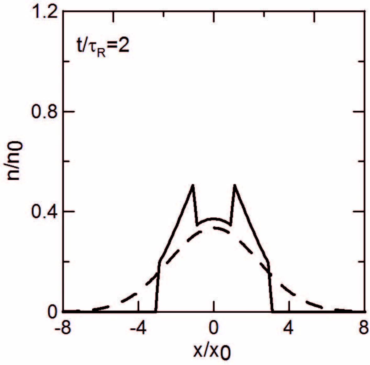
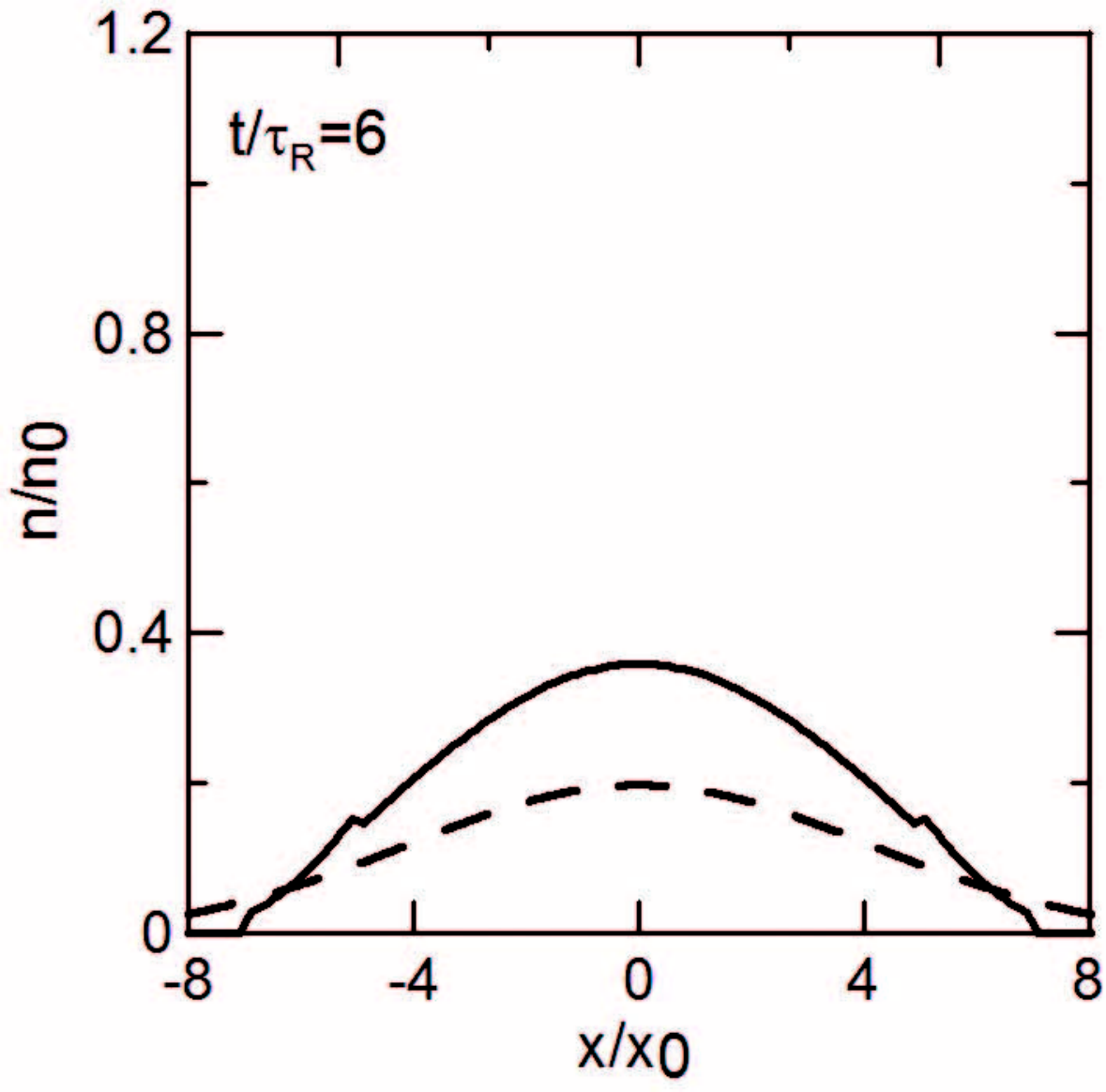
where is the modified Bessel function, and and are initial conditions of the conserved density and corresponding current, respectively. The maximum propagation speed of this equation is characterized by ,
| (10) |
which diverges in the diffusion limit (). In Fig. 2, the time evolutions of the diffusion equation and the telegraph equation are shown by the dashed and solid lines. We use , leading to . The initial denstiy distribution is plotted in the figure of by the dotted line, and we further set . One can see that, because of the memory effect, there exists a non-trivial structure at the boundary of the expanding , reflecting the initial distribution in the telegraph equation, although the diffusion equation always shows the Gaussian forms. Of course, because of the finite propagation speed, the expansion of the telegraph equation is slower than that of the diffusion equation. See also Ref. [2].
In table 1, the comparison of the diffusion equation and the MCV equation is summarized. If the diffusion equation is a coarse-grained dynamics of the underlying microscopic physics, it should be derived from a microscopic theory using systematic coarse-graining. As a matter of fact, as is discussed in textbooks, it is believed that the diffusion equation can be derived with the projection operator method. However, we should note that one non-trivial approximation is used in this derivation. As a matter of fact, it was recently found that, when such non-trivial approximation is not applied, the MCV equation is obtained instead of the diffusion equation [3].
Correspondingly, the microscopic Hamiltonian which describes a diffusion process should have a symmetry associated with the conserved density, and we can derive the corresponding sum rule. The sum rule determines the initial time evolution of the conserved density. The telegraph equation is consistent with this sum rule, although the diffusion equation is not [3, 4].
As is well known in linear irreversible thermodynamics, the positivity of the entropy production is algebraically satisfied when there is a simple linear relation between and . However, this linear relation is not satisfied in the MCV equation. Moreover, when there is no clear separation of time scales, we cannot assume quasi-adiabatic changes of thermodynamical variables, and then heat will play a more fundamental role instead of entropy. Thus the second law for the MCV equation is not trivial. As for the problem of positivity, see Ref. [5].
| diffusion | MCV | |
|---|---|---|
| propagation speed | ||
| microscopic derivation | ? | \tiny⃝ |
| sum rule | \tiny⃝ | |
| 2nd law of thermodynamics | \tiny⃝ | ? |
| positivity | \tiny⃝ | ? |
III modified MCV equation
So far, we have considered currents induced by gradients of . However, when there exists a macroscopic velocity , the total current is given by two contributions,
| (11) |
and the conserved density should satisfy the equation of continuity with instead of itself. In this more general case, the MCV equation is modified [6].
Remember that the conserved density , the velocity and the thermodynamics force are defined by the averaged quantities of particles which are contained inside a small but finite volume , commonly refered to as fluid cell [7]. Thus, Fick’s law should be expressed for quantities per unit cell,
| (12) |
Note that is a function of time because of the deformation induced by the macroscopic flow. In the case of Fick’s law, however, is a common factor and we can finally reproduce the ordinary result (4). On the other hand, Eq. (5) is modified as
| (13) |
Because of the different time dependence of , the deformation of the fluid cell affects the evolution of the current . The dynamics of the fluid cell is determined from a geometrical argument. Now we introduce three vectors to define the volume of the fluid cell, . Because of the macroscopic velocity , any vector is shifted to . Finally we can derive the following equation for the deformation of the fluid cell,
| (14) |
Combining Eqs. (13) and (14), we obtain the modified MCV equation [6],
| (15) |
Interestingly enough, the final result does not depend on the volume of the fluid cell .
The second term on the l.h.s. is a new term which does not exist in the MCV equation, and disappears when there is no macroscopic velocity. In the vanishing limit, this equation still reproduces Fick’s law (4).
The importance of the dynamics of volume elements is discussed also by Brenner [8], where an additional velocity variable is introduced. In our case, however, we do not introduce any additional velocity.
So far, we have discussed the modification of the diffusion equation by introducing a memory effect. There are, however, several different approaches to obtain modified diffusion equations. For example, there are attempts to obtain the MCV equation from the random walk model including memory effect, which is called the persistent random walk. So far, this approach reproduces the MCV equation only for the 1+1 dimensional case [9]. In our work, the memory function has been assumed to have the exponential form. Other possibilities for the memory function are summarized in Ref. [10]. Moreover, as is discussed in Ref. [11], the problem of acausality may be solved by introducing a non-linear effect. van Kampen also discussed modifications of the diffusion equation, associated with the heat conduction of a photon gas [5]. The memory effect for phase separation is discussed in Ref. [12]
IV relativistic fluid dynamics
The problem of the violation of causality becomes more important in deriving relativistic fluid dynamics. In the following, we use the natural unit, where , and the metric .
In the derivation, we first choose gross variables which are necessary to extract the macroscopic motion of many-body systems. If the chosen variables are not enough, the derived fluid dynamics will show unphysical behaviors, such as instability [13, 14] and the divergent transport coefficients [3]. Unfortunately, there is no systematic procedure to collect the complete set of gross variables [15], but normally, conserved densities are chosen. In discussing phase transitions, order parameters are also one of the candidates of gross variables. Here we do not consider phase transitions and conserved charges. Then the gross variables are the energy density and fluid velocity contained in the conserved energy-momentum tensor.
In the idealized case, the the energy-momentum tensor is a function only of and . Then, by applying a Lorentz transformation and using the definition of the energy density and pressure , we obtain . Note that is calculated by the equation of state. Since is conserved, we have
| (16) |
This is the relativistic Euler equation.
However, in general, cannot be expressed only by and . We represent this additional component by another second rank tensor . The most general is, then, given by . Conventionally, is expressed using the trace part and traceless part as 11 1 The heat conduction is neglected, because it finally disappears by using the definition of the fluid velocity.. Finally is expressed as
| (17) |
and and are the bulk viscous pressure and the shear stress tensor, respectively, satisfying the orthogonality condition .
The determination of these viscous terms is our next task. In the traditional Landau-Lifshitz theory [16], these are induced instantaneously by the corresponding thermodynamic force, similarly to the diffusion equation,
| (18) |
where and are the bulk and shear viscosities, respectively. The thermodynamic forces and are defined by
| (19) | |||||
| (20) |
When we use these definitions of the viscous terms, we obtain the relativistic NS equation. Because of the instantaneous production of the viscous terms, this equation contains the propagation with infinite speed, as is shown later.
As was discussed for diffusion processes, the violation of causality is solved by introducing the memory effect previously discussed. Because of the existence of the fluid velocity , the modified MCV equation should be applied. The relativistic representation of the modified MCV equation is
| (21) |
Thus the viscous terms satisfying causality are given by
| (22) | |||||
| (23) |
where and are the relaxation times of and , respectively. Here the projection operator is necessary to satisfy the orthogonality relation. In the following, we call this theory the causal dissipative relativistic (CDR) fluid dynamics.
The second terms on the l.h.s. of Eqs. (22) and (23) comes from the deformation of the fluid cells. As is shown in Figs. 3–8 of Ref. [6], these terms are necessary to implement stable numerical calculations with ultra-relativistic initial conditions.
Here, we simply assume that the thermodynamic forces of the modified MCV equation are the same as those of the relativistic NS equation. However, it may be possible to consider the higher order corrections to the thermodynamic forces, as is discussed in the Burnett equation [17].
V causality and stability of relativistic fluids
When relativistic fluids are described by the relativistic NS equation, the fluid is Newtonian because there is a proportional relation between and . On the other hand, the CDR fluid dynamics describes relativistic non-Newtonian fluids because is determined by solving the differential equation.


Then, are relativistic fluids Newtonian or non-Newtonian ? To answer this question, we investigate the stability of these theories [13, 14]. Let us introduce a perturbation around the hydrostatic equilibrium for the 1+1 dimensional system,
| (24) |
where and the fluid velocity is parameterized with as . Then the linearized CDR fluid dynamics is summarized as
| (25) |
where
| (26) | |||||
where , and is the velocity of sound. In the following calculation, we consider a massless ideal gas, where and . Note that the result of the relativistic NS equation is reproduced by taking .
The dispersion relation is obtained from . When , we have one non-propagating mode and two propagating modes. From the propagating modes, the group velocity is calculated as
| (31) |
One can see that the group velocity diverges in the vanishing limit. That is, the relativistic NS theory contains infinite velocity propagations.
In order to study the stability, the imaginary part of the dispersion relations is shown in Fig. 3. We used and where is the entropy density and is the inverse of temperature. In this parameter set, the group velocity is , which is a causal parameter set because the speed is slower the speed of light. The relativistic NS equation (left panel) has two solutions and the CDR fluid dynamics (right panel) has three solutions. All the imaginary parts are positive and both theories are stable. This result was already known in Ref. [18].


If the theories are consistent with the relativistic kinematics, the nature of stability should not be changed by the Lorentz transform. To see this, we study the stability from a Lorentz boosted frame with a boost velocity of . As is shown in Fig. 4, one of the imaginary parts of the relativistic NS equation (left panel) becomes negative. On the other hand, the imaginary parts of the CDR fluid dynamics (right panel) are always positive. That is, the relativistic NS equation is inconsistent and inadequate as the theory to describe relativistic dynamics.
These results suggest that the violation of causality and instability are correlated. To confirm this, we study the stability of the CDR fluid dynamics with an acausal parameter set, , where the group velocity exceeds the speed of light, . The result is given in Ref. [6]. Again, one of the imaginary part becomes negative in a Lorentz boosted frame, although all the imaginary parts are positive in the rest frame. That is, the violation of causality and instability is intimately related, and it is concluded that relativistic fluids are non-Newtonian. The results are summarized in table 2. So far, we have discussed the bulk viscous pressure. The same result is obtained even for the shear viscous tensor [14].
| RNS | CDR (acausal parameter) | CDR(causal parameter) | |
|---|---|---|---|
| Rest frame | stable | stable | stable |
| Boosted frame | unstable | unstable | stable |
VI Transport coefficients of CDR fluid dynamics
In fluid dynamics, transport coefficients are inputs which should be calculated from the underlying microscopic dynamics. In classical and non-relativistic NS fluids, it is known that the shear viscosity, for example, shows the following density dependence 22 2 So far, the coefficient has not measured experimentally. It will mean that is not a good expansion parameter of [20]. [19],
| (32) |
The first term can be calculated from two different approaches: the Chapman-Enskog expansion of the Boltzmann equation and the Green-Kubo-Nakano (GKN) formula. It is known that the both results are consistent. On the other hand, the higher order coefficients and are not calculated from the Boltzmann equation and we should use the GKN formula 33 3 The Bogoliubov-Choh-Uhlenbeck equation should be used for calculating the higher order terms in the kinetic approach..
However, we cannot use the GKN formula to estimate the transport coefficients of the CDR fluid dynamics, because the GKN formula is derived by assuming the fluid to be Newtonian. Thus we have to derive a new formula to calculate the transport coefficients of the CDR fluid dynamics.
The formula is derived by using the projection operator method [21, 22]. The results are summarized as
| (33) | |||
| (34) |
where denotes operator, and with the equilibrium density matrix . Here and are the shear and bulk viscosities of Newtonian fluids which are calculated using the GKN formula (more exactly, the Zubarev method). One can see that the new transport coefficients are still calculated from the GKN formula with the normalization factors given by the static correlation functions.
The same coefficients can be calculated from the Boltzmann equation with Grad’s moment method [23, 24]. Now we compare the new formula with the Boltzmann equation. For this purpose, we calculate the quantities and , because these are independent of the choice of the collision term of the Boltzmann equation. The behaviors of and are shown on the left and right hand sides of Fig. 5, respectively. The results from the new formula are shown by the solid lines. Note that, as was discussed in Eq. (32), the Boltzmann equation can be consistent with the microscopic formula only in the dilute gas limit. Thus we calculate the ratios in the leading order perturbative approximation.


So far, two different results for the same ratios are known from the Boltzmann equation; one is the well-known result obtained by Israel and Stewart (IS) [23], and the other the result obtained recently by Denicol et al. (DKR) [24] 44 4 The same ambiguity of Grad’s moment method is recently discussed even for non-relativistic cases [17].. The former and latter are plotted by the dotted and dashed lines, respectively. The DKR results predict larger ratios than those of IS, but are still smaller than the results of the microscopic formula.
This difference comes from the effect of quantum fluctuations. In order to incorporate the quantum effect in the Boltzmann equation, the collision term is modified. The ratios are, however, independent of the collision term and hence quantum corrections are not included. Thus, to compare the two results, the effect of quantum fluctuations should be neglected. Then we find that the solid lines agree with the dashed lines [22]. As is shown in Fig. 5, the effect of these fluctuations is quantitatively large and cannot be ignored even in the high temperature limit.
VII Summary
We discussed the infinite propagation speed of the diffusion equation and introduced the Maxwell-Cattaneo-Vernotte (MCV) equation to solve this problem. The drawback and advantage of the diffusion and MCV equations are summarized in table 1. The MCV equation should be modified when there exists a macroscopic flow.
By using this modified MCV equation, we derived a relativistic fluid-dynamical model called the causal dissipative relativistic (CDR) fluid dynamics. On the other hand, another relativistic fluid model was obtained by the relativistic generalization of the Navier-Stokes (NS) theory. To see which theory is more adequate, the stability of the theories was studied with linear analysis. Then we found that the violation of causality and instability are intimately related and the theory becomes unstable if it contains acausal propagations. The relativistic NS theory contains such propagation, and hence is unstable, while the CDR fluid dynamics is causal and stable. In this sense, all relativistic fluids must be non-Newtonian.
Finally, we discussed the calculation of transport coefficients of the CDR fluid dynamics. Because of their non-Newtonian nature, the Green-Kubo-Nakano (GKN) formula is not applicable. The formulae for the CDR fluid dynamics are shown in Eqs. (33) and (34). These formulae are consistent with the results of the Boltzmann equation with Grad’s moment method.
This work was supported by CNPq, FAPERJ and the Helmholtz International Center for FAIR within the framework of the LOEWE program launched by the State of Hesse.
References
- [1] P. M. Morse and H. Feshbach, Methods of Theoretical Physics, (McGraw-Hill Science, 1953)
- [2] J. Masoliver and G. H. Weiss, Eur. J. Phys. 17, 190–196 (1996); J. M. Porrá, J. Masoliver and G. H. Weiss, Phys. Rev. E55, 7771–7774 (1997); M. Abdel Aziz and S. Gavin, Phys. Rev. C70, 034905 (2004).
- [3] T. Koide, Phys. Rev. E 72, 026135-(1)–(10) (2005).
- [4] L. P. Kadanoff and P. C. Martin, Ann.Phys. 24, 419 (1963).
- [5] N. G. van Kampen, Physica 46, 315–332 (1970).
- [6] G. S. Denicol, T. Kodama, T. Koide and Ph. Mota, J. Phys. G36, 035103-(1)–(22) (2009).
- [7] H. D. Weymann, Am. J. Phys. 35, 488–496 (1967); ibid. 37, 232–232 (1969); B. Bertmn and R. A. Guyer, ibid. 37, 231–231 (1969).
- [8] H. Brenner, Internat. J. Eng. Sci 47, 930–958 (2009) and references therein.
- [9] S. Goldstein, Q. J. Mech. Appl. Meth. 4, 129 (1951); J. Masoliver, J. M. Porrá and G. H. Weiss, Physica A182, 593 (1992); ibid. 193, 469 (1993); J. M. Porrá, J. Masoliver and G. H. Weiss Physica. 218, 229 (1995); S. Godoy and L. S. García-Colín, Phys. Rev. E55, 2127 (1997); M. Boguñá, J. M. Porrá and J. Masoliver, emphPhys. Rev. E58, 6992–6997 (1998); J. Dunkel, P. Talker and P. Hänggi, Phys. Rev. D75, 043001-(1)–(8) (2007).
- [10] D. D. Joseph and L. Preziosi, Rev. Mod. Phys. 61, 41–73 (1989); ibid. 62, 375–391 (1990).
- [11] W. L. Kath, Physics D12, 375–381 (1984).
- [12] T. Koide, G. Krein and R. O. Ramos, Phys. Lett. B636, 96–100 (2006).
- [13] G. S. Denicol, T. Kodama, T. Koide and Ph. Mota, J. Phys. G35, 115102-(1)–(20) (2008).
- [14] S. Pu, T. Koide and D. H. Rischke, Phs. Rev. D81, 114039-(1)–(16) (2010).
- [15] K. Kawasaki, Ann. Phys. 61, 1–56 (1970).
- [16] L. D. Landau and E. M. Lifshitz, Fluid Mechanics (Pergamon, New York, 1959).
- [17] L. S. García-Colín, Physica 118A, 341–349 (1983); L. S. García-Colín, R. M. Velasco and F. J. Uribe, Phys. Rep. 465, 149–189 (2008).
- [18] W. A Hiscock and L. Lindblom, Phys. Rev. D35, 3723–3732 (1987); A.L.Garcia-Perciante, L. S. Garía-Colín and A. Sandoval-Villalbazo, Gen. Rel. Grav. 41, 1645–1654 (2009).
- [19] J. R. Dorfman, Physica 106A, 77–101 (1981); M. H. Ernst, arXiv:cond-mat/9707146.
- [20] L. S. García-Colín, private communication.
- [21] T. Koide, Phy. Rev. E75, 060103(R)-(1)–(4) (2007); T. Koide and T. Kodama, Phys. Rev. E78, 051107-(1)–(11) (2008); T. Koide, E. Nakano and T. Kodama, Phys. Rev. Lett. 103, 052301-(1)–(4) (2009).
- [22] G. S. Denicol, X. Huang, T. Koide and D. H. Rischke, arXiv:1003.0780.
- [23] W. Israel and J. M. Stewart, Ann. Phys. (N.Y.) 118, 341–372 (1979).
- [24] G. S. Denicol, T. Koide and D. H. Rischke, arXiv:1004.5013.