Decomposition of Geometric Set Systems and Graphs
Decomposition of Geometric
Set Systems and Graphs
Dissertation
Dömötör Pálvölgyi
Jury:
Prof. J. Pach, thesis director
Prof. F. Eisenbrand, president
Prof. A. Shokrollahi, rapporteur
Prof. G. Rote, rapporteur
Prof. P. Valtr, rapporteur
![[Uncaptioned image]](1009.4641v2/epfllogo.png)
Abstract
We study two decomposition problems in combinatorial geometry. The first part of the thesis deals with the decomposition of multiple coverings of the plane. We say that a planar set is cover-decomposable if there is a constant such that any -fold covering of the plane with its translates is decomposable into two disjoint coverings of the whole plane. Pach conjectured that every convex set is cover-decomposable. We verify his conjecture for polygons. Moreover, if is large enough, depending on and the polygon, we prove that any -fold covering can even be decomposed into coverings. Then we show that the situation is exactly the opposite in three dimensions, for any polyhedron and any we construct an -fold covering of the space that is not decomposable. We also give constructions that show that concave polygons are usually not cover-decomposable. We start the first part with a detailed survey of all results on the cover-decomposability of polygons.
The second part of the thesis investigates another geometric partition problem, related to planar representation of graphs. Wade and Chu defined the slope number of a graph as the smallest number
with the property that has a straight-line drawing with edges
of at most distinct slopes and with no bends.
We examine the slope number of bounded degree graphs. Our main results are that if the maximum degree is at least , then the slope number tends to infinity as the number of vertices grows but every graph with maximum degree at most can be embedded with only five slopes. We also prove that such an embedding exists for the related notion called slope parameter. Finally, we study the planar slope number, defined only for planar graphs as the smallest number with the property that the graph has a straight-line drawing in the plane without any crossings such that the edges are segments of only distinct slopes.
We show that the planar slope number of planar graphs with bounded degree is bounded.
Keywords. Multiple coverings, Decomposability, Sensor networks, Hypergraph coloring, Graph drawing, Slope number, Planar graphs.
Résumé
Nous étudions deux problèmes de décomposition de la géométrie combinatoire. La première partie de cette thèse s’intéresse à la décomposition des recouvrements multiples du plan. On dit qu’un ensemble planaire est recouvrement-décomposable**
*
cover-decomposable s’il existe une constante de telle sorte que tous les -fois recouvrements du plan avec ses translatées sont décomposables en deux recouvrements disjoints du plan tout entier. Pach a conjecturé que tout ensemble convexe est recouvrement-décomposable. Nous vérifions sa conjecture pour les polygones. De plus, si est assez grand, en fonction de et du polygone, nous montrons que tous les -fois recouvrements peuvent être décomposés même en recouvrements. Ensuite, nous montrons qu’en trois dimensions la situation est exactement l’inverse: pour n’importe quel polyèdre et pour tout , nous construisons une -fois recouvrement de l’espace qui n’est pas décomposable. Nous donnons également des constructions qui montrent que les polygones concaves ne sont généralement pas recouvrement-décomposables. Nous commençons la première partie avec une étude détaillée de tous les résultats sur la recouvrement-décomposabilité de polygones.
La deuxième partie de la thèse étudie un autre problème de partition géométrique, lié à la représentation planaire des graphes. Wade et Chu ont défini le
nombre de pente††
†
slope number d’un graphe comme le plus petit nombre avec la propriété que peut être dessiné avec des segments ayant au plus pentes distinctes. Nous examinons le nombre de pente des graphes de degré borné. Nos principaux résultats sont que, si le degré maximum du graphe est d’au moins , alors le nombre de pente tend vers l’infini quand le nombre de sommets croît, mais tout graphe de degré au plus peut être plongé dans le plan avec seulement cinq pentes. Nous montrons aussi qu’un tel plongement existe pour la notion appelé paramètre de pente‡‡
‡
slope parameter. Enfin, nous étudions le nombre de pente planaire§§
§
planar slope number, défini seulement pour les graphes planaires, comme le plus petit nombre avec la propriété que le graphe admet un dessin linéaire dans le plan sans intersections et tel que les segments sont de seulement pentes distinctes.
Nous montrons que le nombre de pente planaire des graphes planaires de degré borné est borné.
Mots-clés. Recouvrements multiples, Décomposabilité, Réseaux de sensors, Coloration des hypergraphes, Dessinage des graphes, Nombre de pente, Graphes planaires.
“I’ll keep it short and sweet. Family, religion, friendship. These are the three demons you must slay if you wish to succeed in business.”
C. Montgomery Burns
I would like to thank all those who in this way or that helped in the creation of the thesis. First of all, of course, my co-authors, Balázs, Géza and Jani, without whom the thesis would consist of at most one chapter (my CV). It would be impossible to enumerate how much the three of them helped, so I have to refrain to one sentence each. Balázs, thank you for buying beer for those unforgettable research sessions at your home, and for writing the first sketch of our proofs that I could rewrite into a paper. Géza, thank you for spending so much of your time with working with me, and for rewriting my always incomprehensible arguments. János, thank you for beguiling me into the unabandonable fields of discrete geometry, for inviting my future-in-the-past wife and for rewriting Géza’s version.
I am also indebted to my supervisor at ELTE, Zoltán Király. Most papers in this thesis were started when I was your student, and although together we usually worked on other topics, you always encouraged me to also pursue this direction. I could not count how many of my conjectures (some of which were related to cover-decomposition) you have disproved. I would also thank all the others from Budapest who helped my combinatorial career, including but not restricted to András, Balázs, Cory, Dani, Gábor, Gyula, Máté, Nathan and Zoli.
I would also like to thank Thomas for letting me copy-paste the tex files of his thesis and for showing me the very important procedure of how to attach the pages together. I am sorry that I replaced your text between with mine. I would like to thank all other members and visitors of the DCG and DISOPT groups for creating such a wonderful extraworkular environment. Thank you Adrian, Andreas, Andrew, Dave, Filip, Fritz, Genna, Jarek, Jocelyne, Judit, Laura, Martin, Nicolai, Paul, Rado, Rom, Saurabh and Scruffy. I wish you all the best and many more happy days in Lausanne!
From the third floor, I would also like to thank Dani for the time we spent together, and for simultaneously translating my abstract to french and correcting the mistakes in the english version. I would also thank here Bernadett, Panos and the anonymous referees of my papers for their valuable comments.
I would like to thank all my jury members, especially Günter and Pavel, for their careful reading and useful comments, most of which I implemented in this corrected version.
Finally, I would like to thank my family for their support. Thank you anya, apa, Déni¶¶
¶
Since I know that you will read this before you leave for the bike tour, I wanted to remind you to buy some chocolate for my birthday. You know, just because we did not meet it does not mean you can skip my present.
Damn, on the other hand, it is kinda hot, so it would melt. Or will you have a cooling box or something like that with you? You know what, just forget about it and get me something after you are back., Eszter, Bence.
But most importantly, I would like to thank my wife, Padmini, who fits to several above mentioned categories. Thank you for leaving me a few seconds each day to work on my research, for reading and spotting so many grammatical mistakes and for all the time we spent together, but maybe the beginning of my thesis is not the best place to discuss this in more detail.
And now for something completely different…
1 Introduction and Organization
Partitions are one of the best studied and most important notions of combinatorial mathematics. The number theoretic partition function , which represents the number of possible partitions of a natural number , was already studied by Euler. Later many mysterious identities about it were proved by Ramanujan and many more are still studied today, including properties of Young-tableaux. In combinatorics, partitions are often called colorings, which is just another more visual way to imagine the decomposition of a set. Coloring the vertices or edges of a graph is probably the problem that fascinated mathematicians more than any other graph theoretical question, from the four-color conjecture to Ramsey theory. The investigation of Property B∥∥
∥
Named after Felix Bernstein who first studied this property. was popularized by Erdős. A set system is said to have Property B if the elements of its ground set can be colored with two colors such that no set is monochromatic, i.e. each set contains both colors. This is strongly connected to the following geometric problem.
Suppose we have a finite number of sensors in a planar region , each monitoring some
part of , called the range of the sensor.
Each sensor has a duration for which it can be active and once
it is turned on, it has to remain active until this duration is over, after
which it will stay inactive. A schedule for the sensors is a starting time for each sensor that determines when it starts to be active.
The goal is to find a schedule to monitor for as long as we can.
For any instance of this problem, define a set system as follows.
The sensors will be the elements of the ground set of and the points of will be the sets.
An element is contained in a set if the respective sensor monitors the respective point.
In the special case when the duration of each sensor is unit of time, we can monitor for units of time if and only if has Property B.
Pach posed the following related problem. Suppose that every point of the plane is covered by many translates of the same planar set. Is it always possible to decompose this covering into two coverings? Thus our goal is to partition/color the covering sets such that every point will be contained in both parts/color classes.
This question is again equivalent to asking whether certain families have Property B.
Pach conjectured that for every convex set there is a constant such that any -fold covering is decomposable into two coverings. Such sets are called cover-decomposable.
The first part of this thesis is centered around this conjecture in the case when the underlying set is a polygon. We show that convex polygons are cover-decomposable. Moreover, if is large enough, depending on and the polygon, we prove that any -fold covering can even be decomposed into coverings. Then we show that the situation is exactly the opposite in three dimensions. For any polyhedron and any , we construct an -fold covering of the space that is not decomposable. We also give constructions that show that concave polygons****
**
A polygon is concave if it is not convex. are not usually cover-decomposable. We start the first part with a detailed survey of all results on the cover-decomposability of polygons.
In the second part we investigate another geometric decomposition problem related to planar representation of graphs. Partitioning the edges of a graph to obtain nice drawings or to show that the graph is complex in some sense was studied under various constraints.
The thickness of a graph
is defined as the smallest number of planar subgraphs it can be decomposed into. It is one of the
several widely known graph parameters that measures how
far is from being planar.
The geometric thickness of , defined as the
smallest number of crossing-free subgraphs of a straight-line
drawing of whose union is , is another similar notion.
In this thesis we investigate a related parameter
introduced by Wade and Chu.
The slope number of a graph is the smallest number
with the property that has a straight-line drawing with edges
of at most distinct slopes and with no bends.
It follows directly from
the definitions that the thickness of any graph is at most as
large as its geometric thickness, which, in turn, cannot exceed
its slope number.
Therefore the slope number is always an upper bound for the other two parameters.
The slope number is also important for the visualization of graphs.
Graphs with slope number two can be embedded in the plane using only vertical and horizontal segments. Generally, the smaller the slope number is, the simpler the visualization becomes.
The second part examines the slope number of bounded degree graphs. Our main results are that if the maximum degree is at least , then the slope number tends to infinity as the number of vertices grow, but every graph with maximum degree at most can be embedded with only five slopes.
The degree case remains a challenging open problem.
We also prove that such an embedding exists for the related notion called slope parameter, which is defined in the second part.
Finally, we study the planar slope number of bounded degree graphs. This parameter is only defined for planar graphs. It is the smallest number with the property that the graph has a straight-line drawing in the plane without any crossings, such that the edges are segments of only distinct slopes. We show that the planar slope number of planar graphs with bounded degree is bounded.
In the third part we summarize the interesting open questions and conjectures about cover-decomposition and the slope number. These are followed by the bibliography and my curriculum vitæ.
Part I Decomposition of Multiple Coverings
2 Introduction and Survey
This section mainly follows our manuscript with János Pach and Géza Tóth, Survey on the Decomposition of Multiple Coverings [PPT10].
Let be a collection of planar sets. We say that is an -fold covering if every point in the plane is contained in at least members of . The biggest such is called the thickness of the covering. A -fold covering is simply called a covering.
Definition. A planar set is said to be cover-decomposable if there exists a (minimal) constant such that every -fold covering of the plane with translates of can be decomposed into two coverings.
We will also refer to the problem of decomposing a covering as the Cover Decomposition problem. Pach [P80] proposed the problem of determining all cover-decomposable sets in 1980 and made the following conjecture.
Conjecture. (Pach) All planar convex sets are cover-decomposable.
This conjecture has been verified for open polygons through a series of papers.
Theorem A. (i) [P86] Every centrally symmetric open convex polygon is cover-decomposable.
(ii) [TT07] Every open triangle is cover-decomposable.
(iii) [PT10] Every open convex polygon is cover-decomposable.
In fact, in [PT10] a slightly stronger result is proved. In particular, it is shown that the union of finitely many copies of the same open convex polygon is also cover-decomposable. See also Section 3 for details. There are several recent negative results as well.
Theorem B. [PTT05] Concave quadrilaterals are not cover-decomposable.
In [PTT05] it was also shown that certain type of concave polygons are not cover-decomposable either. This has been generalized to a much larger class of concave polygons in [P10], see Section 4 for details. One can ask analogous questions in higher dimensions, and in [P10] it is shown that the situation is quite different.
Theorem B’. [P10] Polytopes are not cover-decomposable in the space and in higher dimensions.
For a cover-decomposable set , one can ask for the exact value of . In most of the cases, the best known upper and lower bounds are very far from each other. For example, for any open triangle we have , for the best upper bound see Ács [A10].
Definition. Let be a planar set and integer. If it exists, let denote the smallest number with the property that every -fold covering of the plane with translates of can be decomposed into coverings.
We conjecture that exists for all cover-decomposable , but we cannot prove it in general, see also Question 9.2. In [P86] it is shown that for any centrally symmetric convex open polygon , exists and where is an exponential function of for any fixed . In [TT07] a similar result was shown for open triangles and in [PT10] for open convex polygons. However, all these results were improved to the optimal linear bound in a series of papers.
Theorem C. (i) [PT07] For any centrally symmetric open convex polygon , .
(ii) [A08] For any centrally symmetric open convex polygon , .
(iii) [GV10] For any open convex polygon , .
The problem of determining can be reformulated in a slightly different way: we try to decompose an -fold covering into as many coverings as possible. This problem is closely related to the Sensor Cover problem. Gibson and Varadarajan in [GV10] proved their result in this more general context. See Section 2.3.3 for details.
The goal of this section is to sketch the methods used in the above theorems, and to state the most important open problems. The first paper in this topic was [P86], and its methods were used by all later papers. Therefore, we first concentrate on this paper, and then we turn to the others.
2.1 Basic Tricks
Suppose that we have a -fold covering of the plane with a family of translates of an open polygon . By a standard compactness argument, we can select a subfamily which still forms a -fold covering, and is locally finite. That is, each point is covered finitely many times. Therefore, we will assume without loss of generality that all coverings are locally finite.
2.1.1 Dualization method
In [P86] the results are proved in the dual setting. Suppose we have a collection of translates of . Let be the center of gravity of . The collection is a -fold covering of the plane if and only if every translate of , the reflection of through the origin, contains at least points of the collection .
The collection can be decomposed into two coverings if and only if the set can be colored with two colors, such that every translate of contains a point of each of the colors. Note that the cardinality of can be arbitrary. Using that and are either both cover-decomposable, or none of them is, we have proved the following.
Lemma 2.1.
is cover-decomposable if and only if there is an , such that given any point set , with the property that any translate of contains at least points of , can be colored with two colors such that any translate of contains points of both colors.
Note that the same argument applies if we want to decompose the covering into coverings. All mentioned papers use the same approach, that is, they all investigate the covering problem in the dual setting. Thus, from now on we will also investigate the problem in the dual setting.
2.1.2 Divide et impera – Reduction to wedges
This approach is also from [P86] and it is used in all papers on the topic. Two halflines, both of endpoint , divide the plane into two parts, and , which we call wedges. A closed wedge contains its boundary, an open wedge does not. Point is called the apex of the wedges. The angle of a wedge is the angle between its two boundary halflines, measured inside the wedge.
Let be a polygon of vertices and we have a multiple covering of the plane with translates of . Then, the cover decomposition problem can be reduced to wedges as follows.
Divide the plane into small regions, say, squares, such that each square intersects at most two consecutive sides of any translate of . If a translate of contains sufficiently many points of , then it contains many points of in one of the squares, because every translate can only intersect a bounded number of squares. We color the points of separately in each of the squares such that if a translate of contains sufficiently many of them, then it contains points of both colors. If we focus on the subset of in just one of the squares, then any translate of “looks like” a wedge corresponding to one of the vertices of . That is, if we consider , the wedges corresponding to the vertices of , then any subset of that can be cut off from by a translate of , can also be cut off by a translate of one of . Note that is finite because of the locally finiteness of our original covering.
Lemma 2.2.
is cover-decomposable if there is an , such that any finite point set can be colored with two colors such that any translate of any wedge of that contains at least points of , contains points of both colors.
Again, the same argument can be repeated in the case when we want to decompose a covering into coverings. Thus, from now on, we will be interested in coloring point sets with respect to wedges when proving positive results. But in fact coloring point sets with respect to wedges can also be very useful to prove negative results as is shown by the next lemma.
2.1.3 Totalitarianism
So far our definition only concerned coverings of the whole plane, but we could investigate coverings of any fixed planar point set.
Definition 2.3.
A planar set is said to be totally-cover-decomposable if there exists a (minimal) constant such that every -fold covering of ANY planar point set with translates of can be decomposed into two coverings. Similarly, let denote the smallest number with the property that every -fold covering of ANY planar point set with translates of can be decomposed into coverings.
This notion was only defined in [P10], however, the proofs in earlier papers all work for this stronger version because of Lemma 2.2. Sometimes, when it can lead to confusion, we will call cover-decomposable sets plane-cover-decomposable. By definition, if a set is totally-cover-decomposable, then it is also plane-cover-decomposable. On the other hand, there are sets (maybe even polygons) which are plane-cover-decomposable, but not totally-cover-decomposable. E.g. the disjoint union of a concave quadrilateral and a far enough halfplane is such a set. For these sets the following stronger version of Lemma 2.2 is true.
Lemma 2.4.
The open polygon is totally-cover-decomposable if and only if there is an such that any finite point set can be colored with two colors such that any translate of any wedge of that contains at least points of , contains points of both colors.
Note that if we want to show that a set is not plane-cover-decomposable, then we can first show that it is not totally-cover-decomposable using this lemma for a suitable point set and then adding more points to and using Lemma 2.1. Of course, we have to be careful not to add any points to the translates that show that is not totally-cover-decomposable. This is the path followed in [PTT05] and also in [P10], but there the point set cannot always be extended. This will be discussed in detail in Section 4.
2.2 Boundary Methods
Let be a wedge, and be a point in the plane. A translate of such that its apex is at , is denoted by . More generally, if is convex, then for points , denotes the minimal translate of (for containment) which contains .
Here we sketch the proof of Theorem A (i) from [P86], in the special case when is an axis-parallel square. This square has an upper-left, lower-left, upper-right, and lower-right vertex. To each vertex there is a corresponding wedge, whose apex is at this vertex and whose sides contain the sides of the square incident to this vertex. Denote the corresponding wedges by , , , and , respectively. We refer to these four wedges as -wedges. Let be a finite point set. By Lemma 2.2 it is sufficient to prove the following.
Lemma 2.5.
can be colored with two colors such that any translate of a -wedge which contains at least five points of , contains points of both colors.
It will be very useful to define the boundary of with respect to the wedges of . It is a generalization of the convex hull; a point of is on the convex hull if there is a halfplane which contains on its boundary, but none of the points of in its interior.
Definition 2.6.
The boundary of with respect to a wedge , Two -boundary vertices, and are neighbors if .
It is easy to see that -boundary points have a natural order where two vertices are consecutive if and only if they are neighbors. Observe also that any translate of intersects the -boundary in an interval. Now the boundary of with respect to the four -wedges is the union of the four boundaries.
The - and a -boundary meets at the highest point of (the point of maximum -coordinate, which does not have to be unique, but for simplicity let us suppose it is), the - and a -boundary meets at the rightmost point, the - and a -boundary meets at the lowest point, and the - and a -boundary meets at the leftmost point. See Figure 1. For simplicity, translates of -wedges, , , , , are denoted by , , , , respectively.

Points of which are not boundary vertices, are called interior points. The main difference between the convex hull and the boundary, with respect to , is that in the cyclic enumeration of all boundary vertices obtained by joining the natural orders on the four parts of the boundary together, a vertex could occur twice. These are called singular vertices, the others are called regular vertices. However, it can be shown that no vertex can appear three times in the cyclic enumeration, and all singular vertices have the same type: either all of them belong to and , or all of them belong to and . This also holds for any centrally symmetric convex polygon, singular boundary vertices all belong to the same two opposite boundary pieces.
The most important observation is the following.
Observation 2.7.
If a translate of a -wedge, say, , contains some points of , then it is the union of three subsets: (i) an interval of the boundary which contains at least one point from the -boundary, (ii) an interval of the boundary which contains at least one point from the -boundary, (iii) interior points. Note that (i) is non-empty, while (ii) and (iii) could be empty. Analogous statements hold for the other three wedges, and also for other symmetric polygons.
A first naive attempt for a coloring could be to color all the boundary blue, and the interior red. Clearly, it is possible that there is a wedge that contains lots of boundary vertices and no interior vertices, so this coloring is not always good. Another naive attempt could be to color boundary vertices alternatingly red and blue. There is an obvious parity-problem here, and a problem with the singular vertices. But there is another, more serious problem, that a translate of a wedge could contain just one boundary vertex, and lots of interior vertices. So, we have to say something about the colors of the interior vertices but this leads to further complications. It turns out that a “mixture” of these approaches works.
Definition 2.8.
We call a boundary vertex -rich if there is a translate of a -wedge, such that is the only -boundary vertex in but contains at least points of .†††† †† In [P86] and [PT07] a slightly different definition is used, there is required to be the only vertex from the whole (ant not only from the -) boundary in the translate of . For symmetric polygons both definitions work, but, for example, for triangles only the above given definition can be used.
This definition is used in different proofs with a different constant , but when it leads to no confusion, then we simply write rich instead of -rich. In this proof rich means -rich, thus a boundary vertex is rich if there is a wedge that intersects the -boundary in and contains at least four other points.‡‡‡‡ ‡‡ Note that instead of we could also pick to define rich points in this proof and only the last line would require a little more attention.
Our general coloring rule will be the following.
(1) Rich boundary vertices are blue.
(2) There are no two red neighbors.
(3) Color as many points red as possible, that is, let the set of red points
be maximal under condition (1) and (2).
Note that from (3) we can deduce
(4) Interior points are red.
A coloring that satisfies these conditions is called a proper coloring.
There could be many such proper colorings of the same point set, and for centrally
symmetric
polygons, each of them is good for us.
In [P86] an explicit proper coloring is given.
Now we are ready to finish the argument.
Proof of Lemma 2.5.
Suppose that is colored properly and is a translate of a -wedge, such that it contains at least five points of . We can assume without loss of generality that contains exactly five points of . By Observation 2.7, intersects the -boundary of in an interval.
First we find a blue point in . If the above interval contains just one point then this point is rich as the wedge contains at least five points, and rich points are blue according to (1). If the interval contains at least two points, then one of them should be blue according to (2).
Now we show that there is also a red point in . If contains any interior point, then we are done according to (4). So we can assume by Observation 2.7 that is the union of two intervals, and all points in are blue. Since we have five points, one of them, say, , is not the endpoint of any of the intervals. If it is not rich, then, according to (3), it or one of its neighbors, all contained in , is red. So, should be rich. But then there is a translate of a -wedge, which contains only as a boundary vertex, and contains five points. Using that is centrally symmetric, it can be shown that is a proper subset of , a contradiction, since both contain exactly five points. This concludes the proof of Lemma 2.5.∎
If we only consider wedges with more points, we can guarantee more red points in them.
Lemma 2.9.
In a proper coloring of , any translate of a -wedge which contains at least points of , contains at least one blue point and at least red points.
The proof is very similar to the proof of Lemma 2.5, the difference is that now we color -rich points red and we have to be a little more careful when counting red points, especially because of the possible singular points. Then, we can recolor red points recursively by Lemma 2.9, and we obtain an exponential upper bound on . Analogous statement holds for any centrally symmetric open convex polygon, therefore, we have
Theorem 2.10.
For any symmetric open convex polygon , there is a such that any -fold covering of the plane with translates of can be decomposed into coverings.
2.2.1 Decomposition to parts for symmetric polygons
Here we sketch the proof of Theorem C (i), following the proof of [PT07], which is a modification of the previous proof. We still assume for simplicity that is an axis parallel square. The basic idea is the same as in the previous proof. Let . We will color with colors such that any -wedge that contains at least points contains all colors. We define boundary layers and denote them by , respectively. That is, denote the boundary of by and let . Similarly, for any , once we have , let be the boundary of and let . Boundary layer will be “responsible” for color . Color takes the role of blue from the previous proof, while red points are distributed “uniformly” among the other colors.
Slightly more precisely, a vertex is rich if there is a translate of a -wedge that intersects in at least points, and is the only boundary vertex in it. We color rich vertices of with color , and color first the remaining singular, then the regular points periodically: The main observation is that if a -wedge intersects (for any ) in at least points, then it contains a long interval which contains a point of each color.**** ** This could be improved with a more careful analysis. Otherwise, it has to intersect each of the boundary layers, but then for each , its intersection with contains a rich point of color .
2.2.2 Triangles
The main difficulty with non-symmetric polygons is that Observation 2.7 does not hold here; the intersection with a translate of a -wedge is not the union of two boundary intervals and some interior points. In the case of triangles Tardos and Tóth [TT07] managed to overcome this difficulty, with a particular version of a proper coloring, thus proving Theorem A (ii), we sketch their proof in this section. For other polygons a different approach was necessary, we will see it later.
Suppose that is a triangle with vertices , , . There are three -wedges, , , and . We define the boundary just like before, it has three parts, the -, -, and -boundary, each of them is an interval in the cyclic enumeration of the boundary vertices. Here comes the first difficulty, there could be a singular boundary vertex which appears three times in the cyclic enumeration of boundary vertices, once in each boundary. It is easy to see that there is at most one such vertex, and we can get rid of it by decomposing into at most four subsets, such that in each of them singular boundary points all belong to the same two boundaries, just like in the case of centrally symmetric polygons. For simplicity of the description, assume that has only regular boundary vertices.

Again, we call a boundary vertex rich if there is a translate of a -wedge, such that is the only -boundary vertex in but contains at least five points of .
Our coloring will still be a proper coloring, that is
(1) Rich boundary vertices are blue.
(2) There are no two red neighbors.
(3) Color as many points red as possible, that is, let the set of red points
be maximal under condition (1) and (2).
(4) Interior points are red.
But in this case, we will describe explicitly, how to obtain the set of red points. The coloring will be a kind of greedy algorithm. Consider the linear order on the lines of the plane that are parallel to the side , so that the line through defined smaller than the line . We define the partial order on the points with if the line through is smaller than the line through . We have and . Similarly define the partial order according to the lines parallel to with and , and the partial order according to the lines parallel to with and .
First, color all rich boundary vertices blue. Now take the -boundary vertices of and consider them in increasing order according to . If we get to a point that is not colored, we color it red and we color every neighbor of it blue. These neighbors may have already been colored blue (because they are rich, or because of an earlier red neighbor) but they are not colored red since any neighbor of any red point is immediately colored blue. Continue, until all of the -boundary is colored. Color the - and -boundaries similarly, using the other two partial orders.
Suppose that is a translate of a -wedge, such that it contains at least five points of . We can assume without loss of generality that contains exactly five points of . Assume that is a translate of . The other two cases are exactly the same. To find a blue point, we proceed just like in the previous section, and it works for any proper coloring. We know that intersects the -boundary of in an interval. If this interval contains just one point, then it is rich, so it is blue. It the interval contains at least two points, then one of them should be blue.
Now we show that there is also a red point in . If contains any interior point, then we are done. Therefore, we assume that all five points in are boundary vertices. Since there are five points in , one of them, say, , is not (i) the first or last -boundary vertex in , and (ii) not the -minimal -boundary point in , and (iii) not the -minimal -boundary point in .
Suppose that is rich. Then there is a translate of a -wedge, which contains only as a boundary vertex, and contains five points. It can be shown by some straightforward geometric observations that is a proper subset of , a contradiction, since both contain five points. So, can not be rich. But then why would it be blue? The only reason could be that in the coloring process one of its neighbors on the boundary, , was colored red earlier. But then again, some geometric observations show that , which shows that there is a red point in . This concludes the proof.
The same idea works if we have singular boundary vertices which all belong to, say, to the - and -boundaries. The only difference is that we have to synchronize the coloring processes on the - and -boundaries, so that we get to the common vertices at the same time.
By a slightly more careful argument we obtain
Lemma 2.11.
The points of can be colored with red and blue such that any translate of a -wedge which contains at least of the points, contains a blue point and at least red points.
If we apply Lemma 2.11 recursively, we get an exponential bound on .
Lemma 2.12.
For any open triangle , every -fold covering of the plane with translates of can be decomposed into coverings.
2.3 Path Decomposition and Level Curves
In this chapter we present two generalizations of the boundary method that are used to prove the other positive theorems, Theorem A (iii), C (ii) and C (iii).
2.3.1 Classification of wedges
In order to prove Theorem A (iii), that says all open convex polygons are cover-decomposable, in [PT10] some new ideas were developed. In the previous results we colored a point set with respect to -wedges, for some polygon . In this paper, point sets are colored with respect to an arbitrary set of wedges.
Definition. Suppose that is a collection of wedges. is said to be non-conflicting or simply NC, if there is a constant with the following property. Any finite set of points can be colored with two colors such that any translate of a wedge that contains at least points of , contains points of both colors.*†*† *† Note that if a collection of wedges, is NC, then so is where is the closure or interior of the wedge . This is true because if we perturbate any such that the segment determined by any two points becomes non-parallel to any side of any of the wedges, then the collection of sets of points that can be cut off from by a translate of a wedge from will not decrease.
It turns out that a single wedge is always NC. Then pairs of wedges which are NC are characterized. Finally, it is shown that a set of wedges is NC if and only if each pair is NC. From this characterization it follows directly that for any convex polygon , the set of -wedges is NC.
Lemma 2.13.
A single wedge is NC.
A very important tool in the the proof of Lemma 2.13, and the following lemmas, is the path decomposition which is the generalization of the concept of the boundary. We give the proof of Lemma 2.13 to illustrate this method.
Proof. Let be a finite point set and a wedge. We prove the statement with , that is, can be colored with two colors such that any translate of that contains at least points of , contains a point of both colors. Suppose first that the angle of is at least . Then is the union of two halfplanes, and . Take the translate of (resp. ) that contains exactly two points of , say, and (resp. and ). There might be coincidences between , and , , but still, we can color the set such that and (resp. and ) are of different colors. Now, if a translate of contains three points, it contains either and , or and , and we are done.
Suppose now that the angle of is less than . We show that in this case the NC property holds with . We can assume that the positive -axis is in , this can be achieved by an appropriate rotation. For simplicity, also suppose that no direction determined by two points of is parallel to the sides of as with a suitable perturbation this can be achieved.
For any fixed , let be the translate of
which
(1) contains at most two points of ,
(2) its apex has -coordinate , and
(3) its apex has minimal -coordinate.
It is easy to see that for any , is uniquely defined.
Examine, how changes as runs over the real numbers.
If is very small (smaller than the -coordinate of the points of ),
then contains two points, say and , and one more, , on its boundary.
As we increase , the apex of changes continuously.
How can the set , of the two points in change?
For a certain value of , one of them, say, , moves to the boundary. At
this point we have inside, and two points, , and on the boundary.
If we slightly further increase , then replaces , that is,
and will be in (see Figure 3). As increases to infinity,
the set could change several times, but each time it changes in the above described manner.
Define a directed graph whose vertices are the points of , and there is an edge from to
if replaced during the procedure.
We get two paths, and . The pair is called
the path decomposition of with respect to , of order two (see Figure 4).
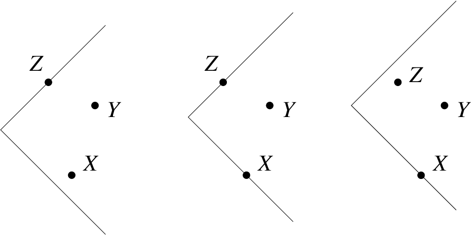
Color the vertices of red, the vertices of blue. Observe that each translate of that contains at least two points, contains at least one vertex of both and . This completes the proof.

We can define the path decomposition of with respect to , of order very similarly. Let be the translate of which (1) contains at most points of , (2) its apex has -coordinate , and (3) its apex has minimal -coordinate. Suppose that for very small, contains the points , and at least one more on its boundary. Just like in the previous description, as we increase , the set changes several times, such that one of its elements is replaced by some other vertex. Define a directed graph on the vertices of such that there is an edge from to if replaced at some point. We get the union of directed paths, , , , , which is called the order path decomposition of with respect to . Note that the order path decomposition is just the -boundary of , so this notion is a generalization of the boundary.*‡*‡ *‡ But in general, is not the boundary for higher order path decompositions! Although the union of the paths contains the boundary, the points of the boundary do not necessarily form a path.
Observation 2.14.
(i) Any translate of contains an interval of each of , , , , and (ii) if a translate of contains points of , then it contains exactly one point of each of , , , .
Now we investigate the case when we have two wedges. We distinguish several cases according to the relative position of the two wedges, and .
Type 1 (Big): One of the wedges has angle at least .
For the other cases, we can assume without loss of generality that contains the positive -axis. Extend the boundary halflines of to lines, they divide the plane into four parts, Upper, Lower, Left, and Right, which latter is itself. See Figure 5.

Type 2 (Halfplane): One side of is in Right and the other one is in Left. That is, the union of the wedges cover a halfplane. See Figure 6.

Type 3 (Contain): Either (i) one side of is in Upper, the other one is in Lower, or (ii) both sides are in Right or (iii) both sides are in Left. See Figure 7.

Type 4. (Hard): One side of is in Left and the other one is in Upper or Lower. This will be the hardest case. See Figure 8.

Type 5. (Special): Either (i) one side of is in Right and the other one is in Upper or Lower, or (ii) both sides are in Upper, or (iii) both sides are in Lower. That is, the union of the wedges is in an open halfplane whose boundary contains the origin, but none of them contain the other. See Figure 9.

It is not hard to see that there are no other possibilities.
Lemma 2.15.
Let be a set of two wedges, of Type 1, 2, 3, or 4. Then is NC.
This lemma is proved in Section 3, for each case separately. It is also shown in [P10] that if is a set of two wedges of Type 5 (Special), then is not NC. For the proof and its consequences see Section 4. In case of several wedges we have
Lemma 2.16.
A set of wedges is NC if and only if any pair is NC.
It is obvious that if two wedges are not NC then can not be NC. Therefore, a set of wedges is NC if and only if none of the pairs is of Type 5 (Special). The proof of Lemma 2.16 can again be found in Section 3. In fact, a somewhat stronger statement is true. At the end of Section 3 it is shown that if is NC, then for any there is an such that any finite point set can be colored with colors such that if a translate of a wedge from contains at least points, then it contains all colors.
To finish the proof of Theorem A (iii), observe that two wedges corresponding to the vertices of a convex polygon cannot be of Type 1 (Big) or of Type 5 (Special). A summary of the whole proof of the theorem can be found at the end of Section 3.
2.3.2 Level curves and decomposition to parts for symmetric polygons
The level curve method was invented by Aloupis et. al. [A08] at the same time and independently from the path decomposition. Again suppose that the angle of is less than and contains the positive -axis. Now define the level curve of depth , , as the collection of the apices of .*§*§ *§ In [A08] they denote this by because they work with closed wedges. Another equivalent way to define is as the boundary of the union of all the translates of containing at most points.
Note that this curve consists of straight line segments that are parallel to the sides of . goes through all the boundary points, this shows that this notion is a generalization of the boundary. If , then is either or and it is only a finite number of times, when the respective translate has a point on both of its sides.
Now with the level curve method, we prove Theorem C (ii), as was done in [A08].
Suppose our symmetric polygon has vertices. We denote the -wedges belonging to them in clockwise order by . All the indices should be considered in this section modulo . We call two wedges and antipodal if modulo , that is, if they are the wedges belonging to two opposite vertices of the polygon. A crucial observation is (already used in [P86]) that any two -wedges that are not antipodal, cover a half-space.
For every side of , take two lines parallel to it that cut off points from each side of . Denote the intersection of the stripes formed by these lines by . Any large enough wedge has to intersect , thus it is enough to care about the wedges whose apex lies in . Now if we consider the level curves , a simple geometric observation shows that only level curves belonging to antipodal wedges may cross inside and some further analysis shows that in fact there can be only one such pair (note the similarity to the singular points in case of symmetric polygons). This means that the regions cut off from by the curves are all disjoint with the possible exception of one pair. Without loss of generality, these are the curves of and .
Another easy observation shows that any translate of that contains at least points, must contain a point from , thus also a translate of whose apex is on the level curve inside , containing points from . Therefore it is enough to care about these wedges, whose apex lies on the respective level curve. It is possible to parametrize these wedges with the circle parameterized by such that is a translate of . A crucial geometric observation is that if , where and , then for all . If , where and , then is contained in two antipodal wedges implying that it is contained in translates of and but in no translates of any other other wedge from . Therefore, every is contained either in an interval of the circle , or in two intervals, one of which is a subinterval of , the other of . The simplest is if we take care of these two types separately, as any big wedge contains a lot of points from one of these groups. The first type forms a circular interval graph, if every point of the circle is covered -fold, then we can decompose this to coverings with a simple greedy algorithm. In the second type, we want to color points with respect to a wedge and its rotation with degrees. The greedy algorithm again gives a good decomposition from an -fold covering into coverings. Putting the numbers together this implies that for any system of wedges derived from a symmetric polygon. This has to be multiplied by a constant depending on the shape of the polygon that comes from Lemma 2.2 to get a bound for the multiple-cover-decomposability function of the polygon.
2.3.3 Decomposition to parts for all polygons
The decomposition to multiple coverings is also motivated by the following problem, called Sensor Cover problem.
Suppose we have a finite number of sensors in a region , each monitoring some part of , which is called the range of the sensor. Each sensor has a duration for which it can be active and once it is turned on, it has to remain active until this duration is over, after which it will stay inactive. The load of a point is the sum of the durations of all ranges that contain it, and the load of the arrangement of sensors is the minimum load of the points of . A schedule for the sensors is a starting time for each sensor that determines when it starts to be active.
The goal is to find a schedule to monitor the given area, , for as long as we can. Clearly, the cover decomposability problem is a special case of the Sensor Cover problem, when the duration of each sensor is the same. Gibson and Varadarajan in [GV10] proved their result in this more general context.
Theorem D. [GV10] For any open convex polygon there is a such that for any instance of the Sensor Cover problem with load where each range is a translate of , there is a polynomial time computable schedule such that every point is monitored for time units.
In the special case where the duration of each sensor is unit of time and is the whole plane, this is equivalent to Theorem C (iii). As the proof is essentially the same, we will only sketch the proof for this special case to avoid changing terminology. In their proof they use the usual dualization and reduction to wedges, because of which it is enough to prove the following theorem (for the special case).
Theorem D’. [GV10] If is a system of -wedges, then there is an depending only on , such that any point set can be colored with colors such that any translate of a wedge from that contains at least points, contains all colors.
Note that any two -wedges are of Type 2 (Halfplane), 4 (Hard) or a special case of 3 (Contain). Their main lemma is the following easy observation.
Lemma 2.17.
For any point set , any wedge , any and any , we can partially color the points of with colors such that any translate of that contains points of and at least points of contains at most colored points but contains all colors. Moreover, if a point is colored, then all points in are colored.
Proof.
In every step take a point from that covers a maximal, yet uncovered interval of *¶*¶ *¶ Here and later, the level curves are always with respect to and not to . until the whole curve is covered, then color these points with one color and repeat. ∎
The trick is that we obtain a partial coloring using this lemma for a carefully chosen subset of , any one of the wedges, , and an (constant depending on to be specified later) such that points remain uncolored in any translate of any wedge from that previously contained at least points. After applying this partial coloring times, we are done.
Before we can specify , we need to define an order on the plane for every line that is parallel to the side of a wedge. (Thus together this gives at most orders for general wedges, for -wedges it would give .) The order is very similar to the one used for triangles in [TT07]. For a wedge and a line parallel to one of its sides, define if the line parallel to through intersects . (So in the special case of -wedges, and are the minimal vertices of according to .) For simplicity, we just refer to these orders as the orders defined by the system .
Now we can define . A point is in if there is a translate of containing exactly points from in which is not among the first points in any of the orders defined by . Now let us apply Lemma 2.17 to this , , and . Note that each translate of whose apex lies on the curve will contain at least points of as .
Claim 2.18.
If contains points from , where , then it contains uncolored points after applying the coloring of Lemma 2.17 to , , and .
Proof.
The proof depends on the type of and . First suppose they are of Type 2 (Halfplane). Take a translate of , containing points of . If it does not intersect the level curve , then we did not color any of its points, we are done. If it intersects this level curve, then the intersection can be only one point, . Moreover, contains all the colored points contained in . Since contains at most colored points, we are done if .
The second case we consider is, if they are of Type 3 (Contain), such that a translate of is (not necessarily properly) contained in (the wedge obtained by reflecting to the origin). Take a translate of , containing points of . If it does not intersect the level curve , then we did not color any of its points, we are done. If there is a for which contains at least points, then we are done as only of these can be colored. Otherwise, for any denote by and the points where the boundary of and meet. So if is one of the two ends of the interval , we have or, respectively, . We also know that for any , the wedge contains at least points of . A continuity argument shows that there is a for which both and contain at least points. If this number is at least , then cannot contain any colored points because of the moreover part of Lemma 2.17. This implies that can contain only the at most colored points of . So for this case we need the additional condition .
Finally, notice that in the remaining cases, can be cut into three parts, , and , such that and have a side parallel to one of the sides of and for each there is a halfplane that contains it with , while is contained in . If contains at least points of , then at least one of these three wedges must contain at least points. If it is , then we are done as in the previous case if . If it is one of the other two wedges, then we arrive to our last case.
Suppose contains at least points of , and there is a triangle such that and are among its three wedges. Without loss of generality, suppose that their parallel side is the horizontal, they are contained in the “upward” halfplane and looks right, left. Again, if does not intersect the level curve , then we did not color any of its points, we are done. If it does, then consider the colored points in in increasing order with respect to the order defined by the non-horizontal side of . If there are at most colored points in , then we are done. Otherwise, denote the colored point according to this order by . Since is colored, there is a for which . If , then must contain all the points that are smaller than in the order, a contradiction, as it can contain at most colored points. If , then we can use the property that . A point was selected to from only if there is a translate of containing exactly points from in which is not among the first points in any of the orders defined by . The apex of this translate of must be on . But then also contains the points smaller than in the order defined by the non-horizontal side of , which are necessarily uncolored, thus we are done. ∎
Therefore we are also done with the proof of the theorem. Note that the bound that we get for grows superexponentially with because apart from , we must also guarantee to make sure that also the translates of contain all colors. We would like to remark that this bound can be made exponential by introducing a more sophisticated notation and demanding a different “” for each wedge in each step (so when there are wedges left, then the “” of should be approximately ).
2.4 Indecomposable Constructions
In this section we survey results about coverings that cannot be decomposed into two coverings. The first such example was given in [MP86], where it was shown that the unit ball is not cover-decomposable. Thus for any there is a covering of with unit balls such that every point is covered by at least balls, but the covering cannot be decomposed into two coverings. Later in [PTT05] several other constructions were given, all based on the geometric realization of the same hypergraph not having Property B*∥*∥ *∥ We say that a hypergraph has Property B if the elements of the ground set can be colored with two colors such that any hyperedge contains both colors.. It was shown by Erdős [E63] that the smallest number of sets of size that do not have Property B is at least , so any indecomposable construction must be exponentially big. With a standard application of the Lovász Local Lemma [EL75] it can also be shown for “nice” geomteric sets that if every point is covered by less than exponentially many translates, then the covering is decomposable.
We start by presenting the construction of [PTT05] using concave quadrilaterals proving Theorem B. Then we briefly preview the results of Section 4.
2.4.1 Concave quadrilaterals
We present the construction in the dual case. We suppose that the vertices of the quadrilateral, , are and in this order, the obtuse angle being at . This implies that and are of Type 5 (Special), moreover, they belong to an even more special subclass: When we translate the wedges such that their apices are in the origin, then they are disjoint and there is an open halfplane that contains both of their closures (see the two right examples in Figure 9). For simplicity, let us suppose that is a very thin wedge that contains a horizontal segment and is a very thin wedge that contains a vertical segment, the construction would work for any other two wedges that are derived from a concave quadrilateral.
First we give a finite set of points and a finite number of translates that show that is not totally-cover-decomposable. Then we show how this construction is extendable to give a covering of the whole plane. The construction is based on a construction using translates of the wedges and . We will use these wedges to realize the following -uniform hypergraph, . The vertices of the hypergraph are sequences of length less than consisting of the numbers from through : . There are two kinds of hyperedges. The first kind contains sequences of length whose restriction to their first members is the same. The second kind consists of a length sequence and all its possible restrictions. So has roughly vertices and edges.

The hyperedges of the first kind are realized by translates of , the second kind by translates of . The vertices of the hypergraph are all very close to a vertical line. Also, vertices that belong to a hyperedge of the first kind are all on a horizontal line, for each edge on a different one (see Figure 10). It is easy to see that this is indeed a geometric realization of , so the points cannot be colored with two colors such that every translate of and of size contains both colors.

Now we need to extend the corresponding covering to the whole plane. Before we do, notice that it can be achieved that the centers of all translates of used in the construction lie on the same line. After going back from the dual to the primal, this means that we have a set of points, , on a line, , and an indecomposable, -fold covering of them with translates of . Add all translates of to our covering that are disjoint from (see Figure 11). It is clear that the resulting covering remains indecomposable. Moreover, now every point not in will be covered infinitely many times****** *** The construction can of course be modified to get a locally finite covering using a standard compactness argument., because cannot have two sides that are parallel to , so we can “go in” between any two points of . Note that this statement is not necessarily true for arbitrary concave polygons, this is why the construction of [P10] is not always extendable this way.
2.4.2 General concave polygons and polyhedra
The construction for concave polygons differs from the quadrangular case because it is no longer true that any pair of Type 5 (Special) wedges have the property that they can be translated such that their apices are in the origin and they are disjoint (see the two left examples in Figure 9). Because of this a different hypergraph (also not having Property B) is realized. This construction has less points (about ) and is more general as it can be realized by any pair of Type 5 (Special) wedges. The details can be found in Section 4.
However, this construction is not always extendable to give an indecomposable covering of the whole plane. Different notions of cover-decomposability and their connections are also studied in Section 4. Finally, as a corollary of the construction, it is also shown at the end of Section 4 that polyhedra (both convex and concave) are not cover-decomposable. This construction is extandable, thus we obtain that polyhedra are not space-cover-decomposable.
3 Decomposition of Coverings by Convex Polygons
This section is based on our paper with Géza Tóth, Convex polygons are cover-decomposable [PT10].
Our main result is the strongest statement, (iii), of Theorem A, which claims
Theorem A. Every open convex polygon is cover-decomposable.
We start by recalling some old definitions and making some new ones. Then we establish the earlier unproved Lemma 2.15 and 2.16, and finally, we summarize the proof of Theorem A.
3.1 Preparation
Now let be a wedge, and be a point in the plane. A translate of such that its apex is at , is denoted by . More generally, for points , denotes the minimal translate of (for containment) whose closure contains . The set of all translates of is denoted by and the set of those translates that contain exactly points from a point set is denoted by . The reflection of about the origin is denoted by .
We can assume without loss of generality that the positive -axis is in , and that no two points from our point set, , have the same -coordinate. Both of these can be achieved by an appropriate rotation. We say that if the -coordinate of is smaller than the -coordinate of . This ordering is called the -ordering. A subset of is an interval of if
The boundary of with respect to , Note that a translate of always intersects the boundary in an interval. For each the shadow of is Observe that
Now we give another proof using these notions for Lemma 2.13 that claims that any single wedge, , is NC. In fact, we show that if the angle of is less than , then the points of can be colored with two colors such that any wedge that has at least two points contains both colors (so the NC property holds with ).
Proof. Color the points of the boundary alternating, according to the order . For every boundary point , color every point in the shadow of to the other color than . Color the rest of the points arbitrarily. Any translate of that contains at least two points, contains one or two boundary points. If it contains one boundary point, then the other point is in its shadow, so they have different colors. If it contains two boundary points, then they are consecutive points according to the -order, so they have different colors again. .
3.2 NC wedges - Proof of Lemma 2.15 and 2.16
Now we can turn to the case when we have translates of two or more wedges at the same time. Remember that any pair of wedges belong to a Type determined by their relative position. The different types are classified in Section 2.3.1 and are depicted in Figures 6, 7, 8, 9. It is shown in [P10] that if is a set of two wedges of Type 5 (Special), then is not NC. In a series of lemmas we show that all other pairs are NC, thus proving Lemma 2.15.
Lemma 3.1.
Let be a set of two wedges, of Type 3 (Contain). Then is NC.
Note that this proof could be made slightly simpler with an argument similar to the one used in the proof of Lemma 2.17, here we reproduce the original proof.
Proof. We can assume that or and contains the positive -axis, just like on the two right diagrams of Figure 12. Let be the path decomposition of with respect to , of order .
Observe that any translate of intersects any in an interval of it. Indeed, if , then , which is a subset of . See Figure 13.

We show that we can color the points of with red and blue such that any translate of which contains at least 4 points, and any translate of which contains at least 14 points, contains points of both colors. Consider , the path decomposition of with respect to , of order . We color and such that every contains a blue point of them, and every contains points of both colors. Similarly, we color and such that every contains a red point of them, and every contains points of both colors. Finally, we color the rest of the points such that every contains points of both colors.
Recall that for any , . For any , , if there is a with and , then we say that and are friends. If (resp. ) has only one friend (resp. ), then we call it a fan (of , resp. of ). If or has at least one fan, then we say that it is a star. Those points that are neither fans, nor stars are called regular.
For an example, see Figure 4. On the left figure, is a star, its fans are and , the other points are regular. On the right, is a star, its fan is , the other points are regular.
Suppose first that all points of and are regular. Color every third point of , red and the others blue. In , color the friends of the red points blue, and color the rest of the points of (every third) red. For any , and are friends, therefore, at least one of them is blue. On the other hand, any contains three consecutive points of or , and they have both colors.
Suppose now that not all the points of and are regular. Color all stars blue. The first and last friend of a star, in the -ordering, is either a star or a regular vertex, the others are fans. Color the friends of each star alternatingly, according to the -ordering, starting with blue, except the last two friends; color the last one blue, the previous one red. The so far uncolored regular points of and form pairs of intervals. We color each such pair of interval the same way as we did in the all-regular case, coloring the first point of each pair of intervals red. See Figure 14.
Clearly, if then it contains at least one blue point of . If , then it contains four consecutive points of or , say, , in . If and is a star, then must contain all fans of as well. Indeed, the fans of are in , and by our earlier observations, this is in . So, if either or is a star, then contains a red point, since every star has a red fan. Since the star itself is blue, we are done in this case. If contains three consecutive regular vertices then we are done again, by the coloring rule for the regular intervals. So we are left with the case when and are stars, and are regular. But in this case also contains the common friend of and in , which is also a regular vertex. By the coloring rule for the regular intervals, one of , and is red, the other two are blue, so we are done.
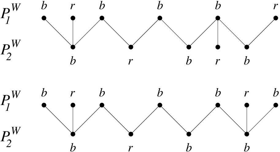
For we use the same coloring rule as for but we switch the roles of the colors. So any contains at least one red point of and any contains both colors.
Finally, we have to color the rest of the points such that every contains points of both colors. This can be achieved by the first proof of Lemma 2.13.
Now any contains at least one blue and at least one red point. If , then either it contains at least two points of , or at least seven points of , or at least seven points of , and in all cases it contains points of both colors. This completes the proof of Lemma 3.1.
Definition 3.2.
Suppose that is a pair of wedges. is said to be asymmetric non-conflicting or simply ANC, if there is a constant with the following property. Any finite set of points can be colored with red and blue such that any translate of that contains at least points of , contains a red point, and any translate of that contains at least points of , contains a blue point.
The next technical result allows us to simplify all following proofs.
Lemma 3.3.
If a pair of wedges is not of Type 5 (Special), and ANC, then it is also NC.
Proof. We can assume without loss of generality that contains the positive -axis, and contains either the positive or the negative -axis. Suppose that is ANC, let arbitrary, and let be a set of points. First we color . Let be a wedge that also contains the positive -axis, but has a very small angle. Then translates of and translates of both intersect in its intervals. Clearly, the pair is of Type 3 (Contain), therefore, by Lemma 3.1, we can color such that any translate of , and any translate of , contains both colors. But then any translate of , contains both colors as well.
Now we have to color . We divide it into three parts as follows.
Any translate that intersects in at least one point, must contain at least one blue point, from , so we only have to make sure that it contains a red point too. Similarly, any that intersects in at least one point, must contain a red point, and any that intersects must contain points of both colors.
Thus, we can simply color such that any contains both colors, which can be done by Lemma 2.13.
With , and with , respectively, we proceed exactly the same way as we did with itself, but now we change the roles of and . We get the (still uncolored) subsets , , , , , with the following properties.
- •
Any translate or , that intersects (resp. ) in at least one point, must contain at least one blue (resp. red) point.
- •
Any translate that intersects (resp. ) contains a blue (resp. red) point, and any translate that intersects (resp. ) contains a red (resp. blue) point.
- •
Any translate that intersects (resp. ) contains a blue (resp. red) point, and any translate that intersects (resp. ) contains points of both colors.
Color all points of and red, color all points of and blue. Finally, color using the ANC property of the pair , and similarly, color also using the ANC property, but the roles of red and blue switched. Now it is easy to check that in this coloring any translate of or that contains sufficiently many points of , contains a point of both colors.
Remark 3.4.
In [P10] it has been proved that if is a Special pair, then is not ANC. So, the following statement holds as well.
Lemma 3.3’. If a pair of wedges is ANC, then it is also NC.
Lemma 3.5.
Let be a set of two wedges, of Type 1 (Big). Then is NC.
Proof. By Lemma 3.3, it is enough to show that is ANC. Let be the wedge whose angle is at least . Then is the union of two halfplanes, say, and . Translate both halfplanes such that they contain exactly one point of , denote them by and , respectively. Note that may coincide with . Color and red, and all the other points blue. Then any translate of that contains at least one point, contains a red point, and any translate of that contains at least three points, contains a blue point.
Lemma 3.6.
Let be a set of two wedges, of Type 2 (Halfplane). Then is NC.
Proof. Again, it is enough to show that they are ANC. Since is of Type 2 (Halfplane), and have at most one point in common. If and are disjoint, then color blue, red, and the other points arbitrarily. Then any nonempty translate of (resp. ) contains a blue (resp. red) point.
Otherwise, let be their common point. Let , and consider its -boundary, , and -boundary, . Clearly, each point in belongs to , and each point in belongs to .
If and are disjoint, then color blue, and the other points red. Then any nonempty translate of contains a blue point. Suppose that we have a translate of with two points, both blue. Then it should contain , and a point of . But this contradicts our assumption that and are disjoint. So, any translate of which contains at least two points of , contains a red point.
If and are not disjoint, then they have one point in common, let be their common point. If belongs to , then color blue, and the other points red. Then, by the same argument as before, any nonempty translate of contains a blue point, and any translate of which contains at least two points of , contains a red point. Finally, if belongs to , then we proceed analogously, but the roles of and , and the colors, are switched.
Lemma 3.7.
Let be a set of two wedges, of Type 4 (Hard). Then is NC.
Proof. As usual, we only prove that is ANC. Assume that contains the positive -axis. Just like in the definition of the different types, extend the boundary halflines of to lines, they divide the plane into four parts, Upper, Lower, Left, and Right, latter of which is itself. We can assume without loss of generality that contains the negative -axis, one side of is in Upper, and one side is in Left, just like on the left of Figure 17.
Observe that if a translate of and a translate of intersect each other, then one of them contains the apex of the other one.
Claim 3.8.
For any point set and , either or .
Proof. Suppose on the contrary that and . Then and , so and intersect each other, therefore, one of them contains the other one’s apex, say, . But this is a contradiction, since is a boundary point of .
Return to the proof of Lemma 3.7. Color red, and blue, the interior points arbitrarily. Now consider the points of . For any , if , then color it red, if , then color it blue. For each of the remaining points we have . Color each of these points such that they have the opposite color than the the previous point of , in the -ordering.
To prove that this coloring is good, let , . If it intersects , we are done. So assume that . Let . If is red, then by the coloring rule, . But then is also a -boundary point, so we have . Again we can assume that is red, so . Suppose that . Since , and are consecutive points of . Now it is not hard to see that . Therefore, by the coloring rule, and have different colors. For the translates of the argument is analogous, with the colors switched.
Now we turn to the case when we have more than two wedges.
Lemma 3.9.
For any integers, there is a number with the following property.
Let be a set of wedges, such that any pair is NC, and let be a set of points. Then can be decomposed into parts, , such that for , for any translate of , if then .
Proof. The existence of is equivalent to the property that the corresponding two wedges are ANC. Now we show that exists for every . Let and be two wedges that form a NC pair. Let be the path decomposition of of order , with respect to . For , let
For each , take the -path decomposition, , and for each , let
For every , color , such that any translate of (resp. ) that intersects it in at least points, contains at least one red (resp. blue) point of it. This is possible, since the pair is ANC.
Consider a translate of that contains at least points of . For every , intersects in points, so there is a such that it intersects in at least points. Therefore, contains at least one red point of , so at least red points of .
Consider now a translate of that contains at least points of . There is an such that intersects in at least points. Therefore, it intersects each of , in at least one point, so for , intersects in at least points. Consequently, it contains at least one blue point of each , so at least blue points of .
Now let fixed and suppose that exists for every . Let be our set of wedges, such that any pair of them is NC. Let . Partition our point set into such that for , for any translate of , if then . For each , partition into two parts, and , such that for any translate of , if then , and for any translate of , if then . Finally, for , let and let . For , any translate of , if then , so ,
And for any translate of , if , then for some , , therefore, , so . This concludes the proof of Lemma 3.9.
Remark 3.10.
As a corollary, we have can now prove Lemma 2.16.
Lemma 2.16. A set of wedges is NC if and only if any pair is NC.
Proof. Clearly, if some pair is not NC, then the whole set is not NC either. Suppose that every pair is NC. Decompose into parts with the property that for , for any translate of , if then . Then, by Lemma 2.13, each can be colored with red and blue such that if then contains points of both colors. So this coloring of has the property that for , for any translate of , if then it contains points of both colors.
3.3 Summary of Proof of Theorem A
Although we have already established Theorem A, we find it useful to give another summary of the complete proof.
Suppose that is an open convex polygon of vertices and is a collection of translates of which forms an -fold covering of the plane. We will set the value of later. Let be the minimum distance between any vertex and non-adjacent side of . Take a square grid of basic distance . Obviously, any translate of intersects at most basic squares. For each (closed) basic square , using its compactness, we can find a finite subcollection of the translates such that they still form an -fold covering of . Take the union of all these subcollections. We have a locally finite -fold covering of the plane. That is, every compact set is intersected by finitely many of the translates. It is sufficient to decompose this covering. For simplicity, use the same notation for this subcollection.
We formulate and solve the problem in its dual form. Let be the center of gravity of . Since is an -fold covering of the plane, every translate of , the reflection of through the origin, contains at least points of the locally finite set .
The collection can be decomposed into two coverings if and only if the set can be colored with two colors, such that every translate of contains a point of both colors.
Let be the set of wedges that correspond to the vertices of . By the convexity of , no pair is of Type 5 (Special), therefore, by the previous Lemmas, each pair is NC. Consequently, by Lemma 2.16, is NC as well. So there is an with the following property.
* Any set of points can be colored with two colors such that any translate of that contains at least points of , contains points of both colors.
Choose such that , and color the points of in each basic square separately, with property *.
Since any translate of intersects at most basic squares of the grid , contains at least points of in the same basic square . By the choice of the grid , contains at most one vertex of , hence , where is a translate of some . So, by property *, contains points of of both colors. This concludes the proof of Theorem A.
3.4 Concluding Remarks
Throughout this section we made no attempt to optimize the constants. However, it may be an interesting problem to determine (asymptotically) the smallest in the proof of Theorem A.
Another interesting question is to decide whether this constant depends only on the number of vertices of the polygon, or on the shape as well. In particular, we cannot verify the following.
Conjecture 3.11.
There is a constant such that any -fold covering of the plane with translates of a convex quadrilateral can be decomposed into two coverings.
With a slight modification of our proof of Theorem A, we get the following more general result about decomposition to coverings.
Theorem A’. For any open convex polygon (or concave polygon without Type 5 (special) wedges), , and any , there exists a (smallest) number , such that any -fold covering of the plane with translates of can be decomposed into coverings.
Our proof gives , where is the constant from the proof of Theorem A and is the number of vertices of . The best known lower bound on is [PT07]. Recently Gibson and Varadarajan [GV10] proved Theorem C (iii), which is a linear upper bound for all convex polygons. However, their proof does not work for any cover-decomposable polygon, because they handle only one case of Type 3 (Contain). For a summary of their result see the end of Section 2. We conjecture that a linear upper bound also holds for cover-decomposable concave polygons.
Conjecture 3.12.
For any cover-decomposable polygon , .
For more related conjectures see Section 9.
Our proofs use the assumption that the covering is locally finite, and for open polygons we could find a locally finite subcollection which is still a -fold covering. Still, we strongly believe that Theorem A holds for closed convex polygons as well.
4 Indecomposable Coverings by Concave Polygons
This section is based on my paper, Indecomposable coverings with concave polygons [P10].
The main goal of this section is to prove results about non-cover-decomposable polygons. To understand some of the results, we need to recall the notions introduced in Section 2.1.3.
Definition 2.3. A planar set is said to be totally-cover-decomposable if there exists a (minimal) constant such that every -fold covering of ANY planar point set with translates of can be decomposed into two coverings. Similarly, let denote the smallest number with the property that every -fold covering of ANY planar point set with translates of can be decomposed into coverings.
When we want to emphasize the difference from the original definition, we will call the cover-decomposable sets plane-cover-decomposable. By definition, if a set is totally-cover-decomposable, then it is also plane-cover-decomposable. On the other hand, we cannot rule out the possibility that there are sets, or even polygons, which are plane-cover-decomposable, but not totally-cover-decomposable.
The results of Theorem A all remain true if we write totally-cover-decomposable instead of cover-decomposable and similarly, in Theorem C we can replace with . In fact in the proofs of these theorems, these more general claims are proved. The proof of Theorem B establishes first that concave quadrilaterals are not totally-cover-decomposable and then extends the covering, proving that they are also not plane-cover-decomposable. The main result of this section is a generalization of Theorem B. We show that almost all (open or closed) concave polygons are not totally-cover-decomposable and prove that most of them are also not plane-cover-decomposable. We need the “almost” because Theorem A’ implies that any concave polygon without Type 5 (Special) wedges is totally-cover-decomposable.
Our main result is the following
Theorem E. If a polygon has a pair of Type 5 (Special) wedges, then it is not totally-cover-decomposable.
Together with the previous theorem, this gives a complete characterization of totally-cover-decomposable open polygons; an open polygon is totally-cover-decomposable if and only if it does not have a Special pair of wedges.
We show that every concave polygon with no parallel sides has a pair of Special wedges, therefore we have
Theorem E’. If a concave polygon has no parallel sides, then it is not totally-cover-decomposable.
The proof of these theorems can be found in Section 4.1.
The problem of deciding plane-cover-decomposability for concave polygons is still open. However, in Section 4.2, we prove that a large class of concave polygons are not plane-cover-decomposable. We also show that any “interesting” covering of the plane uses only countably many translates. (However, we do not consider here the problem when we want to decompose into infinitely many coverings; the interested reader is referred to the paper of Elekes, Mátrai and Soukup [EMS10].)
Finally, in Section 4.3, we investigate the problem in three or more dimensions. The notion of totally-cover-decomposability extends naturally and we can also introduce space-cover-decomposability. Previously, the following result was known.
Theorem F. Mani-Levitska, Pach [MP86] The unit ball is not space-cover-decomposable.
Using our construction, we establish the first theorem for polytopes which shows that the higher dimensional case is quite different from the two dimensional one.
Theorem B’. Polytopes are not cover-decomposable in the space and in higher dimensions.
4.1 The Construction - Proof of Theorems E and E’
In this section, for any and any polygon that has a Special pair of wedges, we present a (finite) point set and an indecomposable -fold covering of it by (a finite number of) the translates of the polygon. We formulate (and solve) the problem in its dual form, like we did before. Here we recall how the dualization goes. Fix , the center of gravity of as our origin in the plane. For the planar set and a point in the plane we use to denote the translate of by the vector . Let be the reflection through of . For any point , if and only if . To see this, apply a reflection through the midpoint of the segment . This switches and , and also switches and .
Consider any collection of translates of and a point set . The collection covers at least times if and only if contains at least elements of the set . Therefore a -fold covering of transforms into a point set such that for every the set contains at least points of . The required decomposition of exists if and only if the set can be colored with two colors such that every translate that contains at least elements of contains at least one element of each color. Thus constructing a finite system of translates of and a point set where this latter property fails is equivalent to constructing an indecomposable covering using the translates of .
If has a Special pair of wedges, then so does . We will use the following theorem to prove Theorem E.
Theorem 4.1.
For any pair of Special wedges, and , and for every , there is a point set of cardinality , such that for every coloring of with red and blue, either there is a translate of containing red points and no blue points, or there is a translate of containing blue points and no red points.
Proof.
Without loss of generality, suppose that the wedges are contained in the right halfplane.
For the statement is trivial, just take points such that any one is contained alone in a translate of . Similarly points will do for . Let us suppose that we already have a counterexample for all and let us denote these by . The construction for and is the following.
Place a point in the plane and a suitable small scaled down copy of left from such that any translate of with its apex in the neighborhood of contains , but none of the translates of with its apex in the neighborhood of does. Similarly place such that any translate of with its apex in the neighborhood of contains , but none of the translates of with its apex in the neighborhood of does. (See Figure 19.)


If is colored red, then
– either the part already contains a translate of that contains reds and no blues, and it contains as well, which gives together red points
– or the part contains a translate of that contains blues and no reds and it does not contain .
The same reasoning works for the case when is colored blue.
Now we can calculate the number of points in . For and for we know that and , while the induction gives . From this we have ∎
It is easy to see that if we use this theorem for a pair of Special wedges of and , then for every coloring of (a possibly scaled down copy of) the above point set with two colors there is a translate of that contains at least points, but contains only one of the colors. This is because “ can locally behave like any of its wedges”. Therefore this construction completes the proof of Theorem E.
Remark 4.2.
Note that we can even give a finite collection of translates of and whose apices all lie on the same line such that one of them will satisfy the conclusion of the theorem. Moreover, this line can be any line that can touch a translate of each wedge in only its apex.
Remark 4.3.
We note that for the cardinality of the point set is approximately , this significantly improves the previously known construction of Pach, Tardos and Tóth [PTT05] which used approximately points and worked only for quadrilaterals, and in general, for “even more Special” pairs of wedges (the ones on the right side of Figure 18). It can be proved that this exponential bound is close to being optimal. Suppose that we have points and Since there are two kinds of wedges, there are at most essentially different translates that contain points. There are different colorings of the point set and each translate that contains points is monochromatic for of the colorings. Therefore, there are at most bad colorings, so there is a coloring with no monochromatic translates.
Theorem E’ follows directly from the next result.
Lemma 4.4.
Every concave polygon that has no parallel sides, has a Special pair of wedges.
Proof.
Assume that the statement does not hold for a polygon . There is a touching line to such that the intersection of and contains no segments and contains at least two vertices, and . (Here we use that has no parallel sides.) Denote the wedges at by . Is the pair Special? They clearly fulfill the property (i), the only problem that can arise is that the translate of one of the wedges contains the other wedge. This means, without loss of generality, that the angle at contains the angle at . Now let us take the two touching lines to that are parallel to the sides of . It is impossible that both of these lines touch , because then the touching line would touch only as well. Take a vertex from the touching line (or from one of these two lines) that does not touch . (See Figure 20.) This cannot be because then the polygon would have two parallel sides. Is the pair Special? They are contained in a halfplane (the one determined by the touching line). This means, again, that the angle at contains the angle at . Now we can continue the reasoning with the touching lines to parallel to the sides of , if they would both touch , then the touching line would touch only . This way we obtain the new vertices what contradicts the fact the can have only a finite number of vertices. ∎

4.2 Versions of Cover-decomposability
Here we consider different variants of cover-decomposability and prove relations between them.
4.2.1 Number of sets: Finite, infinite or more
We say that a set is finite/countable-cover-decomposable, if there exists a such that every -fold covering of any point set by a finite/countable number of its translates is decomposable. So by definition we have: totally-cover-decomposable countable-cover-decomposable finite-cover-decomposable. But which of these implications can be reversed? We will prove that the first can be for “nice” sets.
It is well-known that the plane is hereditary Lindelöf, i.e. if a point set is covered by open sets, then countably many of these sets also cover the point set. It is easy to see that the same holds for -fold coverings as well. This observation implies the following lemma.
Lemma 4.5.
An open set is totally-cover-decomposable if and only if it is countable-cover-decomposable.
The same holds for “nice” closed sets, such as polygons or discs. We say that a closed set is nice if there is a and a set of countably many closed halfdiscs such that if different translates of cover a point , then their union covers a halfdisc from centered at (meaning that is halving the straight side of the halfdisc) and the union of their interiors covers the interior of the halfdisc. For a polygon, can be the number of its vertices plus one, can be the set of halfdiscs whose side is parallel to a side of the polygon and has rational length. For a disc, can be and can be the set of halfdiscs whose side has a rational slope and a rational length. In fact every convex set is nice.
Claim 4.6.
Every closed convex set is nice.
Proof.
Some parts of the boundary of the convex set might be segments, we call these sides. Trivially, every convex set can have only countably many sides. Choose and let the set of halfdiscs be the ones whose side is either parallel to a side of or its slope is rational and has rational length. Assume that different translates of cover a point . Shifting these translates back to , denote the points that covered by . If any of these points is not on the boundary of , we are done. The pentagon has two neighboring angles the sum of whose degrees is strictly bigger than , without loss of generality, and . If is also the side of , then the translates cover a halfdisc whose side is parallel to , else they cover one whose side has a rational slope. ∎
Taking a rectangle verifies that is optimal in the previous proof.
Lemma 4.7.
A nice set is totally-cover-decomposable if and only if it is countable-cover-decomposable.
Proof.
We have to show that if we have an infinite covering of some point set by the translates of our nice, countable-cover-decomposable set , then we can suitably color the points of . Denote by the points that are covered by copies of the same translate of the nice set . Color one of these red, the other blue. Now we only have to deal with and we can suppose that there is only one copy of each translate. Now instead of coloring these translates, we rather show that we can choose countably many of them such that they still cover every point of many times. Using after this that the set is countable-cover-decomposable finishes the proof. So now we show that if there is a set of translates of that cover every point of at least times, then we can choose countably many of these translates that cover every point of at least times. It is easy to see that it is enough if we show this for (since we can repeat this procedure times).
Denote the points that are contained in the interior of a translate by . Because of the hereditary Lindelöf property, countably many translates cover . If a point is covered times, then because of the nice property of , a halfdisc from centered at is covered by these translates. We say that this (one of these) halfdisc(s) belongs to . Take a partition of into countably many sets such that the halfdisc belongs to the points of . Now it is enough to show that can be covered by countably many translates. Denote the halfdisc belonging to the points of by . Using the hereditary Lindelöf property for and open discs (not halfdiscs!) with the radius of centered at the points of , we obtain a countable covering of . Now replacing the open discs with closed halfdiscs still gives a covering of because otherwise we would have such that is in the interior of , but interior of is covered by the interiors of translates of , which would imply , contradiction. Finally we can replace each of the halfdiscs belonging to the points of by translates of , we are done. ∎
Unfortunately, we did not manage to establish any connection among the finite- and the countable-cover-decomposability. We conjecture that they are equivalent for nice sets (with a possible slight modification of the definition of nice). If one manages to find such a statement, then it would imply that considering cover-decomposability, it does not matter whether the investigated geometric set is open or closed, as long as it is nice. For example, it is unknown whether closed triangles are cover-decomposable or not. We strongly believe that they are.
4.2.2 Covering the whole plane
Remember that by definition if a set is totally-cover-decomposable, then it is also plane-cover-decomposable. However, the other direction is not always true. For example take the lower halfplane and “attach” to its top a pair of Special wedges (see Figure 21). Then the counterexample using the Special wedges works for a special point set, thus this set is not totally-cover-decomposable, but it is easy to see that a covering of the whole plane can always be decomposed.
For a given polygon , our construction gives a set of points and a non-decomposable -fold covering of by translates of . It is not clear when we can extend this covering to a -fold covering of the whole plane such that none of the new translates contain any point of . This would be necessary to ensure that the covering remains non-decomposable.
We show that in certain cases it can be extended, but it remains an open problem to decide whether plane- and totally-cover-decomposability are equivalent or not for open polygons/bounded sets.

Theorem 4.8.
If a concave polygon has two Special wedges that have a common locally touching line, and one of the two touching lines parallel to this line is touching in only a finite number of points (i.e. does not contain a side), then it is not plane-cover-decomposable.
Proof.
Assume, without loss of generality, that this locally touching line is vertical. We just have to extend our construction with the Special wedges into a covering of the whole plane. Or, in the dual, we have to add more points to our construction such that every translate of will contain at least points. Of course, to preserve that the construction works, we cannot add more points into those translates that we used in the construction. Otherwise, our argument that the construction is correct, does not work. Because of Remark 4.2 we can suppose that the apices of the wedges all lie on the same vertical line. Therefore, the translates can all be obtained from each other via a vertical shift, because we had a vertical locally touching line to both wedges. Now we can simply add all points that are not contained in any of these original translates. Proving that every translate of contains at least points is equivalent to showing that the original translates do not cover any other translate of . It is clear that they could only cover a translate that can be obtained from them via a vertical shift. On the touching vertical line each of the translates has only finitely many points. In the construction we have the freedom to perturbate the wedges a bit vertically, this way we can ensure that the intersection of each other translate (obtainable via a vertical shift) with this vertical line is not contained in the union of the original translates. ∎

Corollary 4.9.
A pentagon is totally-cover-decomposable if and only if it is plane-cover-decomposable.
Proof.
All totally-cover-decomposable sets are also plane-cover-decomposable. (See an example on Figure 22.) If our pentagon is not totally-cover-decomposable, then it has a Special pair of wedges and it must also have a touching line that touches it in these Special wedges, thus we can use the previous theorem. ∎
The same argument does not work for hexagons, for example we do not know whether the hexagon depicted in Figure 23/c is plane-cover-decomposable or not.

4.3 Higher Dimensions - Proof of Theorem B’
The situation is different for the space. For any polytope and any , one can construct a -fold covering of the space that is not decomposable. First note that it is enough to prove this result for the three dimensional space, since for higher dimensions we can simply intersect our polytope with a three dimensional space, use our construction for this three dimensional polytope and then extend it naturally. To prove the theorem for three dimensional polytopes, first we need some observations about polygons. Given two polygons and one side of each of them that are parallel to each other, we say that these sides are directedly parallel if the polygons are on the “same side” of the sides (i.e. the halfplane which contains the first polygon and whose boundary contains this side of the first polygon can be shifted to contain the second polygon such that its boundary contains that side of the second polygon). We will slightly abuse this definition and say that a side is directedly parallel if it is directedly parallel to a side of the other polygon. We can similarly define directedly parallel faces for a single polytope. We say that a face is directedly parallel to another, if they are parallel to each other and the polytope is on the “same side” of the faces (e.g. every face is directedly parallel to itself and if the polytope is convex, then to no other face).
Lemma 4.10.
Given two convex polygons, both of which have at most two sides that are directedly parallel, there is always a Special pair among their wedges.
Proof.
Take the smallest wedge of the two polygons, excluding the ones that contain a wedge whose sides are both directedly parallel, if it exists. Without loss of generality, we can suppose that the right side of this minimal wedge is not directedly parallel and it is going to the right (i.e. its direction is ), while the left side goes upwards. Take a wedge of the other polygon both of whose sides go upwards (there always must be one since the right side of the first wedge was not directedly parallel). If this second wedge is not contained in the first, we found a Special pair. If the second wedge is contained in the first wedge, then because of the minimality of the first wedge, we get a contradiction. ∎
Theorem B’. Polytopes are not cover-decomposable in the space and in higher dimensions.
Proof.
We will, as usual, work in the dual case. This means that to prove that our polytope is not totally-cover-decomposable, we will exhibit a point set for any such that we cannot color it with two colors such that any translate of that contains at least points contains both colors. These points will be all in one plane, and the important translates of will intersect this plane either in a concave polygon or in one of two convex polygons. It is enough to show that this concave polygon is not cover-decomposable or that among the wedges of these convex polygons there is a Special pair.
Take a plane that is not parallel to any of the segments determined by the vertices of . The touching planes of parallel to are touching in one vertex each, and . Denote the planes parallel to that are very close to and and intersect , by and . Denote by and by . Now we will have two cases.
Case 1. or is concave.
Without loss of generality, assume is concave. Then since no two faces of incident to can be parallel to each other, with a perturbation of we can achieve that the sides of are not parallel. After this, using Theorem E’, we are done.
Case 2. Both and are convex.
Now by perturbing , we cannot necessarily achieve that and have no parallel sides, but we can achieve that they have at most two directedly parallel sides. This is true because there can be at most two pairs of faces that are directedly parallel to each other and one of them is incident to , the other to , since is touched from above, from below by the plane parallel to . Therefore and satisfy the conditions of Lemma 4.10, this finishes the proof of totally-cover-decomposability.
To prove non-space-cover-decomposability, just as in the proof of Theorem 4.8, we have to add more points to the constructions, such that every translate will contain at least points, but we do not add any points to the original translates of our construction. This is the same as showing that these original translates do not cover any other translate. Note that there are two types of original translates (depending on which wedge of it we use) and translates of the same type can be obtained from each other via a shift that is parallel to the side of the halfplane in that contains our Special wedges. This means that the centers of all the original translates lie in one plane. With a little perturbation of the construction, we can achieve that this plane is in general position with respect to the polytope. But in this case it is clear that the translates used in our construction cannot cover any other translate, this proves space-cover-decomposability. ∎
4.4 Concluding Remarks
A lot of questions remain open. In three dimensions, neither polytopes, nor unit balls are cover-decomposable. Is there any nice (e.g. open and bounded) set in three dimensions that is cover-decomposable? Maybe such nice sets exist only in the plane.
Conjecture 4.11.
Three-dimensional convex sets are not cover-decomposable.
In Section 4.2.1 we have seen that interesting covers with translates of nice sets only use countably many translates. We could not prove, but conjecture, that every cover can be somehow reduced to a locally finite cover. Is it true that if a nice set is finite-cover-decomposable, then it is also countable-cover-decomposable? This would have implications about the cover-decomposability of closed sets.
Conjecture 4.12.
Closed, convex polygons are cover-decomposable.
In Section 4.2.2 we have seen that our construction is not naturally extendable to give an indecomposable covering of the whole plane. Maybe the reason for this is that it is impossible to find such a covering.
Question 4.13.
Are there polygons that are not totally-cover-decomposable but plane-cover-decomposable?
Part II Slope Number of Graphs
5 Introduction and a Lower Bound
A planar layout of a graph is called a drawing if the vertices of are represented by distinct points in the plane and every edge is represented by a continuous arc connecting the corresponding pair of points and not passing through any other point representing a vertex [DETT99]. If it leads to no confusion, in notation and terminology we make no distinction between a vertex and the corresponding point, and between an edge and the corresponding arc. If the edges are represented by line segments, the drawing is called a straight-line drawing. The slope of an edge in a straight-line drawing is the slope of the corresponding segment.
Wade and Chu [WC94] introduced the following graph parameter: The slope number of a graph is the smallest number with the property that has a straight-line drawing with edges of at most distinct slopes. Let us compare this with two other well studied graph parameters. The thickness of a graph is defined as the smallest number of planar subgraphs it can be decomposed into [MOS98]. It is one of the several widely known graph parameters that measures how far is from being planar. The geometric thickness of , defined as the smallest number of crossing-free subgraphs of a straight-line drawing of whose union is , is another similar notion. [K73]. It follows directly from the definitions that the thickness of any graph is at most as large as its geometric thickness, which, in turn, cannot exceed its slope number. For many interesting results about these parameters, consult [DEH00, DEK04, DSW04, DW06, E04, HSV99].
Obviously, if has a vertex of degree , then its slope number is at least , because, according to the above definitions, in a proper drawing two edges are not allowed to partially overlap. The question arises whether the slope number can be bounded from above by any function of the maximum degree (see [DSW07]). Barát, Matoušek, and Wood [BMW06] and, independently, in our paper with Pach [PP06], we proved using a counting argument that the answer is no for . We present this latter proof, which gives a better bound, in Section 5.1. We show that for any and , there exist a graph with vertices of maximum degree , whose slope number is at least . Since then this bound was improved for by Dujmović, Suderman and Wood [DSW07], they showed that the slope number is at least . Note that for smaller ’s our bound is still the best.
Trivially, every graph of maximum degree two has slope number at most three. The case was solved in our paper [KPPT08], in which we prove that every cubic graph*††*†† *†† A graph is cubic if its maximum degree is at most 3. can be drawn with 5 slopes. This proof is presented in Section 6. Later, Mukkamala and Szegedy [MSz07] showed that 4 slopes suffice if the graph is connected. However, for disconnected graphs, still five slopes is the best bound. This is because it cannot be guaranteed that different components are drawn with the same four slopes. It would be interesting to decide whether four fixed directions always suffice.
The case remains an interesting open problem.
Conjecture 5.1.
The slope number of graphs with maximum degree 4 is unbounded.
In Section 7 we investigate a similar notion, called slope parameter, first defined as follows by Ambrus, Barát, and P. Hajnal [ABH06]. Given a set of points in the plane and a set of slopes, define as the graph on the vertex set , in which two vertices are connected by an edge if and only if the slope of the line belongs to . The slope parameter of is the size of the smallest set of slopes such that is isomorphic to for a suitable set of points in the plane. This definition was motivated by the fact that all connections (edges) in an electrical circuit (graph) can be easily realized by the overlay of finely striped electrically conductive layers.
The slope parameter, , is closely related to the slope number. For instance, for triangle-free graphs, is at least as large as the slope number of , thus also bigger than the thickness and the geometric thickness. Indeed, in the drawing realizing the slope parameter, there are no three points on a line, so this drawing proves that the slope number is smaller or equal to the slope parameter, the only difference being that in case of the slope number it is not obligatory to connect two vertices if their slope is in . The slope parameter of a triangle-free graph is also at least its edge chromatic number, , as there can be at most one edge with the same slope from any vertex.
On the other hand, the slope parameter sharply differs from other parameters in the sense that the slope parameter of a complete graph on vertices is one, while the thickness, the geometric thickness, and the slope number of tend to infinity as . Jamison [J86] proved that the slope number of is .
Our main result in Section 7 is that the slope parameter of every cubic graph is also bounded. In our drawing no three vertices will be collinear, therefore as a corollary we obtain another proof for the fact that the slope number of cubic graphs is bounded, with a worse constant.
Finally, in Section 8 we investigate the planar slope number of bounded degree planar graphs. The planar slope number of a planar graph is the smallest number with the property that has a straight-line drawing with non-crossing edges of at most distinct slopes. We prove that any bounded degree planar graph has a bounded planar slope number. Then we investigate planar drawings where we allow one or two bends on each edge, in which cases we prove better bounds. For the exact statement of our results, see the beginning of Section 8.
5.1 A Lower Bound for the Slope Number of Graphs with Bounded Degree
This section is based on our paper with János Pach, Bounded-degree graphs can have arbitrarily large slope numbers [PP06].
If it creates no confusion, the vertex (edge) of and the point (segment) representing it will be denoted by the same symbol. Dujmović et al. [DSW04] asked whether the slope parameter of bounded-degree graphs can be arbitrarily large. The following short argument shows that the answer is yes for graphs of degree at most five.
Define a “frame” graph on the vertex set by connecting vertex 1 to 2 by an edge and connecting every to and . Adding a perfect matching between these points, we obtain a graph . The number of different matchings is at least . Let denote the huge graph obtained by taking the union of disjoint copies of all . Clearly, the maximum degree of the vertices of is five. Suppose that can be drawn using at most slopes, and fix such a drawing.
For every edge , label the points in corresponding to and by the slope of in the drawing. Furthermore, label each frame edge by its slope. Notice that no two components of receive the same labeling. Indeed, up to translation and scaling, the labeling of the edges uniquely determines the positions of the points representing the vertices of . Then the labeling of the vertices uniquely determines the edges belonging to . Therefore, the number of different possible labelings, which is , is an upper bound for the number of components of . On the other hand, we have seen that the number of components (matchings) is at least . Thus, for any we obtain a contradiction, provided that is sufficiently large.
With some extra care one can refine this argument to obtain
Theorem 5.2.
For any and , there exist a graph with vertices of maximum degree , whose slope number is at least .
Proof. Now instead of a matching, we add to the frame in every possible way a -regular graph on the vertex set . Thus, we obtain at least different graphs , each having maximum degree at most (here is a constant; see e.g. [BC78]). Suppose that each can be drawn using slopes . Now we cannot insist that these slopes are the same for all , therefore, these numbers will be regarded as variables.
Fix a graph and one of its drawings with the above properties, in which vertex 1 is mapped into the origin and vertex 2 is mapped into a point whose -coordinate is 1. Label every edge belonging to by the symbol representing its slope. Furthermore, label each vertex with a -tuple of the s: with the symbols corresponding to the slopes of the edges incident to in (with possible repetition). Clearly, the total number of possible labelings of the frame edges and vertices is at most . Now the labeling itself does not necessarily identify the graph , because we do not know the actual values of the slopes .
However, we can show that the number of different s that receive the same labeling cannot be too large. To prove this, first notice that for a fixed labeling of the edges of the frame, the coordinates of every vertex can be expressed as the ratio of two polynomials of degree at most in the variables . Indeed, let denote the label of , and let and denote the coordinates of vertex . Since, by assumption, we have and , we can conclude that . We have the following equations for the coordinates of :
Solving them, we obtain
and so on. In particular, for suitable polynomials and of degree at most . Moreover, is a multiple of for all .
Since
we can decide whether the image of is to the left of the image of , to the right of it, or they have the same -coordinate, provided that we know the “sign pattern” of the polynomials and , i.e., we know which of them are positive, negative, or zero.
Now if we also know that is one of the labels associated with vertex , the condition that the line connecting and has slope can be rewritten as
that is, as a polynomial equation of degree at most . For a fixed labeling of the frame edges and vertices, there are labels associated with a vertex , so that the number of these polynomials is at most . Thus, together with the polynomials and , we have fewer than polynomials, each of degree at most .
It is easy to verify that, for any fixed labeling, the sign pattern of these polynomials uniquely determines the graph . (Observe that if the label of a vertex is a -tuple containing the symbol , then from the sign pattern of the above polynomials we can reconstruct the sequence of all vertices that belong to the line of slope passing through , from left to right. From this sequence, we can select all elements whose label contains , and determine all edges of along this line.)
To conclude the proof, we need the Thom-Milnor theorem [BPR03]: Given polynomials in variables, each of degree at most , the number of sign patterns determined by them is at most , for a suitable constant .
In our case, the number of graphs is at most the number of labelings () multiplied by the maximum number of sign patterns of the above polynomials of degree at most . By the Thom-Milnor theorem, this latter quantity is smaller than . Thus, the number of s is at most . Comparing this to the lower bound stated in the first paragraph of the proof, we obtain that as required.Now instead of a matching, we add to the frame in every possible way a -regular graph on the vertex set . Thus, we obtain at least different graphs , each having maximum degree at most (here is a constant; see e.g. [BC78]). Suppose that each can be drawn using slopes . Now we cannot insist that these slopes are the same for all , therefore, these numbers will be regarded as variables.
Fix a graph and one of its drawings with the above properties, in which vertex 1 is mapped into the origin and vertex 2 is mapped into a point whose -coordinate is 1. Label every edge belonging to by the symbol representing its slope. Furthermore, label each vertex with a -tuple of the s: with the symbols corresponding to the slopes of the edges incident to in (with possible repetition). Clearly, the total number of possible labelings of the frame edges and vertices is at most . Now the labeling itself does not necessarily identify the graph , because we do not know the actual values of the slopes .
However, we can show that the number of different s that receive the same labeling cannot be too large. To prove this, first notice that for a fixed labeling of the edges of the frame, the coordinates of every vertex can be expressed as the ratio of two polynomials of degree at most in the variables . Indeed, let denote the label of , and let and denote the coordinates of vertex . Since, by assumption, we have and , we can conclude that . We have the following equations for the coordinates of :
Solving them, we obtain
and so on. In particular, for suitable polynomials and of degree at most . Moreover, is a multiple of for all .
Since
we can decide whether the image of is to the left of the image of , to the right of it, or they have the same -coordinate, provided that we know the “sign pattern” of the polynomials and , i.e., we know which of them are positive, negative, or zero.
Now if we also know that is one of the labels associated with vertex , the condition that the line connecting and has slope can be rewritten as
that is, as a polynomial equation of degree at most . For a fixed labeling of the frame edges and vertices, there are labels associated with a vertex , so that the number of these polynomials is at most . Thus, together with the polynomials and , we have fewer than polynomials, each of degree at most .
It is easy to verify that, for any fixed labeling, the sign pattern of these polynomials uniquely determines the graph . (Observe that if the label of a vertex is a -tuple containing the symbol , then from the sign pattern of the above polynomials we can reconstruct the sequence of all vertices that belong to the line of slope passing through , from left to right. From this sequence, we can select all elements whose label contains , and determine all edges of along this line.)
To conclude the proof, we need the Thom-Milnor theorem [BPR03]: Given polynomials in variables, each of degree at most , the number of sign patterns determined by them is at most , for a suitable constant .
In our case, the number of graphs is at most the number of labelings () multiplied by the maximum number of sign patterns of the above polynomials of degree at most . By the Thom-Milnor theorem, this latter quantity is smaller than . Thus, the number of s is at most . Comparing this to the lower bound stated in the first paragraph of the proof, we obtain that as required.
6 Drawing Cubic Graphs with at most Five Slopes
This section is based on our paper with Balázs Keszegh, János Pach and Géza Tóth, Drawing cubic graphs with at most five slopes [KPPT08].
Our main result is
Theorem 6.1.
Every graph of maximum degree at most three has slope number at most five.
Our terminology is somewhat unorthodox: by the slope of a line , we mean the angle modulo such that a counterclockwise rotation through takes the -axis to a position parallel to . The slope of an edge (segment) is the slope of the line containing it. In particular, the slopes of the lines and are and , and they are called Northeast (or Southwest) and Northwest (or Southeast) lines, respectively.
For any two points , we say that is to the North (or to the South of if and (or ). Analogously, we say that is to the Northeast (to the Northwest) of if and is a Northeast (Northwest) line. Directions are often abbreviated by their first letters: N, NE, E, SE, etc. These four directions are referred to as basic. That is, a line is said to be of one of the four basic directions if is parallel to one of the axes or to one of the NE and NW lines and .
The main tool of our proof is the following result of independent interest.
Theorem 6.2.
Let be a connected graph that is not a cycle and whose every vertex has degree at most three. Suppose that has at least one vertex of degree less than three, and denote by the vertices of degree at most two .
Then, for any sequence of real numbers, linearly independent over the rationals, has a straight-line drawing with the following properties:
(1) Vertex is mapped into a point with -coordinate ;
(2) The slope of every edge is or
(3) No vertex is to the North of any vertex of degree two.
(4) No vertex is to the North or to the Northwest of any vertex of degree one.
Before this theorem only the following special cases were known.
It was shown by Dujmović at al. [DESW07] that every planar graph with maximum degree three has a drawing with non-crossing straight-line edges of at most three different slopes, except that three edges of the outer-face may have a bend.
Max Engelstein [E05], a student from Stuyvesant High School, New York has shown that every graph of maximum degree three that has a Hamiltonian cycle can be drawn with edges of at most five different slopes.
6.1 Embedding Cycles
Let be a straight-line drawing of a cycle in the plane. A vertex of is said to be a turning point if the slopes of the two edges meeting at are not the same.
We start with two simple auxiliary statements.
Lemma 6.3.
Let be a straight-line drawing of a cycle such that the slope of every edge is , , or . Then the -coordinates of the vertices of are not independent over the rational numbers.
Moreover, there is a vanishing linear combination of the -coordinates of the vertices, with as many nonzero (rational) coefficients as many turning points has.
Proof. Let denote the vertices of in cyclic order (). Let and be the coordinates of . For any , we have where or , depending on the slope of the edge . Adding up these equations for all , the left-hand sides add up to zero, while the sum of the right-hand sides is a linear combination of the numbers with integer coefficients of absolute value at most two.
Thus, we are done with the first statement of the lemma, unless all of these coefficients are zero. Obviously, this could happen if and only if , which is impossible, because then all points of would be collinear, contradicting our assumption that in a proper straight-line drawing no edge is allowed to pass through any vertex other than its endpoints.
To prove the second statement, it is sufficient to notice that the coefficient of vanishes if and only if is not a turning point.
Lemma 6.3 shows that Theorem 6.2 does not hold if is a cycle. Nevertheless, according to the next claim, cycles satisfy a very similar condition. Observe, that the main difference is that here we have an exceptional vertex, denoted by .
Lemma 6.4.
Let be a cycle with vertices , in this cyclic order.
Then, for any real numbers , linearly independent over the rationals, has a straight-line drawing with the following properties:
(1) Vertex is mapped into a point with -coordinate ;
(2) The slope of every edge is or
(3) No vertex is to the North of any other vertex.
(4) No vertex has a larger -coordinate than .
Proof. We can assume without loss of generality that . Place at any point of the -axis. Assume that for some , we have already determined the positions of , satisfying conditions (1)–(3). If , then place at the (unique) point Southeast of , whose -coordinate is . If , then put at the point West of , whose -coordinate is . Clearly, this placement of satisfies (1)–(3), and the segment does not pass through any point with .
After steps, we obtain a noncrossing straight-line drawing of the path , satisfying conditions (1)–(3). We still have to find a right location for . Let and denote the rays (half-lines) starting at and pointing to the West and to the Southeast. Further, let be the ray starting at and pointing to the Northeast. It follows from the construction that all points lie in the convex cone below the -axis, enclosed by the rays and .
Place at the intersection point of and the -axis. Obviously, the segment does not pass through any other vertex . Otherwise, we could find a drawing of the cycle with slopes and . By Lemma 6.3, this would imply that the numbers are not independent over the rationals, contradicting our assumption. It is also clear that the horizontal segment does not pass through any vertex different from its endpoints because all other vertices are below the horizontal line determined by . Hence, we obtain a proper straight-line drawing of satisfying conditions (1),(2), and (4).
It remains to verify (3). The only thing we have to check is that does not coincide with any other . Suppose it does, that is, for some . By the second statement of Lemma 6.3, there is a vanishing linear combination
with rational coefficients , where the number of nonzero coefficients is at least the number of turning points, which cannot be smaller than three. Therefore, if in this linear combination we replace by , we still obtain a nontrivial rational combination of the numbers . This contradicts our assumption that these numbers are independent over the rationals.
6.2 Subcubic Graphs - Proof of Theorem 6.2
First we settle Theorem 6.2 in a special case.
Lemma 6.5.
Let and let be a graph consisting of two disjoint cycles, and , connected by a single edge .
Then, for any sequence of real numbers, linearly independent over the rationals, has a straight-line drawing satisfying the following conditions:
(1) The vertices and are mapped into points with -coordinates and .
(2) The slope of every edge is or
(3) No vertex is to the North of any vertex of degree two.
Proof. Apply Lemma 6.4 to cycle with vertices and with assigned -coordinates , and analogously, to the cycle , with vertices and with assigned -coordinates . For simplicity, the resulting drawings are also denoted by and .
Let and denote the -coordinates of and It follows from Lemma 6.3 that is a linear combination of , and is a linear combination of ) with rational coefficients. Therefore, if , then there is a nontrivial linear combination of that gives , contradicting the assumption that these numbers are independent over the rationals. Thus, we can conclude that . Assume without loss of generality that . Reflect about the -axis, and shift it in the vertical direction so that ends up to the Northeast from . Clearly, we can add the missing edge . Let denote the resulting drawing of . We claim that meets all the requirements of the Theorem. Conditions (1), (2), and (3) are obviously satisfied, we only have to check that no vertex lies in the interior of an edge. It follows from Lemma 6.4 that the -coordinates of are all smaller than or equal to the -coordinate of and the -coordinates of are all greater than or equal to the -coordinate of . We also have . Therefore, there is no vertex in the interior of . Moreover, no edge of (resp. ) can contain any vertex of (resp. ) in its interior.
The rest of the proof is by induction on the number of vertices of . The statement is trivial if the number of vertices is at most two. Suppose that we have already established Theorem 6.2 for all graphs with fewer than vertices.
Suppose that has vertices, it is not a cycle and not the union of two cycles connected by one edge. Let be the vertices of with degree less than three, and let the -coordinates assigned to them be .
We distinguish several cases.
Case 1: has a vertex of degree one.
Assume, without loss of generality, that is such a vertex. If has no vertex of degree three, then it consists of a simple path , say. Place at the point . In general, assuming that has already been embedded for some , and , place at the point West of , whose -coordinate is . If , then put at the point Northeast of , whose -coordinate is . The resulting drawing of meets all the requirements of the theorem. To see this, it is sufficient to notice that if would be Northwest of for some , then we could apply Lemma 6.3 to the cycle , and conclude that the numbers are dependent over the rationals. This contradicts our assumption.
Assume next that is of degree one, and that has at least one vertex of degree three. Suppose without loss of generality that is a path in , whose internal vertices are of degree two, but the degree of is three. Let denote the graph obtained from by removing the vertices . Obviously, is a connected graph, in which the degree of is two.
If is a cycle, then apply Lemma 6.4 to with playing the role of the vertex which has no preassigned -coordinate. We obtain an embedding of with edges of slopes and such that for all and there is no vertex to the North, to the Northeast, or to the Northwest of . By Lemma 6.3, the numbers are not independent over the rationals. Therefore, , so we can place at the point to the Northwest or to the Northeast of , whose -coordinate is , depending on whether or . After this, embed , in this order, so that is either to the Northeast or to the West of and . According to property (4) in Lemma 6.3, the path lies entirely above , so that no point of can lie to the North or to the Northwest of .
If is not a cycle, then use the induction hypothesis to find an embedding of that satisfies all conditions of Theorem 6.2, with and for every . Now place very far from , to the North of it, and draw , in this order, in precisely the same way as in the previous case. Now if is far enough, then none of the points is to the Northwest or to the Northeast of any vertex of . It remains to check that condition (4) is true for , but this follows from the fact that there is no point of whose -coordinate is larger than that of .
From now on, we can and will assume that has no vertex of degree one.
A graph with four vertices and five edges between them is said to be a -graph.
Case 2: contains a -subgraph.
Suppose that has a -subgraph with vertices and edges , , , , . If neither nor has a third neighbor, then is identical to this graph, which can easily be drawn in the plane with all conditions of the theorem satisfied.
If and are connected by an edge, then all four points of the -subgraph have degree three, so that has no other vertices. So is a complete graph of four vertices, and it has a drawing that meets the requirements.
Suppose that and have a common neighbor . If has no further neighbor, then are the only vertices of , and again we can easily find a proper drawing. Thus, we can assume that has a third neighbor . By the induction hypothesis, has a drawing satisfying the conditions of Theorem 6.2. In particular, no vertex of is to the North of (and to the Northwest of , provided that the degree of in is one). Further, consider a drawing of the subgraph of induced by the vertices , which satisfies the requirements. We distinguish two subcases.
If the degree of in is one, then take a very small homothetic copy of (i.e., similar copy in parallel position), and rotate it about in the clockwise direction through . There is no point of this drawing, denoted by , to the Southeast of , so that we can translate it into a position in which is to the Northwest of and very close to it. Connecting now to , we obtain a drawing of satisfying the conditions. Note that it was important to make very small and to place it very close to , to make sure that none of its vertices is to the North of any vertex of whose degree is at most two, or to the Northwest of any vertex of degree one (other than ).
If the degree of in is two, then we follow the same procedure, except that now is a small copy of , rotated by . We translate into a position in which is to the North of , and connect to by a vertical segment. It is again clear that the resulting drawing of meets the requirements in Theorem 6.2. Thus, we are done if and have a common neighbor .
Suppose now that only one of and has a third neighbor, different from and . Suppose, without loss of generality, that this vertex is , so that the degree of is two. Then in , the degree of is one. Apply the induction hypothesis to so that the -coordinate originally assigned to is now assigned to (which had no preassigned -coordinate in ). In the resulting drawing, we can easily reinsert the remaining vertices, , by adding a very small square whose lowest vertex is at and whose diagonals are parallel to the coordinate axes. The highest vertex of this square will represent , and the other two vertices will represent and .
We are left with the case when both and have a third neighbor, other than and , but these neighbors are different. Denote them by and , respectively. Create a new graph from , by removing and adding a new vertex , which is connected to and . Draw using the induction hypothesis, and reinsert in a small neighborhood of so that they form the vertex set of a very small square with diagonal . (See Figure 24.) As before, we have to choose this square sufficiently small to make sure that are not to the North of any vertex of , whose degree is at most two, or to the Northwest of any vertex of degree one. Thus, we are done if has a -subgraph.
So, from now on we assume that has no -subgraph.
Case 3: has no cycle that passes through a vertex of degree two.
Since is not three-regular, it contains at least one vertex of degree two. Consider a decomposition of into two-connected blocks and edges. If a block contains a vertex of degree two, then it consists of a single edge. The block decomposition has a treelike structure, so that there is a vertex of degree two, such that can be obtained as the union of two graphs, and , having only the vertex in common, and there is no vertex of degree two in .
By the induction hypothesis, for any assignment of rationally independent -coordinates to all vertices of degree less than three, and have proper straight-line embeddings (drawings) satisfying conditions (1)–(4) of the theorem. The only vertex of with a preassigned -coordinate is . Applying a vertical translation, if necessary, we can achieve that in both drawings is mapped into the same point. Using the induction hypothesis, we obtain that in the union of these two drawings, there is no vertex in or to the North or to the Northwest of , because the degree of in and is one (property (4)). This is stronger than what we need: indeed, in the degree of is two, so that we require only that there is no point of to the North of (property (3)).
The superposition of the drawings of and satisfies all conditions of the theorem. Only two problems may occur:
- 1.
A vertex of may end up at a point to the North of a vertex of with degree two.
- 2.
The (unique) edges in and , incident to , may partially overlap.
Notice that both of these events can be avoided by enlarging the drawing of , if necessary, from the point , and rotating it about by in the clockwise direction. The latter operation is needed only if problem 2 occurs. This completes the induction step in the case when has no cycle passing through a vertex of degree two.
It remains to analyze the last case.
Case 4: has a cycle passing through a vertex of degree two.
By assumption, itself is not a cycle. Therefore, we can also find a shortest cycle whose vertices are denoted by , in this order, where the degree of is two and the degree of is three. The length of is .
It follows from the minimality of that and are not connected by an edge of , for any . Moreover, if , then and do not even have a common neighbor . This implies that any vertex has at most three neighbors on , and these neighbors must be consecutive on . However, three consecutive vertices of , together with their common neighbor, would form a -subgraph in (see Case 2). Hence, we can assume that every vertex belonging to is joined to at most two vertices on .
Let denote the set of all vertices of that have precisely neighbors on . Thus, we have . Further, , where an element of belongs to or , according to whether its degree in is two or three.
Consider the list of all vertices of with degree two. (Recall that we have already settled the case when has a vertex of degree one.) Assume without loss of generality that and that belongs to if and only if for some .
Let denote the assignment of -coordinates to the vertices of with degree two, that is, . Given , , , and a real parameter , we define the following so-called Embedding Procedure to construct a drawing of that meets all requirements of the theorem, and satisfies the additional condition that the -coordinate of every vertex of is at least higher than the -coordinates of all other vertices of .
Step 1: If is not a cycle, then construct recursively a drawing of satisfying the conditions of Theorem 6.2 with the assignment of -coordinates for , and , where is the unique vertex in , connected by an edge to .
If is a cycle, then, by assumption, there are at least two edges between and . One of them connects to . Let be another such edge, where and . Since the maximum degree is three, . Now construct recursively a drawing of satisfying the conditions of Lemma 6.4, with the assignment of -coordinates for , , and with exceptional vertex .
Step 2: For each element of , take two rays starting at this vertex, pointing to the Northwest and to the North. Further, take a vertical ray pointing to the North from each element of and each element of the set . Let denote the set of all of these rays. Choose the -axis above all points of and all intersection points between the rays in .
For any whose degree in is three, define as the unique neighbor of in . If has degree two in , then for some , and let be the point .
Step 3: Recursively place on the rays belonging to , as follows. Place on the vertical ray starting at such that . Suppose that for some we have already placed , so that and there is no vertex to the West of . Next we determine the place of .
If , then let be the ray starting at and pointing to the Northwest. If , let be the ray starting at and pointing to the North. In both cases, place on : if lies on the left-hand side of , then put to the Northeast of ; otherwise, put to the West of .
If , then let be the ray starting at and pointing to the North, or, if we have already placed a point on this ray, let be the other ray from , pointing to the Northwest, and proceed as before.
Step 4: Suppose we have already placed . It remains to find the right position for , which has only two neighbors, and . Let be the ray at , pointing to the North. If lies on the left-hand side of , then put on to the Northeast of ; otherwise, put on , to the West of .
During the whole procedure, we have never placed a vertex on any edge, and all other conditions of Theorem 6.2 are satisfied .
Remark that the -coordinates of the vertices are at least higher than the -coordinates of all vertices in . If we fix and , and let tend to infinity, the coordinates of the vertices given by the above Embedding Procedure change continuously.
6.3 Cubic Graphs - Proof of Theorem 6.1
We are going to show that any graph with maximum degree three permits a straight-line drawing using only the four basic directions (of slopes and ), and perhaps one further direction, which is almost vertical and is used for at most one edge in each connected component of .
Denote the connected components of by . If a component is not three-regular, or if it is a complete graph with four vertices, then, by Theorem 6.2, it can be drawn using only the four basic directions. If has a -subgraph, one can argue in the same way as in Case 2 of the proof of Theorem 6.2: Embed recursively the rest of the graph, and attach to it a small copy of this subgraph such that all edges of the -subgraph, as well as the edges used for the attachment, are parallel to one of the four basic directions. Actually, in this case, itself can be drawn using the four basic directions, so the fifth direction is not needed.
Thus, in the rest of the proof we can assume that is three-regular, it has more than four vertices, and it contains no -subgraph. For simplicity, we drop the subscript and we write instead of . Choose a shortest cycle in . Each vertex of has precisely one neighbor in . On the other hand, as in the proof of the last case of Theorem 6.2, all vertices in have at most two neighbors in .
We distinguish two cases.
Case 1. is a cycle. Since is three-regular, and are of the same size and the remaining edges of form a matching between the vertices of and the vertices of . For any , , let denote the vertex of which is connected to . Denote the vertices of by , in cyclic order, so that . Then we have , for some . Apply Lemma 6.4 to with a rationally independent assignment of -coordinates to the vertices , such that , , and the -coordinates of the other vertices are all greater than . (Recall that is an exceptional vertex with no assigned -coordinate.) It is not hard to see that if we follow the construction described in the proof of Lemma 6.4, we also have .
Case 2. is not a cycle. Let denote the neighbor of in . Since has no -subgraph, cannot be joined to both and . Assume without loss of generality that is not connected to . Let denote the neighbor of in .
Fix a rationally independent assignment of -coordinates to the vertices of degree at most two in , such that , , and the -coordinates of the other vertices are all greater than . Consider a drawing of , meeting the requirements of Theorem 6.2.
Now in both cases, let denote the graph obtained from after the removal of the edge . Clearly , and for any , Embedding Procedure gives a drawing of . It follows from the construction, that , . Therefore, for any sufficiently small there is an such that Embedding Procedure gives a drawing of , in which the slope of the line connecting and is .
We want to add the segment to this drawing. Since there is no vertex with -coordinate between and , the segment cannot pass through any vertex of .
Summarizing: if is sufficiently small (that is, if is sufficiently large), then each component of the graph has a proper drawing in which all edges are of one of the four basic directions, with the exception of at most one edge whose slope is . If we choose an that works for all components, then the whole graph can be drawn using only at most five directions. This concludes the proof of Theorem 6.1.
6.4 Algorithm
Based on the proof, it is not hard to design an algorithm to find a proper drawing, in quadratic time.
First, if our graph is a circle, we have no problem drawing it in steps. If our graph has a vertex of degree one then the procedure of Case 1 of the proof of Theorem 6.2 requires at most time when we reinsert .
We can check if our graph has any -subgraph in time. If we find one, we can proceed by induction as in Case 2 of the proof of Theorem 6.2. We can reinsert the -subgraph as described in Case 2 in time.
Now assume that we have a vertex of degree two. Execute a breadth first search from any vertex, and take a minimal vertex of degree two, that is, a vertex of degree two, all of whose descendants are of degree three. If there is an edge in the graph connecting a descendant of with a non-descendant, then there is a cycle through ; we can find a minimal one with a breadth first search from it and proceed as in Case 4. Otherwise, can play the role of in Case 3, and we can proceed recursively.
Finally, if the graph is 3-regular, then we draw each component separately, except the last step, when we have to pick an small enough simultaneously for all components, this takes steps. We only have to find the greatest slope and pick an such that is even steeper.
We believe that this algorithm is far from being optimal. It may perform a breadth first search for each induction step, which is probably not necessary. One may be able to replace this step by repeatedly updating the results of the first search. We cannot even rule out that the problem can be solved in linear time.
7 Slope Parameter of Cubic Graphs
This section is based on our paper with Balázs Keszegh, János Pach and Géza Tóth, Cubic graphs have bounded slope parameter [KPPT10].
Let us recall the definition of the slope parameter. Given a set of points in the plane and a set of slopes, define as the graph on the vertex set , in which two vertices are connected by an edge if and only if the slope of the line belongs to . The slope parameter of is the size of the smallest set of slopes such that is isomorphic to for a suitable set of points in the plane.
Any graph of maximum degree two splits into vertex-disjoint cycles, paths, and possibly isolated vertices. Hence, for such graphs we have . In contrast, as was shown by Barát et al. [BMW06], for any , there exist graphs of maximum degree , whose slope parameters are arbitrarily large.
Remember that a graph is said to be cubic if the degree of each of its vertices is at most three. A cubic graph is subcubic if each of its connected components has a vertex of degree smaller than three.
The main result of this section is
Theorem 7.1.
Every cubic graph has slope parameter at most seven.
This theorem is not likely to be tight. The best lower bound we are aware of is four. This bound is attained, for example, for the 8-vertex subcubic graph that can be obtained from the graph formed by the edges of a 3-dimensional cube by deleting one of its edges.
We will refer to the angles as the five basic slopes. We start by proving the following statement, which constitutes the first step of the proof of Theorem 7.1.
Theorem 7.2.
Every subcubic graph has slope parameter at most five. Moreover, this can be realized by a straight-line drawing such that no three vertices are on a line and each edge has one of the five basic slopes.
Using the fact that in the drawing guaranteed by Theorem 7.2 no three vertices are collinear, we can also conclude that the slope number of every subcubic graph is at most five. In the Section 6, however, it was shown that this number is at most four and for cubic graphs it is at most five.
7.1 Subcubic Graphs - Proof of Theorem 7.2
The proof is by induction on the number of vertices of the graph. Clearly, the statement holds for graphs with fewer than three vertices. Let be fixed and suppose that we have already established the statement for graphs with fewer than vertices. Let be a subcubic graph of vertices. We can assume that is connected, otherwise we can draw each of its connected components separately and translate the resulting drawings through suitable vectors so that no two points in distinct components determine a line of basic slope.
To obtain a straight-line drawing of , we have to find proper locations for its vertices. At each inductive step, we start with a drawing of a subgraph of satisfying the conditions of Theorem 7.2 and extend it by adding a vertex. At a given stage of the procedure, for any vertex that has already been added, consider the (basic) slopes of all edges adjacent to that have already been drawn, and let denote the set of integers for which is such a slope. That is, at the beginning is undefined, then it gets defined, and later it may change (expand). Analogously, for any edge of , denote by the integer for which the slope of is .
Case 1: has a vertex of degree one.
Assume without loss of generality, that is a vertex of degree one, and let denote its only neighbor. Deleting from , the degree of in the resulting graph is at most two. Therefore, by the induction hypothesis, has a drawing meeting the requirements. As has degree at most two, there is a basic slope such that no other vertex of lies on the line of slope that passes through . Draw all five lines of basic slopes through each vertex of . These lines intersect in finitely many points. We can place at any other point of , to obtain a proper drawing of .
From now on, assume that has no vertex of degree one.
Case 2: has no cycle that passes through a vertex of degree two.
Since is subcubic, it contains a vertex of degree two such that is the union of two graphs, and , having only vertex in common. Both and are subcubic and have fewer than vertices, so by the induction hypothesis both of them have a drawing satisfying the conditions. Translate the drawing of so that the points representing in the two drawings coincide. Since has degree one in both and , by a possible rotation of about through an angle that is a multiple of , we can achieve that the two edges adjacent to are not parallel. By scaling from , if necessary, we can also achieve that the slope of no segment between a vertex of and a vertex of is a basic slope. Thus, the resulting drawing of meets the requirements.
Case 3: has a cycle passing through a vertex of degree two.
If itself is a cycle, we can easily draw it. If it is not the case, let be a shortest cycle which contains a vertex of degree two. Let denote the vertices of , in this cyclic order, such that has degree two and has degree three. The indices are understood mod , that is, for instance, . It follows from the minimality of that and are not connected by an edge of whenever .
Since is subcubic, by assumption, it admits a straight-line drawing satisfying the conditions. Each has at most one neighbor in . Denote this neighbor by , if it exists. For every for which exists, we place on a line passing through . We place the ’s one by one, “very far" from , starting with . Finally, we arrive at , which has no neighbor in , so that it can be placed at the intersection of two lines of basic slope, through and , respectively. We have to argue that our method does not create “unnecessary” edges, that is, we never place two independent vertices in such a way that the slope of the segment connecting them is a basic slope. In what follows, we make this argument precise.

The locations of the vertices are determined by using the following algorithm, Procedure, where is the input
subcubic graph, is a shortest cycle passing through a vertex
of degree two, , that has a degree three neighbor, ,
and is a real
parameter. Note that Procedure is a
nondeterministic algorithm, as we have more than one choice
at certain steps. (However, it is very easy to make it deterministic.)
Procedure
- •
Step . Since is subcubic, it has a representation with the five basic slopes. Take such a representation, scaled and translated in such a way that (which exists since the degree of is three) is at the origin, and all other vertices are within unit distance from it.
For any , , for which does not have a neighbor in , let be any unoccupied point closer to the origin than , such that the slope of none of the lines connecting to or to any other already embedded point of is a basic slope.
For any point and for any , let denote the line with th basic slope, , passing through . Let stand for , where denotes the origin.
We will place recursively, so that is placed on , for a suitable . Once has been placed on some , define , the index of , to be . (The indices are taken mod . Thus, for example, is equivalent to saying that and .) Start with . The degree of in is at most two, so that at the beginning the set (defined in the first paragraph of this section) has at most two elements. Let . Direct the line arbitrarily, and place on it at distance from in the positive direction. (According to this rule, if , then is placed on at distance from in the negative direction.)
Suppose that , , have been already placed and that lies on the line , that is, we have .
- •
Step . We place at one of the following four locations (see Figure 27):
(1) the intersection of and ;
(2) the intersection of and ;
(3) the intersection of and ;
(4) the intersection of and .Choose from the above four possibilities so that the edge is not parallel to any other edge already drawn and adjacent to , i.e., before adding the edge to the drawing, did not include .
It follows directly from (1)–(4) that , while , that is, before adding the edge to the drawing, we had . Avoiding for the slopes of the edges already incident to , leaves available two of the choices (1), (2), (3), (4).
Let be the translation of by the vector , and similarly, let be the translation of by the vector . That is, and are parallelograms. We have
and
Therefore, for any possible location of , we have
Suppose that . Clearly, , and by the previous calculations it is easy to show by induction that for all . Therefore, so we obtain
| (1) |
We have to verify that the above procedure does not produce “unnecessary” edges, that is, the following statement is true.
Claim 7.3.
Suppose that .
(i) The slope of is not a basic slope, for any .
(ii) The slope of is not a basic slope, for any , .
Proof. (i) Suppose that the slope of is a basic slope for some . By repeated application of inequality (1), we obtain that . On the other hand, if has a basic slope, then easy geometric calculations show that , a contradiction.
(ii) Suppose for simplicity that has slope , i.e., it is horizontal. By the construction, no vertex of determines a horizontal segment with , but all of them are within distance from . As , segment is almost, but not exactly horizontal. That is, we have , contradiction.
Suppose that Step , Step , …, Step have already been completed. It remains to determine the position of . We need some preparation. The notation means that or .
Claim 7.4.
There exist two integers with such that starting the Procedure with and with , we can continue so that is the same in both cases.
Proof. Suppose that the degrees of and in are two, that is, there are two forbidden lines for both and . In the other cases, when the degree of or the degree of is less than two, or when , the proof is similar, but simpler. We can place on for any . Therefore, we have three choices, two of which, and , are not consecutive, so that .
The vertex cannot be placed on for any , so there are three possible lines for : , , , say. For any fixed location of , we can place on four possible lines, so on at least two of the lines , , and . Therefore, at least one of them, say , can be used for both locations of .
Claim 7.5.
We can place the vertices using the Procedure so that for all we have
Proof. By Claim 7.4, there are two placements of the vertices of , denoted by and by such that , and for all . That is, we can start placing the vertices on two non-neighboring lines so that from the second step of the Procedure we use the same lines. We show that we can place so that and , or and are on non-neighboring lines. Having placed (or ), we have four choices for . Two of them can be ruled out by the condition . We still have two choices. Since and are on non-neighboring lines, there is only one line which is a neighbor of both of them. Therefore, we still have at least one choice for such that or .


Claim 7.6.
Suppose that .
(i) The slope of is not a basic slope, for any .
(ii) The slope of is not a basic slope, for any .
Proof. (i) Denote by the intersection of and . Suppose that the slope of is a basic slope for some . As in the proof of Claim 7.3, by repeated application of inequality (1), we obtain that . On the other hand, by an easy geometric argument, if the slope of is a basic slope, then , a contradiction, provided that .
7.2 Cubic Graphs - Proof of Theorem 7.1
First we note that if is connected, then Theorem 7.1 is an easy corollary to Theorem 7.2. Indeed, delete any vertex, and then put it back using two extra directions. If is not connected, the only problem that may arise is that these extra directions can differ for different components. We will define a family of drawings for each component of , depending on parameters , and then choose the values of these parameters in such a way that the extra directions will coincide.
Suppose that is a cubic graph. If a connected component is not 3-regular then, by Theorem 7.2, it can be drawn using the five basic slopes. If a connected component is a complete graph on four vertices, then it can also be drawn using the basic slopes. For the sake of simplicity, suppose that we do not have such components, i. e. each connected component of is 3-regular and none of them is isomorphic to .
First we concentrate on . Let be a shortest cycle in . We distinguish two cases.
Case 1: is not a triangle. Denote by
the vertices of , and let be the
neighbor of not belonging to . Delete the edge ,
and let be the resulting graph.
Case 2: is a triangle. Every vertex of has precisely one neighbor that does not belong to . If all these neighbors coincide, then is a complete graph on four vertices, contradicting our assumption. So one vertex of , , say, has a neighbor which does not belong to and which is not adjacent to the other two vertices, and , of . Delete the edge , and let be the resulting graph.
Observe that in both cases, and are not connected in . Indeed, suppose for a contradiction that they are connected. In the first case, would contain the triangle , contradicting the minimality of . In the second case, the choice of would be violated.
There will be exactly two edges with extra directions, and . The slope of will be very close to a basic slope and the slope of will be decided at the end, but we will show that almost any choice will do.
For any nonnegative and real , ModifiedProcedure is defined as follows. Steps are identical to Steps of Procedure.
- •
Step . If there is a segment, determined by the vertices of , of slope or , for any , then Stop. In this case, we say that is 1-bad for .
Otherwise, when is 1-good, let and . We can assume by Claim 7.5 that . Consider the lines and . One of them does not separate the vertices of from , the other one does.
If separates from , then place at the intersection of and the line through with slope . If separates from , then place at the intersection of and the line through with slope .
Since Steps are identical in Procedure and in ModifiedProcedure, Claims 7.3, 7.4, and 7.5 are also true for the ModifiedProcedure.
Moreover, it is easy to see that an analogue of Claim 7.6 also holds with an identical proof, provided that is sufficiently small: .
Claim 7.6’. Suppose that and .
(i) The slope of is not a basic slope, for any .
(ii) The slope of is not a basic slope, for any .
Perform ModifiedProcedure for a fixed , and observe how the drawing changes as varies. For any vertex of , let denote the position of , as a function of . For every , the function is linear, that is, moves along a line as varies.
Claim 7.7.
With finitely many exceptions, for every value of , ModifiedProcedure produces a proper drawing of , provided that is 1-good.
Proof. Claims 7.3, 7.4, 7.5, and 7.6’ imply Claim 7.7 for . Let and be two vertices of . Since and are linear functions, their difference, , is also linear.
If is an edge of , then the direction of is the same for all . Therefore, it is the same for all values of , with the possible exception of one value, for which holds.
If is not an edge of , then the slope of is not a basic slope for any . Therefore, with the exception of at most five values of , the slope of is never a basic slope, nor does hold.
Take a closer look at the relative position of the endpoints of the missing edge, and . Since , is the same for all values of . The position of is a linear function of . Let be the line determined by the function . If passes through , then we say that is 2-bad for . If is 1-good and it is not 2-bad for , then we say that it is 2-good for . If is 2-good, then by varying we can achieve almost any slope for the edge . This will turn out to be crucially important, because we want to attain that these slopes coincide in all components.
Claim 7.8.
Suppose that the values , , are 1-good for . Then at least one of them is 2-good for .
Proof. Suppose, for simplicity, that , , and that and are in the right half-plane (of the vertical line through the origin). The other cases can be settled analogously. To distinguish between ModifiedProcedure and ModifiedProcedure, let denote the position of obtained by the first procedure and its position obtained by the second. Let and denote the lines determined by the functions and . Suppose that is very large. Since, by inequality (1), we have , both and are on the line , very far in the positive direction. Therefore, both of them are above the line . On the other hand, if is very small (i.e., if is very big), both and lie below the line . It follows that the slopes of and are larger than , but smaller than .
Suppose that neither nor is 2-good. Then both and pass through . That is, for a suitable value of , we have . We distinguish two cases.
Case 1: . Then, as varies, the line determined by coincides with . Consequently, and are connected in , a contradiction.
Case 2: . In order to get a contradiction, we try to determine the position of . If we consider Step in ModifiedProcedure and in ModifiedProcedure, we can conclude that lies on , lies on , therefore, lies on . On the other hand, lies on , and, by assumption, passes through . However, we have shown that and have different slopes, therefore, must be at their intersection point, so we have .
Considering again Step in ModifiedProcedure and in ModifiedProcedure, we can conclude that the point belongs to both and . This contradicts our assumption that is different from .
By Claim 7.7, for every and with finitely many exceptions for every value of , ModifiedProcedure produces a proper drawing of . When we want to add the edge , the slope of may coincide with the slope of , for some . The following statement guarantees that this does not happen “too often”. We use to denote the slope of a vector .
Claim 7.9.
Let and : be two linear functions, and let and denote the lines determined by and . Suppose that for some , the vectors do not vanish and that their slopes coincide, that is, , , and . Then and must be parallel.

Proof. If passes through the origin, then for every value of , has the same slope. In particular, . Therefore, also passes through the origin and is parallel to . (In fact, we have .) We can argue analogously if passes through the origin. Thus, in what follows, we can assume that neither nor passes through the origin.
Suppose that , , and . For any , define as the intersection point of and the line connecting the origin to , provided that they intersect. Clearly, for , and and have the same slope for every . The transformation is a projective transformation from to , therefore, it preserves the cross ratio of any four points. That is, for any , we have
Since both and are linear functions, we also have
Hence, we can conclude that for all . However, this is impossible, unless and are parallel. Indeed, suppose that and are not parallel, and set in such a way that is parallel to . Then cannot have the same slope as , a contradiction.
Suppose that is 2-good and let us fix it. As above, let be the position of obtained by ModifiedProcedure, and let be the line determined by .
Suppose also that there exist two independent vertices of , , such that the line determined by is parallel to . Then we say that is 3-bad for . If is 2-good and it is not 3-bad for , then we say that it is 3-good for .
It is easy to see that, for any , and are not parallel, therefore, for any fixed , there is at most one value of for which the line determined by is parallel to . Thus, with finitely many exceptions, all values are 3-good.
Summarizing, we have obtained the following.
Claim 7.10.
Suppose that is 3-good for . With finitely many exceptions, for every value of , ModifiedProcedure gives a proper drawing of .
Now we are in a position to complete the proof of Theorem 7.1. Proceed with each of the components as described above for . For any fixed , let be the edge deleted from , and denote the resulting graphs by . Let be fixed in such a way that is 3-good for all graphs . This can be achieved, in view of the fact that there are only finitely many values of which are not 3-good. Perform ModifiedProcedure. Now the line determined by all possible locations of does not pass through .
Notice that when ModifiedProcedure is executed, apart from edges with basic slopes, we use an edge with slope , for some integer . By using rotations through and a reflection, if necessary, we can achieve that each component is drawn using the basic slopes and one edge of slope .
It remains to set the values of and draw the missing edges . Since the line determined by the possible locations of does not pass through , by varying the value of , we can attain any slope for the missing edge , except for the slope of . By Claim 7.10, with finitely many exceptions, all values of produce a proper drawing of . Therefore, we can choose so that all segments have the same slope and every component is properly drawn using the same seven slopes. Translating the resulting drawings through suitable vectors gives a proper drawing of , this completes the proof of Theorem 7.1.
7.3 Concluding Remarks
In the proof of Theorem 7.1, the slopes we use depend on the graph . However, the proof shows that one can simultaneously embed all cubic graphs using only seven fixed slopes.
It is unnecessary to use , in every step, we could pick any , with finitely many exceptions.
It seems to be only a technical problem that we needed two extra directions in the proof of Theorem 7.1. We believe that one extra direction would suffice.
The most interesting problem that remains open is to decide whether the number of slopes needed for graphs of maximum degree four is bounded.
Another not much investigated question is to estimate the complexity of computing the slope parameter of a graph. A related problem is to decide under what conditions a graph can be drawn on a polynomial sized grid using a fixed number of slopes.
Question 7.11.
Is it possible to draw all cubic graphs with a bounded number of slopes on a polynomial sized grid?
8 Drawing Planar Graphs with Few Slopes
This section is based on our paper with Balázs Keszegh and János Pach, Drawing planar graphs of bounded degree with few slopes [KPP10].
In this section, we will be concerned with drawings of planar graphs. Unless it is stated otherwise, all drawings will be non-crossing, that is, no two arcs that represent different edges have an interior point in common.
Every planar graph admits a straight-line drawing [F48]. From the practical and aesthetical point of view, it makes sense to minimize the number of slopes we use [WC94]. Remember that the planar slope number of a planar graph is the smallest number with the property that has a straight-line drawing with edges of at most distinct slopes. If has a vertex of degree , then its planar slope number is at least , because in a straight-line drawing no two edges are allowed to overlap.
Dujmović, Eppstein, Suderman, and Wood [DESW07] raised the question whether there exists a function with the property that the planar slope number of every planar graph with maximum degree can be bounded from above by . Jelinek et al. [JJ10] have shown that the answer is yes for outerplanar graphs, that is, for planar graphs that can be drawn so that all of their vertices lie on the outer face. In Section 8.2, we answer this question in full generality. We prove the following.
Theorem 8.1.
Every planar graph with maximum degree admits a straight-line drawing, using segments of distinct slopes.
The proof is based on a paper of Malitz and Papakostas [MP94], who used Koebe’s theorem [K36] on disk representations of planar graphs to prove the existence of drawings with relatively large angular resolution. As the proof of these theorems, our argument is nonconstructive; it only yields a nondeterministic algorithm with running time . However, if one combines our result with a polynomial time algorithm that computes the -approximation of the disk representation (see e.g. Mohar [1]), then one can obtain a deterministic algorithm running in time exponential in but polynomial in .
For , much stronger results are known than the one given by our theorem. Dujmović at al. [DESW07] showed that every planar graph with maximum degree 3 admits a straight-line drawing using at most 3 different slopes, except for at most 3 edges of the outer face, which may require 3 additional slopes. This complements Ungar’s old theorem [U53], according to which 3-regular, 4-edge-connected planar graphs require only 2 slopes and 4 extra edges.
The exponential upper bound in Theorem 8.1 is probably far from being optimal. However, we were unable to give any superlinear lower bound for the largest planar slope number of a planar graph with maximum degree . The best constructions we are aware of are presented in Section 8.5.
We also show that significantly fewer slopes are sufficient if we are allowed to represent the edges by short noncrossing polygonal paths. If such a path consists of segments, we say that the edge is drawn by bends. In Section 8.3, we show if we allow one bend per edge, then every planar graph can be drawn using segments with slopes.
Theorem 8.2.
Every planar graph with maximum degree can be drawn with at most bend per edge, using at most slopes.
Allowing two bends per edge yields an optimal result: almost all planar graphs with maximum degree can be drawn with slopes. In Section 8.4, we establish
Theorem 8.3.
Every planar graph with maximum degree can be drawn with at most 2 bends per edge, using segments of at most distinct slopes. The only exception is the graph formed by the edges of an octahedron, which is 4-regular, but requires 3 slopes. These bounds are best possible.
It follows from the proof of Theorem 8.3 that in the cyclic order of directions, the slopes of the edges incident to any given vertex form a contiguous interval. Moreover, the directions we use can be chosen to be equally spaced in . We were unable to guarantee such a nice property in Theorem 8.2: even for a fixed , as the number of vertices increases, the smallest difference between the slopes we used tends to zero. We suspect that this property is only an unpleasant artifact of our proof technique.
8.1 Straight-line Drawings - Proof of Theorem 8.1
Note that it is sufficient to prove the theorem for triangulated planar graphs, because any planar graph can be triangulated by adding vertices and edges so that the degree of each vertex increases only by a factor of at most three [PT06], so at the end we will lose this factor.
We need the following result from [MP94], which is not displayed as a theorem there, but is stated right above Theorem 2.2.
Lemma 8.4.
(Malitz-Papakostas) The vertices of any triangulated planar graph with maximum degree can be represented by nonoverlapping disks in the plane so that two disks are tangent to each other if and only if the corresponding vertices are adjacent, and the ratio of the radii of any two disks that are tangent to each other is at least where .
Lemma 8.4 can be established by taking any representation of the vertices of by tangent disks, as guaranteed by Koebe’s theorem, and applying a conformal mapping to the plane that takes the disks corresponding to the three vertices of the outer face to disks of the same radii. The lemma now follows by the observation that any internal disk is surrounded by a ring of at most mutually touching disks, and the radius of none of them can be much smaller than that of the central disk.
The idea of the proof of Theorem 8.1 is as follows. Let be a triangulated planar graph with maximum degree , and denote its vertices by . Consider a disk representation of meeting the requirements of Lemma 8.4. Let denote the disk that represents , and let be the center of . By properly scaling the picture if necessary, we can assume without loss of generality that the radius of the smallest disk is sufficiently large. Place an integer grid on the plane, and replace each center by the nearest grid point. Connecting the corresponding pairs of grid points by segments, we obtain a straight-line drawing of . The advantage of using a grid is that in this way we have control of the slopes of the edges. The trouble is that the size of the grid, and thus the number of slopes used, is very large. Therefore, in the neighborhood of each disk , we use a portion of a grid whose side length is proportional to the radius of the disk. These grids will nicely fit together, and each edge will connect two nearby points belonging to grids of comparable sizes. Hence, the number of slopes used will be bounded. See Figure 31.

Now we work out the details. Let denote the radius of , and suppose without loss of generality that , the radius of the smallest disk is
where denotes the same constant as in Lemma 8.4.
Let , and represent each vertex by the integer point nearest to such that both of its coordinates are divisible by . (Taking a coordinate system in general position, we can make sure that this point is unique.) For simplicity, the point representing will also be denoted by . Obviously, we have that the distance between and satisfies
Since the centers of the disks induce a (crossing-free) straight-line drawing of , in order to prove that moving the vertices to does not create a crossing, it is sufficient to verify the following statement.
Lemma 8.5.
For any three mutually adjacent vertices, in , the orientation of the triangles and are the same.
Proof.
By Lemma 8.4, the ratio between the radii of any two adjacent disks is at least . Suppose without loss of generality that . For the orientation to change, at least one of , , or must be at least half of the smallest altitude of the triangle , which is at least .
On the other hand, as we have seen before, each of these numbers is smaller than
which completes the proof. ∎
Now we are ready to complete the proof of Theorem 8.1. Take an edge of , with . The length of this edge can be bounded from above by
According to our construction, the coordinates of are integers divisible by , and the coordinates of are integers divisible by , thus also by .
Thus, shrinking the edge by a factor of , we obtain a segment whose endpoints are integer points at a distance at most Denoting this number by , we obtain that the number of possible slopes for , and hence for any other edge in the embedding, cannot exceed the number of integer points in a disk of radius around the origin. Thus, the planar slope number of any triangulated planar graph of maximum degree is at most roughly , which completes the proof.
Our proof is based on the result of Malitz and Papakostas that does not have an algorithmic version. However, with some reverse engineering, we can obtain a nondeterministic algorithm for drawing a triangulated planar graph of bounded degree with a bounded number of slopes. Because of the enormous constants in our expressions, this algorithm is only of theoretical interest. Here is a brief sketch.
Nondeterministic algorithm. First, we guess the three vertices of the outer face and their coordinates in the grid scaled according to their radii. Then embed the remaining vertices one by one. For each vertex, we guess the radius of the corresponding disk as well as its coordinates in the proportionally scaled grid. This algorithm runs in nondeterministic time.
8.2 One Bend per Edge - Proof of Theorem 8.2
In this section, we represent edges by noncrossing polygonal paths, each consisting of at most two segments. Our goal is to establish Theorem 8.2, which states that the total number of directions assumed by these segments grows at most linearly in .
The proof of Theorem 8.2 is based on a result of Fraysseix et al. [FOR94], according to which every planar graph can be represented as a contact graph of -shapes. A -shape consists of a vertical and a horizontal segment such that the upper endpoint of the vertical segment lies in the interior of the horizontal segment. The vertical and horizontal segments of are called its leg and hat, while their point of intersection is the center of the -shape. The two endpoints of the hat and the bottom endpoint of the leg are called ends of the -shape.
Two -shapes are noncrossing if the interiors of their segments are disjoint. Two -shapes are tangent to each other if they are noncrossing but they have a point in common.
Lemma 8.6.
(Fraysseix et al.) The vertices of any planar graph with vertices can be represented by noncrossing -shapes such that
- 1.
two -shapes are tangent to each other if and only if the corresponding vertices are adjacent;
- 2.
the centers and the ends of the -shapes belong to an grid.
Moreover, such a representation can be computed in linear time.
The proof of the lemma is based on the canonical ordering of the vertices of a planar graph, introduced in [FPP89].
Proof of Theorem 8.2.
Consider a representation of by -shapes satisfying the conditions in the lemma. See Figure 32. For any , let denote the corresponding -shape. We define a drawing of , in which the vertex is mapped to the center of . To simplify the presentation, the center of is also denoted by . For any , let denote the point of tangency of and . The polygonal path consists of a horizontal and a vertical segment, and these paths together almost form a drawing of with one bend per edge, using segments of two different slopes. The only problem is that these paths partially overlap in the neighborhoods of their endpoints. Therefore, we modify them by replacing their horizontal and vertical pieces by almost horizontal and almost vertical ones, as follows.
For any , let denote the slope of the (almost horizontal) line connecting the origin to the point . Analogously, let denote the slope of the (almost vertical) line passing through and .
Fix a -shape in the representation of . It is tangent to at most other -shapes. Starting at its center , let us pass around in the counterclockwise direction, so that we first visit the upper left side of its hat, then its lower left side, then the left side and right side of its leg, etc. We number the points of tangencies along in this order. (Note that there are no points of tangencies on the lower side of the hat.)
Suppose now that the hat of a -shape is tangent to the leg of , and let be their point of tangency. Assume that was the number point of tangency along and the number point of tangency along . Let denote the unique point of intersection of the (almost horizontal) line through with slope and the (almost vertical) line through with slope . In our drawing of , the edge will be represented by the polygonal path . See Figure 32 for the resulting drawing and Figure 32 for a version distorted for the human eye to show the underlying structure.


Since the segments we used are almost horizontal or vertical, the modified edges are very close (within distance ) of the original polygonal paths . Thus, no two nonadjacent edges can cross each other. On the other hand, the order in which we picked the slopes around each guarantees that no two edges incident to will cross or overlap. This completes the proof. ∎
8.3 Two Bends per Edge - Proof of Theorem 8.3
In this section, we draw the edges of a planar graph by polygonal paths with at most two bends. Our aim is to establish Theorem 8.3.
Note that the statement is trivially true for and is false for . It is sufficient to prove Theorem 8.3 for even values of . For , the assertion was first proved by Liu et al. [LMS91] and later, independently, by Biedl and Kant [BK98] (also that the only exception is the octahedral graph). The latter approach is based on the notion of -ordering of biconnected (-connected) graphs from Lempel et al. [LEC67]. We will show that this method generalizes to higher values of . As it is sufficient to prove the statement for even values of , from now on we suppose that even. We will argue that it is enough to consider biconnected graphs. Then we review some crucial claims from [BK98] that will enable us to complete the proof. We start with some notation.
Take lines that can be obtained from a vertical line by clockwise rotation by degrees. Their slopes are called the regular slopes. We will use these slopes to draw . Since these slopes depend only on and not on , it is enough to prove the theorem for connected graphs. If a graph is not connected, its components can be drawn separately.
In this section we always use the term “slope” to mean a regular slope. The directed slope of a directed line or segment is defined as the angle (mod ) of a clockwise rotation that takes it to a position parallel to the upward directed -axis. Thus, if the directed slopes of two segments differ by , then they have the same slope. We say that the slopes of the segments incident to a point form a contiguous interval if the set of directed slopes of the segments directed away from , has the property that for all but at most one , we have that (see Figure 35).
Finally, we say that admits a good drawing if has a planar drawing such that every edge has at most bends, every segment of every edge has one of the regular slopes, and the slopes of the segments incident to any vertex form a contiguous interval. If is a vertex whose degree is at least two but less than , then we can define the two extremal segments at as the segments corresponding to the slopes at the two ends of the contiguous interval formed by the slopes of all the segments incident to . Also define the -wedge as the infinite cone bounded by the extension of the two extremal segments, which contains all segments incident to and none of the “missing” segments. See Figure 33. For a degree one vertex we define the -wedge as the infinite cone bounded by the extension of the rotations of the segment incident to around by .


To prove Theorem 8.3, we show by induction that every connected planar graph with maximum degree with an arbitrary vertex whose degree is strictly less than admits a good drawing that is contained in the -wedge. Note that such a vertex always exist because of Euler’s polyhedral formula, thus Theorem 8.3 is indeed a direct consequence of this statement. First we show how the induction step goes for graphs that have a cut vertex, then (after a lot of definitions) we prove the statement also for biconnected graphs (without the induction hypothesis).
Lemma 8.7.
Let be a connected planar graph of maximum degree , let be a vertex whose degree is strictly smaller than , and let be a cut vertex. Suppose that for any connected planar graph of maximum degree , which has fewer than vertices, and for any vertex whose degree is strictly smaller than , there is a good drawing of that is contained in the -wedge. Then also admits a good drawing that is contained in the -wedge.
Proof.
Let denote the connected components of the graph obtained from after the removal of the cut vertex , and let be the subgraph of induced by .
If is a cut vertex, then by the induction hypothesis each has a good drawing in the -wedge*‡‡*‡‡ *‡‡ Of course the -wedges for the different components are different.. After performing a suitable rotation for each of these drawings, and identifying their vertices corresponding to , the lemma follows because the slopes of the segments incident to form a contiguous interval in each component.
If , then let be the component containing . Using the induction hypothesis, has a good drawing. Also, each for has a good drawing in the -wedge. As in the previous case, the lemma follows by rotating and possibly scaling down the components for and again identifying the vertices corresponding to . ∎
In view of Lemma 8.7, in the sequel we consider only biconnected graphs. We need the following definition.
Definition 8.8.
An ordering of the vertices of a graph, , is said to be an -ordering if , , and if for every the vertex has at least one neighbor that precedes it and a neighbor that follows it.
In [LEC67], it was shown that any biconnected graph has an -ordering, for any choice of the vertices and . In [BK98], this result was slightly strengthened for planar graphs, as follows.
Lemma 8.9.
(Biedl-Kant) Let be a drawing of a biconnected planar graph, , with vertices and on the outer face. Then has an -ordering for which , and is also a vertex of the outer face and is an edge of the outer face.
We define to be the subgraph of induced by the vertices . Note that is connected. If is fixed, we call the edges between and the pending edges. For a drawing of , , we denote by the drawing restricted to and to an initial part of each pending edge connected to .
Proposition 8.10.
In the drawing guaranteed by Lemma 8.9, and the pending edges are in the outer face of .
Proof.
Suppose for contradiction that for some and , is not in the outer face of . We know that is in the outer face of as it is on the outer face of , thus and are in different faces of . On the other hand, by the definition of -ordering, there is a path in between and using only vertices from . The drawing of this path in must lie completely in one face of . Thus, and must also lie in the same face, a contradiction. Since the pending edges connect and , they must also lie in the outer face. ∎


By Lemma 8.9, the edge lies on the boundary of the outer face of , for any . Thus, we can order the pending edges connecting and by walking in from to around on the side that does not consist of only the edge, see Figure 34(a). We call this the pending-order of the pending edges between and (this order may depend on ). Proposition 8.10 implies
Proposition 8.11.
The edges connecting to vertices preceding it form an interval of consecutive elements in the pending-order of the edges between and .
For an illustration see Figure 34(a).
Two drawings of the same graph are said to be equivalent if the circular order of the edges incident to each vertex is the same in both drawings. Note that in this order we also include the pending edges (which are differentiated with respect to their yet not drawn end).
Now we are ready to finish the proof of Theorem 8.3, as the following lemma is the only missing step.


Lemma 8.12.
For any biconnected planar graph with maximum degree and for any vertex with degree strictly less then , admits a good drawing that is contained in the -wedge.
Proof.
Take a planar drawing of such that is on the outer face and pick another vertex, , from the outer face. Apply Lemma 8.9 to obtain an -ordering with and on the outer face of such that is an edge of the outer face. We will build up a good drawing of by starting with and then adding one by one to the outer face of the current drawing. As soon as we add a new vertex , we also draw the initial pieces of the pending edges, and we make sure that the resulting drawing is equivalent to the drawing .
Another property of the good drawing that we maintain is that every edge consists of precisely three pieces. (Actually, an edge may consist of fewer than 3 segments, because two consecutive pieces are allowed to have the same slope and form a longer segment) The middle piece will always be vertical, except for the middle piece of .
Suppose without loss of generality that follows directly after in the clockwise order of the vertices around the outer face of . Place and arbitrarily in the plane so that the –coordinate of is smaller than the –coordinate of . Connect and by an edge consisting of three segments: the segments incident to and are vertical and lie below them, while the middle segment has an arbitrary non-vertical regular slope. Draw a horizontal auxiliary line above and . Next, draw the initial pieces of the other (pending) edges incident to and , as follows. For , draw a short segment from for each of the edges incident to it (except for the edge , which has already been drawn) so that the directed slopes of the edges (including ) form a contiguous interval and their circular order is the same as in . Each of these short segments will be followed by a vertical segment that reaches above . These vertical segments will belong to the middle pieces of the corresponding pending edges. Clearly, for a proper choice of the lengths of the short segments, no crossings will be created during this procedure. So far this drawing, including the partially drawn pending edges between and , will be equivalent to the drawing . As the algorithm progresses, the vertical segments will be further extended above , to form the middle segments of the corresponding edges. For an illustration, see Figure 35(a).
The remaining vertices , will be added to the drawing one by one, while maintaining the property that the drawing is equivalent to and that the pending-order of the actual pending edges coincides with the order in which their vertical pieces reach the auxiliary line . At the beginning of step , these conditions are obviously satisfied. Now we show how to place .
Consider the set of intersection points of the vertical (middle) pieces of all pending edges between and with the auxiliary line . By Proposition 8.11, the intersection points corresponding to the pending edges incident to must be consecutive elements of . Let be (one of) the median element(s) of . Place at a point above , so that the -coordinates of and coincide, and connect it to . (In this way, the corresponding edge has only one bend, because its second and third piece are both vertical.) We also connect to the upper endpoints of the appropriately extended vertical segments passing through the remaining elements of , so that the directed slopes of the segments leaving form a contiguous interval of regular slopes. For an illustration see Figure 35(b). Observe that this step can always be performed, because, by the definition of -orderings, the number of edges leaving is strictly smaller than . This is not necessarily true in the last step, but then we have , and we assumed that the degree of was smaller than . To complete this step, draw a horizontal auxiliary line above and extend the vertical portions of those pending edges between and that were not incident to until they hit the line . (These edges remain pending in the next step.) Finally, in a small vicinity of , draw as many short segments from using the remaining directed slopes as many pending edges connect to . Make sure that the directed slopes used at form a contiguous interval and the circular order is the same as in . Continue each of these short segments by adding a vertical piece that hits the line . The resulting drawing, including the partially drawn pending edges, is equivalent to .
In the final step, if we place the auxiliary line high enough, then the whole drawing will be contained in the -wedge and we obtain a drawing that meets the requirements. ∎
8.4 Lower Bounds
In this section, we construct a sequence of planar graphs, providing a nontrivial lower bound for the planar slope number of bounded degree planar graphs. They also require more than the trivial number () slopes, even if we allow one bend per edge. Remember that if we allow two bends per edge, then, by Theorem 8.3, for all graphs with maximum degree , except for the octahedral graph, slopes are sufficient, which bound is optimal.
Theorem 8.13.
For any , there exists a planar graph with maximum degree , whose planar slope number is at least . In addition, any drawing of with at most one bend per edge requires at least slopes.


Proof.
The construction of the graph is as follows. Start with a graph of vertices, consisting of two triangles, and , connected by the edges , , and (see Figure 36(a)). Add to this graph a cycle of length , and connect consecutive vertices of to , the next of them to , and the remaining to . Analogously, add a cycle of length , and connect one third of its vertices to , one third to , one third to . In the resulting graph, , the maximum degree of the vertices is .
In any crossing-free drawing of , either lies inside the triangle or lies inside the triangle . Assume by symmetry that lies inside , as in Figure 36(a).
If the edges are represented by straight-line segments, the slopes of the edges incident to and are all different, except that and may have the same slope as some other edge. Thus, the number of different slopes used by any straight-line drawing of is at least .
Suppose now that the edges of are represented by polygonal paths with at most one bend per edge. Assume, for simplicity, that every edge of the triangle is represented by a path with exactly one bend (otherwise, an analogous argument gives an even better result). Consider the polygonal paths connecting , , and to the vertices of the cycle . Each of these paths has a segment incident to , , or . Let denote the set of these segments, together with the segments of the paths representing the edges of the triangle .
Claim 8.14.
The number of segments in with any given slope is at most .
Proof.
The sum of the degrees of any polygon on vertices is . Every direction is covered by exactly angles of a -gon (counting each side times at its endpoints). Thus, if we take every other angle of a hexagon, then, even including its sides, every direction is covered at most times. (See Figure 36(b).) ∎
The claim now implies that for any drawing of with at most one bend per edge, we need at least different slopes. ∎
Part III Conjectures, Bibliography and CV
9 Summary of Interesting Open Questions and Conjectures
9.1 Questions about Decomposition of Coverings
Conjecture. (Pach) All planar convex sets are cover-decomposable.
Conjecture 3.11. There is a constant such that any -fold covering of the plane with translates of a convex quadrilateral can be decomposed into two coverings.
Conjecture 3.12. For any cover-decomposable polygon , .
In fact, the following, more general version seems to be open.
Question 9.1.
Is it true that for any set , ?
We cannot even say anything about decomposition into three coverings.
Question 9.2.
Is it true that for any set , if exists then also exists?
This latter can be asked about abstract sets instead of geometric sets in the following way.
Suppose we have a finite system of sets, . We say that a multiset is a multiset of if its elements are from . We say that is -fold if for every element of the ground set there are at least sets from that contain it. We say that is -wise decomposable if we can color the sets from with colors such that every element is contained in a set of each color. Define as the smallest number such that if a multiset of is -fold, then it is also -wise decomposable. This number always exists as it is easy to see that .
Question 9.3.
Can we bound with some function of ?
(Independently from .)
Question 9.4.
Is it true that ?
Tardos [T09] proved a strongly related result. For any he constructed a set system, , that covers the ground set -fold and any -fold covering of the ground set with a subsystem of is decomposable into two coverings but cannot be decomposed into three coverings.
Conjecture 4.11. Three-dimensional convex sets are not cover-decomposable.
Conjecture 4.12. Closed, convex polygons are cover-decomposable.
Question 4.13. Are there polygons that are not totally-cover-decomposable but plane-cover-decomposable?
Finally, another finite problem that has a strong connection to cover-decomposition.
Question 9.5.
For denote by the smallest element of .
For two -element sets, , we say that if for every .
A -uniform hypergraph is called a shift-chain if for any hyperedges, , we have or . (So a shift-chain has at most hyperedges.)
Is it true that shift-chains have Property B†*†* †* A hypergraph has Property B if we can color its vertices with two colors such that no hyperedge is monochromatic. if is large enough?
An affirmative answer would be a huge step towards Pach’s conjecture, that all planar convex sets are cover-decomposable. To see this, for any fixed convex set and natural , and any real number, define as the translate of which
(1) contains exactly points of a given point set, ,
(2) the center of has -coordinate ,
(3) the center of has minimal -coordinate,
if such a translate exists.
If we associate to the element of with the smallest -coordinate, then an easy geometric argument shows that is a shift-chain.
For there is a trivial counterexample to the question: (12),(13),(23).
A magical counterexample was found for by a computer program by Fulek [F10]:
(123),(124),(125),(135),(145),(245),(345),(346),(347),(357),
(367),(467),(567),(568),(569),(579),(589),(689),(789).
If we allow the hypergraph to be the union of two shift-chains (with the same order), then the construction in Section 4 gives a counterexample for any , so arguments using that the average degree is small (like the Lovász Local Lemma) probably fail.
9.2 Questions about Slope Number of Graphs
Conjecture 5.1. The slope number of graphs with maximum degree 4 is unbounded.
Question 9.6.
Can every cubic graph be drawn with the four basic directions†††† †† Vertical, horizontal and the two diagonal () directions.?
What if no three vertices can be collinear?
Question 7.11. Is it possible to draw all cubic graphs with a bounded number of slopes on a polynomial sized grid?
Question 9.7.
Does the planar slope number of planar graphs with maximum degree grow exponentially or polynomially with ?
Conjecture 9.8.
We can fix slopes such that any planar graph with maximum degree can be drawn with these slopes if each edge can have one bend.
10 Bibliography
References
- [A10] B. Ács: Síkfedések szétbonthatósága, Master Thesis (in Hungarian).
- [A08] G. Aloupis, J. Cardinal, S. Collette, S. Langerman, D. Orden, P. Ramos: Decomposition of Multiple Coverings into More Parts, to appear in Discrete and Computational Geometry, arXiv:0807.0552v1.
- [ABH06] G. Ambrus, J. Barát, and P. Hajnal: The slope parameter of graphs, Acta Sci. Math. (Szeged) 72 (2006), no. 3-4, 875–889.
- [BMW06] J. Barát, J. Matoušek, and D. Wood: Bounded-degree graphs have arbitrarily large geometric thickness, Electronic J. Combinatorics 13/1 (2006), R3.
- [BPR03] S. Basu, R. Pollack, and M.-F. Roy: Algorithms in Real Algebraic Geometry, Springer-Verlag, Berlin, 2003.
- [BC78] E. A. Bender and E. R. Canfield: The asymptotic number of labeled graphs with given degree sequences, J. Combin. Theory Ser. A 24 (1978), 296–307.
- [BK98] T. Biedl and G. Kant: A better heuristic for orthogonal graph drawings, Comput. Geom. 9 (1998), pp. 159-180.
- [B07] A. L. Buchsbaum, A. Efrat, S. Jain, S. Venkatasubramanian and K. Yi: Restricted strip covering and the sensor cover problem, SODA 2007: 1056-1063.
- [BMP05] P. Brass, J. Pach, and W. Moser: Research Problems in Discrete Geometry, Springer, Berlin, 2005.
- [DETT99] G. Di Battista, P. Eades, R. Tamassia, and I. G. Tollis: Graph Drawing, Prentice Hall, Upper Saddle River, N.J., 1999.
- [DEH00] M. B. Dillencourt, D. Eppstein, and D. S. Hirschberg: Geometric thickness of complete graphs, J. Graph Algorithms Appl. 4(3) (2000), 5–17.
- [DESW07] V. Dujmović, D. Eppstein, M. Suderman, and D. R. Wood: Drawings of planar graphs with few slopes and segments, Comput. Geom. 38 (2007), no. 3, 194–212.
- [DSW04] V. Dujmović, M. Suderman, and D. R. Wood: Really straight graph drawings, in: Graph Drawing, Lecture Notes in Computer Science 3383, Springer, Berlin, 2004, 122–132.
- [DSW07] V. Dujmović, M. Suderman, and D. R. Wood: Graph drawings with few slopes, Comput. Geom. 38 (2007), 181–193.
- [DW06] V. Dujmović and D. R. Wood: Graph treewidth and geometric thickness parameters, Proc. 13th Internat. Symp. on Graph Drawing (GD ’05) (P. Healy and N.S. Nikolov, eds.), Lecture Notes in Comput. Sci. 3843, Springer, Berlin, 2006, 129–140.
- [DEK04] C. A. Duncan, D. Eppstein, and S. G. Kobourov: The geometric thickness of low degree graphs, Proc. 20th ACM Symp. on Computational Geometry (SoCG’04), ACM Press, 2004, 340–346.
- [EMS10] M. Elekes, T. Mátrai and L. Soukup: On splitting infinite-fold covers, to appear in Fund. Math.
- [E05] M. Engelstein: Drawing graphs with few slopes, Research paper submitted to the Intel Competition for high school students, New York, October 2005.
- [E04] D. Eppstein: Separating thickness from geometric thickness, Towards a Theory of Geometric Graphs (J. Pach, ed.), Contemporary Mathematics 342, Amer. Math. Soc, Providence, 2004, 75–86.
- [E63] P. Erdős: On a combinatorial problem, Nordisk Mat. Tidskr. 11 5-10.
- [EL75] P. Erdős and L. Lovász: Problems and results on 3-chromatic hypergraphs and some related questions, Infinite and Finite Sets (to Paul Erdős on his 60th birthday), II. North-Holland. pp. 609-627.
- [F48] I. Fáry: On straight line representation of planar graphs, Acta Univ. Szeged. Sect. Sci. Math. 11 (1948), 229–233.
- [FOR94] H. de Fraysseix, P. Ossona de Mendez, P. Rosenstiehl: On triangle contact graphs, Combinatorics, Probability and Computing 3 (1994), 233–246.
- [FPP89] H. de Fraysseix, J. Pach, and R. Pollack: How to draw a planar graph on a grid, Combinatorica 10(1) (1990), 41–51.
- [F10] R. Fulek, personal communication.
- [GV10] M. Gibson and K. Varadarajan: Decomposing Coverings and the Planar Sensor Cover Problem, arXiv:0905.1093v1.
- [GT94] A. Garg and R. Tamassia: Planar drawings and angular resolution: Algorithms and bounds, Second Annual European Symposium, Lecture Notes in Computer Science 855, Springer, 1994, 12–23.
- [HSV99] J. P. Hutchinson, T. C. Shermer, and A. Vince: On representations of some thickness-two graphs, Comput. Geom. 13 (1999), 161–171.
- [J86] R. E. Jamison: Few slopes without collinearity, Discrete Math. 60 (1986), 199–206.
- [JJ10] V. Jelinek, E. Jelinková, J. Kratochvíl, B. Lidický, M. Tesař, and T. Vyskočil: The planar slope number of planar partial 3-trees of bounded degree, Graph Drawing, Lecture Notes in Computer Science 5849, Springer, Berlin, 2010, 304–315.
- [K73] P. C. Kainen: Thickness and coarseness of graphs, Abh. Math. Sem. Univ. Hamburg 39 (1973), 88–95.
- [K36] P. Koebe: Kontaktprobleme der konformen Abbildung, Berichte Verhand. Sächs. Akad. Wiss. Leipzig, Math.-Phys. Klasse 88 (1936) 141–164.
- [KPP10] B. Keszegh, J. Pach and D. Pálvölgyi: Drawing planar graphs of bounded degree with few slopes, in preparation.
- [KPPT10] B. Keszegh, J. Pach, D. Pálvölgyi, and G. Tóth: Cubic graphs have bounded slope parameter, J. Graph Algorithms Appl. 14(1): 5-17 (2010).
- [KPPT08] B. Keszegh, J. Pach, D. Pálvölgyi, and G. Tóth: Drawing cubic graphs with at most five slopes. Comput. Geom. 40 (2008), no. 2, 138–147.
- [LEC67] A. Lempel, S. Even, I. Cederbaum: An algorithm for planarity testing of graphs, Theory of Graphs (P. Rosenstiehl, ed.), Gordon and Breach, New York, 1967, 215–232 .
- [LMS91] Y. Liu, A. Morgana, B. Simeone: General theoretical results on rectilinear embeddability of graphs, Acta Math. Appl. Sinica 7 (1991), 187–192.
- [MP94] S. Malitz and A. Papakostas: On the angular resolution of planar graphs, SIAM J. Discrete Math. 7 (1994), 172–183.
- [MP86] P. Mani-Levitska, J. Pach: Decomposition problems for multiple coverings with unit balls, manuscript, 1986.
- [1] B. Mohar: A polynomial time circle packing algorithm, Discrete Math. 117 (1993), 257–263.
- [MSz07] P. Mukkamala and M. Szegedy: Geometric representation of cubic graphs with four directions, Comput. Geom. 42 (2009), 842–851.
- [MOS98] P. Mutzel, T. Odenthal, and M. Scharbrodt: The thickness of graphs: a survey, Graphs Combin. 14 (1998), 59–73.
- [P80] J. Pach: Decomposition of multiple packing and covering, Diskrete Geometrie, 2. Kolloq. Math. Inst. Univ. Salzburg, 169-178, 1980.
- [P86] J. Pach: Covering the plane with convex polygons, Discrete and Computational Geometry 1 (1986), 73-81.
- [PP06] J. Pach and D. Pálvölgyi: Bounded-degree graphs can have arbitrarily large slope numbers, Electronic J. Combinatorics 13/1 (2006), N1.
- [PPT10] J. Pach, D. Pálvölgyi, and G. Tóth: Survey on the Decomposition of Multiple Coverings, in preparation.
- [PTT05] J. Pach, G. Tardos, G. Tóth: Indecomposable coverings, The China–Japan Joint Conference on Discrete Geometry, Combinatorics and Graph Theory (CJCDGCGT 2005), Lecture Notes in Computer Science 4381, Springer, Berlin, 2007.
- [PT06] J. Pach and G. Tóth: Crossing number of toroidal graphs, Graph drawing, Lecture Notes in Comput. Sci. 3843, Springer, Berlin, 2006, 334–342.
- [PT07] J. Pach, G. Tóth: Decomposition of multiple coverings into many parts, Proc. 23rd ACM Symposium on Computational Geometry, (SoCG07) 2007, 133-137. Also in: Comput. Geom. Theory and Applications, accepted.
- [P10] D. Pálvölgyi: Indecomposable coverings with concave polygons, to appear in Discrete and Computational Geometry.
- [PT10] D. Pálvölgyi and G. Tóth: Convex polygons are cover-decomposable, Discrete and Computational Geometry 43(3): 483–496 (2010).
- [T09] G. Tardos, personal communication.
- [TT07] G. Tardos, G. Tóth: Multiple coverings of the plane with triangles, Discrete and Computational Geometry 38 (2007), 443-450.
- [U53] P. Ungar: On diagrams representing maps, J. London Math. Soc. 28 (1953), 336–342.
- [WC94] G. A. Wade and J.-H. Chu: Drawability of complete graphs using a minimal slope set, The Computer J. 37/2 (1994), 139–142.
11 CURRICULUM VITÆ
PERSONAL DATA
First name: Dömötör
Surname: Pálvölgyi
Date of birth: July, .
Nationality: Hungarian
Other languages: English (fluent), French (good), Italian, German, Telugu (basic)
e-mail: doemoetoer.palvoelgyi@epfl.ch
STUDIES
2008– Ecole Polytechnique Fédérale de Lausanne (EPFL)
Assistant-doctorant of János Pach
2000–2008 Eötvös Loránd University (ELTE), Budapest
Graduate Studies in Pure Mathematics, Theoretical Computer Science
-Supervisor: Zoltán Király.
-State scholarship for research in Communication Complexity, Complexity Theory, Combinatorial Geometry, Extremal Combinatorics, Network Information Flows since 2005.
-Member of the Communication Networks Laboratory.
Undergraduate Studies at Faculty of Science, Department of Mathematics
-Master thesis in Communication Complexity 2005.
-Holder of the State Scholarship Award (2004–2005).
-Holder of the Outstanding Student of the Faculty Award (2004).
1994–2000 Fazekas Mihály High School, Budapest
Class specialized in mathematics
-Hungarian baccalaureate exams (qualification: outstanding), 2000.
-International Mathematical Olympiad,
South Korea, silver medal, 2000.
-National Mathematics Competition (OKTV),
Hungary, 2nd place, 2000
-International Hungarian Mathematics Competition,
Slovakia, 1st prize, 2000.
TEACHING EXPERIENCE
2008–
-Teaching Assistant for Linear Algebra, Calculus, Geometric Graphs at EPFL.
2005–2008
-Lecturer and Teaching Assistant for Complexity Theory, Theory of Algorithms at ELTE.
2002–2005
-Teaching Assistant for Calculus, Real Analysis, Measure Theory at ELTE.
PUBLICATIONS
Submitted/Accepted:
-Bin Packing via Discrepancy of Permutations (with Friedrich Eisenbrand and Thomas Rothvoß), submitted.
-Almost optimal pairing strategy for Tic-Tac-Toe with numerous directions (with Padmini Mukkamala), submitted.
-Unique-maximum and conflict-free colorings for hypergraphs and tree graphs. (with Panagiotis Cheilaris and Balázs Keszegh), submitted.
-Indecomposable coverings with concave polygons, to appear in: Discrete and Computational Geometry.
-Permutations, hyperplanes and polynomials over finite fields (with András Gács, Tamás Héger and Zoltán Lóránt Nagy), to appear in: Finite Fields and Their Applications. (Earlier version: 22nd British Combinatorial Conference.)
2010
-On weakly intersecting pairs of sets (with Zoltán Király, Zoltán Lóránt Nagy and Mirkó Visontai), presented at: 7th International Conference on Lattice Path Combinatorics and Applications.
-Vectors in a Box (with Kevin Buchin, Jiri Matousek and Robin A. Moser), presented at: Coimbra Meeting on 0-1 Matrix Theory and Related Topics.
-Consistent digital line segments (with Tobias Christ and Milos Stojakovic), in: SoCG 2010.
-Convex polygons are cover-decomposable (with G. Tóth), in: Discrete and Computational Geometry.
-Testing additive integrality gaps (with Friedrich Eisenbrand, Nicolai Hähnle and Gennady Shmonin), in: SODA 2010.
-Cubic Graphs Have Bounded Slope Parameter (with B. Keszegh, J. Pach, and G. Tóth), in: J. Graph Algorithms Appl. 14(1): 5-17 (2010).
(Earlier version: Proceedings of Graph Drawing 2008, 50–60.)
-Finding the biggest and smallest element with one lie (with D. Gerbner, B. Patkós and G. Wiener), in: Discrete Applied Mathematics 158(9): 988-995 (2010). (Earlier version: International Conference on Interdisciplinary Mathematical and Statistical Techniques - IMST 2008 / FIM.)
-Polychromatic Colorings of Arbitrary Rectangular Partitions (with D. Gerbner, B. Keszegh, N. Lemons, C. Palmer and B. Patkós), in: Discrete Math. 310, No. 1, 21-30 (2010). (Earlier version: 6th Japanese-Hungarian Symposium on Discrete Mathematics and Its Applications.)
2009
-2D-TUCKER is PPAD-complete, in: WINE 2009.
-Combinatorial necklace splitting, in: Electronic J. Combinatorics 16 (1) (2009), R79.
-Deciding Soccer Scores and Partial Orientations of Graphs, in: Acta Universitatis Sapientiae, Mathematica, 1, 1 (2009) 35–42. (Earlier version in: EGRES Technical Reports 2008.)
2008
-Drawing cubic graphs with at most five slopes (with B. Keszegh, J. Pach, and G. Tóth), in: Comput. Geom. 40 (2008), no. 2, 138–147.
(Earlier version: Graph Drawing 2006, Lecture Notes in Computer Science 4372, Springer, 2007, 114–125.)
2007
-Revisiting sequential search using question-sets with bounded intersections, in: Journal of Statistical Theory and Practice Vol 1, Num 2 (2007).
2006
-P2T is NP-complete, in: EGRES Quick-Proofs 2006.
-Bounded-degree graphs can have arbitrarily large slope numbers (with J. Pach), Electronic J. Combinatorics 13 (1) (2006), N1.
2005
-Baljó S Árnyak, in: Matematikai Lapok (in Hungarian). English title: A short proof of the Kruskal-Katona theorem.
-Communication Complexity (Master’s Thesis). Supervisor: Z. Király.
ATTENDED CONFERENCES AND WORKSHOPS
2010
-1st Emléktábla Workshop in Gyöngyöstarján, July 26–29.
-8th Gremo’s Workshop on Open Problems in Morschach (SZ), June 30–July 2.
-Coimbra Meeting on 0–1 Matrix Theory and Related Topics in Coimbra, June 17–19.
-3ème cycle romand de Recherche Opérationnelle in Zinal, January 17–21.
2009
-WINE 2009 in Rome, December 16–18.
-Workshop on Combinatorics: Methods and Applications in Mathematics and Computer Science at IPAM, UCLA, September 7–November 7.
-The 14th International Conference on Random Structures and Algorithms in Poznan, August 3–7.
-7th Gremo’s Workshop on Open Problems in Stels (GR), July 6–10.
-Algorithmic and Combinatorial Geometry in Budapest, June 15–19.
-6th Japanese-Hungarian Symposium on Discrete Mathematics and Its Applications in Budapest, May 16–19.
-3ème cycle romand de Recherche Opérationnelle in Zinal, January 18–22.
2008
-16th International Symposium on Graph Drawing (GD 2008) in Heraklion, September 21–24.
-Building Bridges (L. Lovász 60), Fete of Combinatorics and Computer Science in Budapest and in Keszthely, Lake Balaton, August 5 – 15.
-Bristol Summer School on Probabilistic Techniques in Computer Science, July 6–11.
-International Conference on Interdisciplinary Mathematical and Statistical Techniques
(IMST 2008 / FIM XVI) at University of Memphis, May 15–18.
-Expanders in Pure and Applied Mathematics at IPAM, UCLA, February 11–15.
2007
-HSN Spring Workshop in Balatonkenese, May 31–June 1.
-Extremal Combinatorics Workshop at Rényi Institute of Mathematics in Budapest, June 4–8.
-Advanced Course on Analytic and Probabilistic Techniques in Combinatorics at Centre de Recerca Matemàtica in Barcelona, January 15–26.
2006
-Final Combstru Workshop at Universitat Politécnica de Catalunya in Barcelona, September 26–28.
-14th International Symposium on Graph Drawing (GD 2006) in Karlsruhe, September 18–20.
-Horizon of Combinatorics, EMS Summer School and Conference at Rényi Institute of Mathematics in Budapest and in Balatonalmádi, July 10–22.
-HSN Spring Workshop in Balatonkenese, May 23–24.
2005
-European Conference on Combinatorics, Graph Theory, and Applications (EuroComb 2005) at Technische Universität in Berlin, September 5–9.
Summer 2004 RIPS, UCLA
I participated in an REU (Research & Education for Undergraduates) and I was assigned to a project sponsored by BioDiscovery. Our goal was to create an algorithm that would reveal which genes are responsible for cancer from an input database.
Spring 2002 Hungarian-Dutch Exchange Program, Eindhoven
The program was sponsored by Philips, and we were asked to work on various projects.