Nonleptonic to charmonium decays: analyses in pursuit of determining the weak phase
Abstract:
We analyze nonleptonic decays to a charmonium state and a light meson, induced by the transition, which are useful to access the - mixing phase . We use generalized factorization and symmetry to relate such modes to correspondent decay channels. We discuss the feasibility of the measurements in the various channels, stressing the importance of comparing different determinations of in view of the hints of new physics effects (NP) recently emerged in the sector. Finally, adopting a general parametrization of NP contributions to the decay amplitudes, we discuss how to experimentally constrain new physics parameters.
1 Introduction
The detailed analysis of CP violation in particle physics is a powerful tool to test the standard model (SM) of elementary interactions and enveil the effects of new interactions. The fundamental role in the SM description of CP violation is played by the Cabibbo-Kobayashi-Maskawa (CKM) mixing matrix, which is unitary and implies CP violation if it is complex. The constraints stemming from unitarity can be represented as triangles, the lengths of whose sides are the moduli of products of CKM elements, while the angles represent relative phases between them. The most studied unitarity triangle is defined by the relation , and has been probed mainly through the extensive analysis of phenomenology. As a result, the CKM parameters in the Wolfenstein parameterization have been fixed with small errors through the measurement of the sides and the angles of this triangle [1]. The next, already ongoing, effort is to look at processes in which to test the SM requires a greater experimental and theoretical precision. The sector is suitable for such a purpose. As in the case, one of the CKM unitarity constraints involves matrix elements related to decays: , and one of the angles of the corresponding triangle is the phase of the - mixing: . In SM is expected to be tiny: rad.
is produced at the factories running at the peak of and in hadron collisions. In particular, the experiments CDF and D0 at the Tevatron have obtained a number of remarkable results, such as the measurement of the mixing parameters: The mass difference of the two mass eigenstates has been fixed to ps-1 [2] , while the value of their width difference depends on the constraints on adopted in the experimental analysis [3]; noticeably, is not small as in the case. Furthermore, these Collaborations have provided us with results which seem to signal new physics (NP) effects. The first one concerns the phase , extracted from the angular analysis of the time-dependent differential decay width in the process . The study is rather involved: an angular analysis is needed to disentangle the CP-even and CP-odd components, required since the final state of two vector mesons is not a CP eigenstate. Moreover, the measurement can be carried out either considering flavour tagged or untagged decays. Another issue concerns the use or not of assumptions on the strong phases among the different helicity amplitudes in the considered process: this assumption has been once adopted by D0 Collaboration in one study [4]. Different results have been obtained from the different analyses [4, 5], and, averaging them, the Heavy Flavour Averaging Group has provided a value of consistent with SM only at level: or [6]. A new measurement announced by CDF: (at 68 CL) [7], if confirmed, would reconcile the SM prediction with experiment.
Another signal of a possible inadequacy of the SM is the measurement of an anomalous like-sign dimuon charge asymmetry of semileptonic -hadron decay, reported by the D0 Collaboration [8] (updating a previous measurement [9]):
| (1) |
Hence, there is a large excess of negatively charged muons over positively charged ones which would have been generated by the oscillation of one neutral meson into the other, at odds with the SM expectation [10], a result which might imply a NP effect in the oscillation.
In this complex scenario it is worth to further analyze the sector, trying to identify and reduce the uncertainties affecting the theoretical predictions, with the aim of improving the measurement of , overcoming the difficulties in . Notice that this channel is considered a golden mode, since it is induced by the transition in which, in SM, the only weak phase involved is that of the mixing, so that the indirect CP asymmetry would be proportional to , much in the same way as has provided a determination of the angle . The feasibility in the reconstruction of the products of the subsequent decays , makes this channel also experimentally appealing.
There are other modes that can be used to access , namely , where is a charmonium state , , , , , , , and is a light scalar, pseudoscalar or vector meson, , , and . Each of these channels presents specific features and advantages/difficulties which we want to discuss here. Standing the general theoretical difficulty in the calculation of nonleptonic decay amplitudes, in the next Section we discuss approaches to afford the problem, and exploit the generalized factorization to calculate the branching fractions in the SM. In this way the most suitable processes to determine can be identified. In Section 3 we also consider the possible impact of new physics in these modes, and discuss how to exploit experimental data to constrain NP parameters. Conclusions are presented in the last Section.
2 decays
In SM, the effective hamiltonian governing the nonleptonic decays induced by the transition reads as [11]:
| (2) |
where is the Fermi constant, the are Wilson coefficients, and are
- •
current–current (tree) operators
(3) - •
QCD penguin operators
(4) - •
electro-weak penguin operators
(5) - •
magnetic moment operators
(6)
and are color indices, and are the active quark fields at the scale with charge . The right (left) handed current is defined as , with projection operators . Assuming CKM unitarity and neglecting the tiny product , the relation holds: .
The hamiltonian (2) induces the decays of related states, namely the decays of , and ; we consider the general case of the decay of a meson ( being the light flavour index). The simplest approach to compute the matrix element of the hamiltonian (2) between given initial and final hadronic states is the naive factorization approach. In such an approach, neglecting the magnetic moment operators in (6), the amplitude reads:
| (7) |
where and , and . However, naive factorization predictions are not able to reproduce several branching ratios for which experimental data are available. Among these there are decays induced by the transition : some of these modes, which are of interest for the present analysis, are listed in Table 1 together with the experimental branching fractions.
Several modifications of the naive factorization ansatz have been proposed. One possibility is to consider the Wilson coefficients as effective parameters to be determined from experiment [13]. In principle, this implies that such coefficients are channel-dependent. However, some channels could be related, namely invoking flavour symmetries, so that universal values for the coefficients can be assumed within a certain class of modes. In our case, this generalized factorization approach consists in considering the quantity in (7) as a process-dependent parameter to be fixed from experiment. In particular, on the basis of symmetry, ( or ) decays can be related to analogous decays induced by the same transition, so that experimental data concerning modes provide predictions for related ones. Also this method presents some drawbacks, for example the issue of rescattering in the final state and of the strong phases in the various amplitudes cannot be faced [14]. Nevertheless, it is useful from a phenomenological point of view, at least to understand the size of nonleptonic branching ratios.
A different procedure to analyze nonleptonic decays is the hard-scattering approach, based on the assumption of the dominance of hard gluon exchange and of the suppression of soft mechanisms due to low energy gluon exchanges. In this approach a nonleptonic amplitude is expressed as a convolution of a hard kernel, computed in perturbation theory, with the light-cone wave functions of the hadrons involved in the decay. In this so-called perturbative QCD approach (pQCD) the suppression of the soft term is achieved by suitable Sudakov suppression factors, but the uncertainty in the wave functions limits the accuracy of the predictions [15].
A systematic improvement of naive factorization is QCD factorization (BBNS) [16]. In this approach, a factorization formula is written for a nonleptonic decay amplitude ( denotes the meson picking up the spectator quark), valid in the heavy quark limit (i.e. up to corrections). This formula reproduces the naive factorization result at leading order in and ; however, it cannot be applied when the meson that does not pick up the spectator quark is heavy. The knowledge of the meson wave functions is required and represents therefore a limiting factor.
A particular case is represented by the decays considered here. Since the charmonium state is a heavy meson, the BBNS factorization formula does not hold. However, it has been pointed out that, being a charmonium meson a state with small transverse extension, one can still adopt the factorization formula. However a problem arises going beyond the leading twist for the wave functions, since the factorization formula contains convolution integrals of such wave functions, and higher twist wave functions do not vanish in the end point, developing divergences. Getting rid of such divergences requires the introduction of a cutoff, a parameter to be fixed from experiment.
Two body nonleptonic decays have also been analyzed in a modified formulation of light-cone QCD sum rules originally proposed in [17] to calculate the matrix element, finding results in agreement with QCD factorization. Applying this approach to to charmonium decays, one finds that nonfactorizable contributions are important, but that their inclusion does not allow to reproduce experimental data for [18].
Hence, no satisfactory treatment of nonleptonic to charmonium decays exists at present, each method having its own advantages/drawbacks. Standing the phenomenological importance of these modes, we afford a study based on generalized factorization, aiming at establishing at least the sizes of the branching ratios of these modes and their role for a measurement of .
To apply eq. (7) to the modes we are analyzing, we need the following hadronic quantities:
- •
charmonium decay constants:
(8) ( polarization vector); for and one has ;
- •
form factors, with a pseudoscalar or a scalar meson:
(9) - •
form factors, with a vector meson:
(10)
with . The first two equations in (8) also hold for and , respectively, while the vanishing of the matrix elements and implies that the and amplitudes vanish in the factorization approximation.
By the factorization ansatz one has expressions for the various decay widths. Moreover, for decays in two mesons, also the polarization fractions can be computed, namely , the fraction of the decay width when both the final mesons are longitudinally polarized 11 1 The two mesons in the final state have the same helicity since the decaying is spinless.. The results are the following:
- •
modes where is either a charmonium state ( or ), or a P-wave meson:
(11) (12) (13) - •
modes with a ( or ) charmonium state:
(14) (15)
is the triangular function, . Eqs. (11) and (14) apply to both the cases in which the light meson is pseudoscalar or scalar, .
Using in these expressions the coefficients computed in renormalization group improved perturbation theory, the experimental data are badly reproduced: the induced modes under scrutiny are colour suppressed, and the predictions of naive factorization undershoot the data. The most striking discrepancy is for the modes with in the final state, which have a sizeable rate despite their amplitude vanishes in the factorization approach. Our strategy is to exploit the data in Table 1 to determine an effective parameter (generally channel-dependent) and, assuming symmetry, to use these values to predict the flavour related decays. Since the results depend on the form factors, to estimate this hadronic uncertainty we use two sets of form factors factors computed by variants of the QCD sum rule method [19], the set in [20] obtained using sum rules based on the short-distance expansion, and the set in [21] based on the light-cone expansion. In the case of and we use form factors determined by light-cone sum rules [22, 23].
The numerical inputs , , , , , together with the values of the meson masses, are taken from the Particle Data Group [12]. Moreover, from [12] we obtain: MeV and MeV. The decay constant of comes from : MeV, while only the upper bound MeV is known. In the heavy quark limit, the pseudoscalar and vector charmonia are collected in a doublet of states with degenerate masses and same decay constants. Therefore, can be obtained using the relation
| (16) |
symmetry breaking terms, coming from removing the meson degeneracy, are expected to cancel in the ratio. Since the constant is not known, for the modes involving we determine the product from data. symmetry allows to relate decays to those listed in Table 1: data on allow us to predict , while information on is used to predict . As for , they are obtained using the effective determined from . The form factors are related to the analogous form factors: for a generic form factor we have and where is the mixing angle in the flavor basis [24]
| (17) |
with and . The mixing angle between and can be fixed to the value measured by the KLOE Collaboration: [25], which agrees with the outcome of a QCD sum rule analysis of the radiative modes [26].
| mode | mode | ||||
|---|---|---|---|---|---|
| mode | mode | ||||
In we include the uncertainty on the form factors at and on the experimental branching ratios in Table 1. In the case of the transitions involving or , the uncertainty on the form factors is not included since, on the basis of , the dependence on the form factors cancels when branching ratio is related to , leaving only a dependence on the - mixing angle. The resulting values of are collected in Table 2, and the predictions for branching ratios in Tables 3 and 4. In Table 3 also the available experimental data are included, with a general agreement with the predictions.
| mode | (CDSS) | (BZ) | Exp. | mode | (CDSS) | (BZ) |
| — | — | |||||
| — | ||||||
| — | ||||||
Several remarks are in order. The values of derived from the form factors in Ref. [20] are larger than the ones derived from Ref. [21]; they also turn out to be channel-dependent. Their range or is larger than the one obtained in the QCDF and pQCD approaches which undershoot the data. As appears from Tables 3 and 4, all the modes have sizeable branching fractions, so that they are promising candidates for measurements of . The modes involving present, with respect to , the advantage that the final state is a CP eigenstate, not requiring any angular analysis. However, the channels with and could be useful only after a number of events will be accumulated, since at least two photons are required for the reconstruction.
| mode | mode | mode | |||
|---|---|---|---|---|---|
As discussed in [29, 23, 30], the mode has appealing features since, compared with the and , the can be easily reconstructed in the final state, which occurs with a large rate: [31], so that this channel could likely be accessed 22 2 The quark content of is not completely known. Under the assignment, this meson might be a mixture of the isosinglet and components. The mixing angle can be fixed using experimental information on, for instance, the decays and : , , which might signal a nonstrange component of and the consequent reduction of by about . The Belle Collaboration has provided the measurement [28]:
| (18) |
which is marginally compatible with our prediction.
The are also predicted in Table 3. Although also these channels have sizable branching fractions, they present the drawback of the difficult reconstruction of the .
Let us now consider decays to -wave charmonia. We have stressed that, among these decays, the only one with non vanishing amplitude in the factorization assumption is that with in the final state. In the other cases, i.e. for modes involving and collected in Table 4, the results are obtained determining the decay amplitudes from the decay data by making use of the symmetry. In this case, the differences between the and decays arise from the phase space and lifetimes of the heavy mesons. As for the mechanism inducing such processes, one possibility, put forward in [32], is that rescattering can be responsible of the observed branching fractions. Among these channels, is of prime interest and very promising for both hadron colliders and factories. Even though is one order of magnitude smaller than it has appealing features, in particular as far as the potential of the LHCb experiment is concerned. Since the final state consists of six charged hadrons, the particle identification information from the RICH detectors could suppress the background. Furthermore, the vertex detector might be particularly efficient for these channels.
| Channel | Theory | Experiment |
|---|---|---|
Considering finally the polarization fractions, in Table 5 we collect our predictions for the longitudinal polarization fractions for the modes with two mesons in the final state. There is agreement with experiment for , the only mode for which data on are available. This is at odds with the case of a few suppressed decays to two light vector mesons, in which the experimental datum is not reproduced assuming factorization. Actually, it should be noticed that naive and generalized factorization provide the same result in the case of the polarization fractions since they differ only for the value of which cancels in the ratio defining a polarization fraction. In order to modify the prediction for one should either consider approaches in which the three polarization fractions (the longitudinal and the two transverse ones) are weighted by different Wilson coefficients or invoke again other mechanisms such as rescattering. The first case is realized in QCD factorization and in pQCD. As for rescattering, it has been proposed as a solution to the puzzle of the polarization fractions in the case of decays to two light vector mesons, when the considered process is suppressed as in the case of the penguin induced mode [33].
3 New physics in nonleptonic decays: general analysis
As mentioned in the Introduction, hints of deviations from SM predictions have recently been found in phenomenology, hence it is worth considering the effects of new physics in the sector, which may show up in mixing and/or in decay amplitudes.
New physics in mixing can modify the mixing phase . We refer to this phase as to , which contains SM as well as NP contributions: . This effect is the same for all decay modes, and simply shifts the value of . On the other hand, NP in the decay amplitudes can affect various channels in different ways, even for modes induced by the same quark transition, as we specify in the following.
Let us discuss the possibility that experimental results for nonleptonic decays deviate from the predictions given in the previous Section. Such predictions rely on flavour symmetry and on experimental data on corresponding decays, in which no NP effects have been detected at the present level of accuracy. Deviations in decay rates with respect to the predictions could be due to a violation of symmetry, which is generally expected at a few percent level. However, there is the more exciting possibility of deviations due to NP effects with small contributions in oscillations and decays and detectable contributions in , an eventuality which is interesting to consider for the modes studied in this paper. Such modes receive contribution both from tree level and loop diagrams, so that one would expect NP to affect them negligibly. However, there are scenarios in which the contribution of new particles in loop diagrams can be competitive with the SM tree level diagrams. This is the case, for example, of supersymmetric scenarios in which one loop gluino exchanges for transition could give a sizeable contribution to the induced modes. This would affect the branching ratios of such modes, and the CP asymmetries, since new phases could arise through the soft supersymmetry breaking terms. To avoid constraints on such phases from existing limits on dipole electric moments, one should consider flavour dependent phases.
Here we do not focus on a specific NP model, rather we parameterize the effects of new physics in a general way, i.e. in terms of an amplitude, a weak and a strong phase, and discuss how these quantities can be constrained by experimental data on the modes considered above.
In a customary notation, is the amplitude for decay to a generic final state (CP eigenstate, common to and ) which, in our case, is of the kind 33 3 In the case of two vectors in the final state denotes one of the final state components being CP eigenstate.. The corresponding decay amplitude is denoted as . Being interested in CP asymmetries, we introduce the quantity
| (19) |
in terms of which one can write the mixing induced CP asymmetry and the direct CP asymmetry :
| (20) |
Assuming that there is a single dominant NP amplitude (or that all NP amplitudes have the same weak and strong phases relative to the SM), we write:
| (21) | |||||
where is the ratio of the modulus of the NP amplitude and that of the SM one, while is the strong (weak) NP phase with respect to the SM part. Our working hypothesis is that no NP affects decays: actually, the new weak phase would be the same in and decays, depending only on the underlying quark transition, however and depend on the matrix elements of the operators between initial and final states, which can be different.
Using the definition in eq. (21) and considering that: , we get for the CP-averaged branching fraction
| (22) |
where from now on we shall omit the label in the quantities in eq. (22) though they are channel dependent (except for which is the same for all the modes induced by the same underlying quark transition). From eq. (19), we obtain:
| (23) |
so that
| (24) | |||||
| (25) |
being the CP eigenvalue of the final state . In absence of NP we recover the SM results , , . These results would also hold if NP contributes only to mixing with .
The three equations (22), (24), (25) allow to determine the NP parameters , , , once experimental data on , and are available for a given final state . Assuming , we obtain:
| (26) | |||||
| (27) | |||||
| (28) |
where and parametrize deviations from the SM:
| (29) |
| (30) |
In fig. 1 we plot the direct CP asymmetry versus the mixing-induced CP asymmetry for several values of the strong phase , using the relation (26). Once for a given channel there will be data available for (, ) one could find a range for . The two panels in fig. 1 are obtained assuming different values for the mixing phase, which in left panel is fixed to rad (one of the values obtained by HFAG averaging the experimental results provided by the Tevatron Collaborations CDF and D0) while in the right panel is fixed to the SM value rad (since no errors are attached to the SM value, the various regions shrink to lines). In these figures only positive values of have been considered, since .


Eq. (27) allows to determine the weak phase using the measured and . To appreciate how this could be obtained, we consider the final state , with , and plot in Fig.2 versus for corresponding to the values (see Table 3) and (the average of the (CDSS) and (BZ) predictions in Table 3).
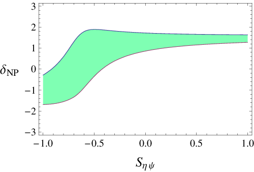

Last, we consider eq. (28). In this case, all the three observables , and are required to constrain .
As a final remark, once experimental information is available about the three observables , and in at least two decay modes , we could constrain also , since only the NP parameters and are channel-specific, while is the same for all the modes induced by the weak transition . Hence, measuring in two channels the six observables and it would be possible to determine , , and .
4 Conclusions
Recent results in the sector require efforts to identify the most promising ways to unveal new physics. We have considered decay channels induced by the transition, using generalized factorization together with symmetry to predict their branching fractions in the Standard Model. Modes with a charmonium state plus , , are interesting, since they are CP eigenstates and do not require angular analyses. In particular, the case of is particularly suitable in view of its easier reconstruction in the mode.
If NP affects the sector, it can either contribute to the induced mixing amplitude, in a channel independent way, modifying the value of the mixing phase with respect to its SM value, or modify the decay amplitudes, in a way that can vary from one channel to the other. In this case, the mixing induced CP asymmetry would no more be equal to and the direct CP asymmetry would differ from zero, conditions which instead hold in the SM or in the case that NP affects only the oscillation process. Both cases can also happen. We have considered a general parametrization of new physics in which the second condition holds, fixing either to the average of CDF and D0 results or to its SM value. We have shown that, with data on the branching ratio and the two CP asymmetries and for a given final state , it will be possible to constrain NP parameters.
Acknowledgments.
FDF thanks A.J. Buras for very useful discussions. This work was supported in part by the EU contract No. MRTN-CT-2006-035482, ”FLAVIAnet”.References
- [1] Updated results can be found at: http://www.utfit.org/UTfit/ and http://ckmfitter.in2p3.fr/.
- [2] A. Abulencia et al. [CDF Collaboration], Phys. Rev. Lett. 97 (2006) 242003.
- [3] V. M. Abazov et al. [D0 Collaboration], Phys. Rev. Lett. 98 (2007) 121801.
- [4] V. M. Abazov et al. [D0 Collaboration], Phys. Rev. Lett. 101 (2008) 241801.
- [5] V. M. Abazov et al. [D0 Collaboration], Phys. Rev. D 76 (2007) 057101; T. Aaltonen et al. [CDF collaboration], Phys. Rev. Lett. 100 (2008) 121803; T. Aaltonen et al. [CDF Collaboration], Phys. Rev. Lett. 100 (2008) 161802.
- [6] E. Barberio et al. [Heavy Flavor Averaging Group], arXiv:0808.1297 [hep-ex].
- [7] L. Oakes (on behalf of the CDF Collaboration), talk given at FPCP 2010, Torino, Italy, 25-29 May 2010.
- [8] V. M. Abazov et al. [The D0 Collaboration], Phys. Rev. D 82 (2010) 032001; Phys. Rev. Lett. 105 (2010) 081801.
- [9] V. M. Abazov et al. [D0 Collaboration], Phys. Rev. D 74 (2006) 092001.
- [10] A. Lenz et al., arXiv:1008.1593 [hep-ph].
- [11] G. Buchalla, A. J. Buras and M. E. Lautenbacher, Rev. Mod. Phys. 68 (1996) 1125.
- [12] K. Nakamura et al. [Particle Data Group], J. Phys. G 37 (2010) 075021.
- [13] M. Neubert and B. Stech, Adv. Ser. Direct. High Energy Phys. 15 (1998) 294.
- [14] A. J. Buras and L. Silvestrini, Nucl. Phys. B 548 (1999) 293.
- [15] Y. Y. Keum, H. n. Li and A. I. Sanda, Phys. Lett. B 504 (2001) 6; Phys. Rev. D 63 (2001) 054008. C. D. Lu, K. Ukai and M. Z. Yang, Phys. Rev. D 63 (2001) 074009.
- [16] M. Beneke, G. Buchalla, M. Neubert and C. T. Sachrajda, Phys. Rev. Lett. 83 (1999) 1914; Nucl. Phys. B 591 (2000) 313.
- [17] A. Khodjamirian, Nucl. Phys. B 605 (2001) 558.
- [18] B. Melic, Phys. Rev. D 68 (2003) 034004; Z. G. Wang, L. Li and T. Huang, Phys. Rev. D 70 (2004) 074006.
- [19] P. Colangelo and A. Khodjamirian, in ”At the Frontier of Particle Physics / Handbook of QCD”, ed. by M. Shifman (World Scientific, Singapore, 2001), vol. 3, pages 1495-1576, arXiv:hep-ph/0010175.
- [20] P. Colangelo, F. De Fazio, P. Santorelli and E. Scrimieri, Phys. Rev. D 53 (1996) 3672 [Erratum-ibid. D 57 (1998) 3186].
- [21] P. Ball and R. Zwicky, Phys. Rev. D 71 (2005) 014015.
- [22] P. Ball and R. Zwicky, Phys. Rev. D 71 (2005) 014029.
- [23] P. Colangelo, F. De Fazio and W. Wang, Phys. Rev. D 81 (2010) 074001.
- [24] T. Feldmann, P. Kroll and B. Stech, Phys. Rev. D 58 (1998) 114006; Phys. Lett. B 449 (1999) 339; T. Feldmann, Int. J. Mod. Phys. A 15 (2000) 159.
- [25] F. Ambrosino et al. [KLOE Collaboration], Phys. Lett. B 648 (2007) 267.
- [26] F. De Fazio and M. R. Pennington, JHEP 0007 (2000) 051.
- [27] I. Adachi et al. [Belle Collaboration], arXiv:0912.1434.
- [28] R. Louvot (on behalf of the Belle Collaboration), arXiv:1009.2605.
- [29] S. Stone and L. Zhang, Phys. Rev. D 79 (2009) 074024; arXiv:0909.5442.
- [30] O. Leitner, J. P. Dedonder, B. Loiseau and B. El-Bennich, arXiv:1003.5980 [hep-ph].
- [31] M. Ablikim et al. [BES Collaboration], Phys. Rev. D 70 (2004) 092002; Phys. Rev. D 72 (2005) 092002.
- [32] P. Colangelo, F. De Fazio and T. N. Pham, Phys. Lett. B 542 (2002) 71; Phys. Rev. D 69 (2004) 054023.
- [33] P. Colangelo, F. De Fazio and T. N. Pham, Phys. Lett. B 597 (2004) 291.