The effect of varying sound velocity on primordial curvature perturbations

Standard inflationary cosmology [1, 2, 3] predicts nearly scale-invariant power spectrum of the primordial perturbation [4, 5, 6, 7]. Such a power-law like perturbation spectrum $\Delta_{\zeta}^{2}\propto k^{n_{s}-1}$, where $\zeta$ is the comoving curvature perturbation and $n_{s}$ is the scalar spectral index with $n_{s}\simeq 1$ has been prefered also from a number of obserbations [8]. If we look into the detailed structure of the Cosmic Microwave Background (CMB) temperature anisotropy, some hints of small deviations from the simplest form of the curvature perturbation power spectrum show up. Among those, anomalously low values of the quadrupole moment or several sharp glitches in the large scale WMAP data corresponing to $\ell\sim 20-40$ are famous and most intensively studied [9]. Furthermore, several groups have reported strong evidence of the deviation from a simple power-law type power spectrum by reconstructing the primordial power spectrum from the WMAP data [10, 11, 12, 13, 14, 15, 16, 17, 18, 19]. In particular, Ichiki et al. [20, 21] claim that they found an oscillatory modulation localized around the comoving wavenumber $k\simeq 0.009[\mathrm{Mpc}^{-1}]$ ($\ell\simeq 120$) in the power spectrum at 99.995$\%$ confidence level.

Theoretical calculation for the power spectrum has been also sophisticated recently and some inflation models based on a realistic high-energy physics can generate peculiar features on the curvature perturbation. Those include the so-called Trans-Planckian effect [22, 23, 24], particle production due to the coupling between the inflaton and another scalar filed [25, 26, 27], temporal violation of the slow-rolling of the inflaton field [28, 29, 30, 31, 32, 33, 34, 35], and some other models [36, 37]. To go further into the accurate cosmology, it is crucial to study further the details of the primordial perturbations. This leads us to the detailed structure of the inflaton Lagrangian or the true high-energy physics that has realized in our Universe.

In this paper, we concentrate on the role of the sound velocity, which is defined as the propagating speed of the linear perturbation in the next section. In some high-energy physics theories, there appear non-canonical kinetic terms in the Lagrangian and in that case the sound velocity deviates from unity [38, 39]. Furthermore, if those kinetic terms of the inflaton field couple to some time-dependent variables which can be seen, for example, in DBI inflation scenario [40], the values of the sound velocity can change during inflation [41, 42, 43]. Then we have to consider the possibility of some non-trivial dynamics of the perturbation. As a result, new degrees of freedom such as the sound velocity may be observed in the CMB temperature fluctuation and be tested in the future high-precision CMB observations such as PLANCK or CMBpol.

This paper is organized as follows. In the next section, we comment on the background evolution in our scenario and introduce the sound velocity. In sec III, the basic variables and its evolution equation for the curvature perturbation are described. Then we consider the paricular types of the variation of the sound velocity. The first type is a step-like function, which is discussed in Sec. IV, and the second type is a top-hat type function, which we will study in Sec. V. The last section is devoted to the summury and discussion.

In the standard single inflaton field with a canonical kinetic term, the sound velocity $c_{s}$ defined by the propagation speed of linear perturbation has the value equal to the speed of light, namely, $c_{s}=1$. This is easily checked by considering the action of the canonical inflaton field,

$$S=\int d^{4}x\sqrt{-g}\left(\frac{1}{2}R+X+V(\phi)\right),\ \ X=-{1\over 2}g^{\mu\nu}\partial_{\mu}\phi\partial_{\nu}\phi,$$

(1)

where $R$ denote the Einstein-Hilbert action and we set the reduced Planck scale to unity ($8\pi G=1$). Expanding the action around the background Friedman-Robertson-Walker (FRW) metric up to second-order, then we can see that the sound velocity which appears as the coefficient of the spatial derivative term is exactly equal to one.

Generalizing the above inflaton action to an arbitary function of the kinetic term $X$,

$$S=\int d^{4}x\sqrt{-g}\left(\frac{1}{2}R+P(X,\phi)\right),$$

(2)

the situation changes completely. In this action, expanding around FRW metric up to second-order, we find the sound velocity is given by

$\displaystyle c_{s}^{2}=\frac{P_{X}}{2P_{XX}X+P_{X}},$

(3)

where the subscript $X$ represents a derivative with respect to $X$. The specific second-order action for the approapriate perturbation variable, what we call the comoving curvature perturbation, will be presented in the next section. It is clear from (3) that, in principle, the sound velocity takes various values corresponding to the functional form $P(X,\phi)$ and the values of $X$ and $\phi$.

In this paper, in order to extract the effects of the change of the sound velocity alone, we study the cases it changes suddenly once or twice during inflation without affecting the background evolution. The sudden change of the sound velocity can be realized, for example, if the Lagrangian has terms like

$$P(X,\phi)\supset f(\phi)X+[1-f(\phi)]X^{2}/\Lambda^{4},\ \ f(\phi)=\frac{1}{1+e^{(\phi-\phi_{0})/d}},$$

(4)

or

$$P(X,\phi)\supset b(\phi)X+X^{2}/\Lambda^{4},\ \ b(\phi)\simeq(\phi-\phi_{0})^{2}+\mathcal{O}\left((\phi-\phi_{0})^{n}\right),\ \ \ (n\geq 3)$$

(5)

where $\phi$ is a scaler field which we assume to be the inflaton and $\Lambda$ is some cut-off scale. In the former case, we find $c_{s}^{2}=1$ when $\phi\ll\phi_{0}$ and $c_{s}^{2}=1/3$ when $\phi\gg\phi_{0}$. Such a transition of the sound velocity due to the motion of the field $\phi$ is approximately described by a step function. In the latter case, $c_{s}^{2}=1/3$ only when $\phi\simeq\phi_{0}$ and at the other values of $\phi$, $c_{s}^{2}=1$. This variation is well approxmated by a top-hat type function. In generic unified theories including string theory, there appears many scalar fields which have non-trivial kinetic terms and it is likely that those kinetic terms naturally couple to the scalar field itself in a complicated way. Here we consider simple tractable examples of posssible deviation from the canonical model as described above.

If we take these models as they are, the background evolution, in particular the slow-roll parameters, may also be severely modulated unless some fine-tunning is applied. Since the effects of the sudden change of slow-roll parameters

$$\epsilon=-\frac{\dot{H}}{H^{2}},\ \ \ \eta=\frac{\dot{\epsilon}}{H\epsilon},$$

(6)

where a dot represents a derivative with respect to the physical time $t$, have been already studied in the literatures [31, 32], we concentrate on the cases only the sound velocity changes suddenly as mentioned above. Thus, we impose the slow-roll conditions

$$|\epsilon|\ll 1,\ \ \ |\eta|\ll 1,$$

(7)

throughout this paper. Such a situation can be also realized in the curvaton scenario as discussed in Appendix A.

In the usual calculation of linear perturbation in this type of generalized non-canonical kinetic term inflation models, new parameters which parametrize the time variation of the sound velocity such as

$\displaystyle\epsilon_{s}={\dot{c}_{s}\over c_{s}H},\ \ \ \eta_{s}={\dot{\epsilon}_{s}\over\epsilon_{s}H},$

(8)

are introduced and additional slow-roll conditions $|\epsilon_{s}|<1,|\eta_{s}|<1$ are imposed. In this paper, however, being interested in the effect of the more general variation of sound velocity mentioned above, we consider the situation where these conditions are temporarily violated by the sudden change of the sound velocity.

In the following sections, we derive the approapriate variables for calculating the perturbation and the matching condition at the transition epoch. Then we evaluate the final power spectrum for two concrete examples of the sound velocity variation.

The scalar perturbation from the Background FRW metric in the conformal Newtonian gauge is incorporated as

$$ds^{2}=a^{2}\left[-(1+2\Psi)d\tau^{2}+(1+2\Phi)\delta_{ij}dx^{i}dx^{j}\right]$$

(9)

Denoting the inflaton perturbation $\delta\phi$ and the background value of the inflaton field $\bar{\phi}$, the most common perturbation variable, namely, comoving curvature perturbation $\zeta$ is defined as [44, 45, 46]

$$\zeta\equiv\Phi+\frac{H}{\dot{\bar{\phi}}}\delta\phi.$$

(10)

The basic action and the equation of motion in the linear theory for $\zeta$ is written in terms of

$$v=\zeta z,$$

(11)

where a new parameter $z$ is defined by

$\displaystyle z\equiv\frac{a\sqrt{2\epsilon}}{c_{s}}.$

(12)

The second-order action for $v$ is derived by substituting (9) and $\phi=\bar{\phi}+\delta\phi$ into (2), neglecting the higher-order terms and using the background evolution equation. The result is

$$S^{(2)}=\frac{1}{2}\int d\tau d^{3}x\left(v^{\prime 2}+c_{s}^{2}v\Delta v+\frac{z^{\prime\prime}}{z}v^{2}\right),$$

(13)

where a prime denotes a derivative with respect to the conformal time $\tau$. Then, the equation of motion for Fourier-transformed perturbation variable $v_{k}$ is given by

$$v_{k}^{\prime\prime}+\left(c_{s}^{2}k^{2}-\frac{z^{\prime\prime}}{z}\right)v_{k}=0.$$

(14)

The above so-called Mukhanov-Sasaki equation (14) is commonly used to discuss the behavior of the curvature perturbation. Here, however, we are interested in the time-dependence of the sound velocity, in which situation the potential term $z^{\prime\prime}/z$ in (14) is not easy to treat since the variable $z$ also contains $c_{s}$. For example, if we consider a step-function-type variation of the sound velocity, a square term of $(c_{s}^{\prime}/c_{s})$ appears in $z^{\prime\prime}/z$, which becomes the square of the delta function $\delta(\tau-\tau_{0})$ and makes the analysis impossible where $\tau_{0}$ denotes time when sound velocity changes.

It is therefore clear that the equation for $v_{k}$ is not suitable¹¹ 1 As discussed in Appendix A, this is not the case in the curvaton scenario. and so we should introduce a new variable $u_{k}$, which is related to $v_{k}$ as [47]

$$-c_{s}k^{2}u_{k}=z\left(\frac{v_{k}}{z}\right)^{\prime},\ \ c_{s}v_{k}=\theta\left(\frac{u_{k}}{\theta}\right)^{\prime},$$

(15)

where we have defined

$$\theta\equiv\frac{1}{c_{s}z}.$$

(16)

The basic equation of motion (14) for $v_{k}$ is translated into the new equation in terms of $u_{k}$, which is

$$u_{k}^{\prime\prime}+\left(c_{s}^{2}k^{2}-\frac{\theta^{\prime\prime}}{\theta}\right)u_{k}=0.$$

(17)

Note that the term $(c_{s}^{\prime}/c_{s})$ does not exist in $\theta^{\prime\prime}/\theta$ since the variable $\theta$ does not depend on $c_{s}$ due to the definition of $\theta$, (16). We have to solve this equation under the assumption that the background evolution satisfies the slow-roll conditions (7).

The term $\theta^{\prime\prime}/\theta$ is rewritten in terms of slow-roll parameters as

$\displaystyle\frac{\theta^{\prime\prime}}{\theta}=\frac{1}{\tau^{2}}\left(\frac{\eta}{2}+\epsilon\right),$

(18)

where we have used slow-roll approximation (7) and a useful equation

$$aH=-\frac{1}{\tau(1-\epsilon)}.$$

(19)

Therefore, we obtain the basic equation as

$$u_{k}^{\prime\prime}+\left(c_{s}^{2}k^{2}-\frac{\nu^{2}-\frac{1}{4}}{\tau^{2}}\right)u_{k}=0,$$

(20)

where we have defined

$$\nu^{2}=\frac{\eta}{2}+\epsilon+\frac{1}{4}.$$

(21)

and approximate it as

$$\nu=\sqrt{\frac{\eta}{2}+\epsilon+\frac{1}{4}}\approx\frac{1}{2}+\frac{\eta}{2}+\epsilon.$$

(22)

In this section, we compute the curvature perturbation for a model such that time variation of the sound velocity is described by a step function as

$\displaystyle c_{s}=\begin{cases}c_{s1}&(\tau<\tau_{0})\\ c_{s2}&(\tau>\tau_{0})\end{cases}.$

(23)

To take into account the transition of the sound velocity, it is important to impose a matching condition to the solution in (17) at $\tau=\tau_{0}$ when the sound velocity suddenly changes. The matching condition is obtained by integrating (17) in an infinitesimaly small time interval $[\tau_{0}-\delta\tau,\tau_{0}+\delta\tau]$, yielding two conditions;

$$u_{k}(\tau_{0}-\delta\tau)=u_{k}(\tau_{0}+\delta\tau),\ \ u_{k}^{\prime}(\tau_{0}-\delta\tau)=u_{k}^{\prime}(\tau_{0}+\delta\tau).$$

(24)

Hereafter, we use the following expression

$$u_{k}(\tau_{0}-\delta\tau)\to u_{k1},\ \ u_{k}(\tau_{0}+\delta\tau)\to u_{k2}.$$

(25)

In the regime when $\tau<\tau_{0}$, setting $c_{s}=c_{s1}$ leads to the equation of motion

$$u_{k}^{\prime\prime}+\left(c_{s1}^{2}k^{2}-\frac{\nu^{2}-\frac{1}{4}}{\tau^{2}}\right)u_{k}=0,$$

(26)

and its solution is obtained by

$$u_{k1}=\sqrt{-kc_{s1}\tau}\left[d_{1}H_{\nu}^{(1)}(-kc_{s1}\tau)+d_{2}H_{\nu}^{(2)}(-kc_{s1}\tau)\right],$$

(27)

where $H_{\nu}^{(1),(2)}(-kc_{s1}\tau)$ denote the Hankel functions and $d_{1,2}$ are constants to be determined by the initial condition at $\tau\to-\infty$. We choose the adiabatic vacuum at the initial time in terms of $v_{k}$:

$$v_{k}\to\frac{1}{\sqrt{2kc_{s1}}}e^{-ikc_{s1}\tau}.$$

(28)

From the equation (15), we find

$\displaystyle-c_{s1}k^{2}u_{k1}=v_{k}^{\prime},$

(29)

well inside the horizon, so we can take

$$u_{k1}=\frac{i}{\sqrt{2c_{s1}}k^{3/2}}e^{-ikc_{s1}\tau}$$

(30)

and match it with the limiting form of the Hankel function,

$$H_{\nu}^{(1,2)}(x)\to\sqrt{\frac{2}{\pi x}}\exp\left[i\left(\pm x-\frac{\nu\pi}{2}-\frac{\pi}{4}\right)\right],\ \ \ (x\to\infty),$$

(31)

where the upper and lower signs correspond to the first and the second types, respectively. Hence it leads to the choice of $d_{1},d_{2}$ as

$$d_{1}=\frac{i}{2k^{3/2}}\sqrt{\frac{\pi}{c_{s1}}}\exp\left(\frac{2\nu+1}{4}\pi i\right),\ \ \ d_{2}=0.$$

(32)

Neglecting all the phase factors which is irrelevant for calculating the power spectrum, the solution $u_{k1}$ takes the form

$$u_{k1}=\frac{\sqrt{-\pi\tau}}{2k}H_{\nu}^{(1)}(-kc_{s1}\tau).$$

(33)

Next, in the regime when $\tau>\tau_{0}$, setting $c_{s}=c_{s2}$ leads to

$\displaystyle u_{k2}=\frac{\sqrt{-kc_{s2}\tau}}{2}\left[\alpha_{k}^{\prime}H_{\nu}^{(1)}(-kc_{s2}\tau)+\beta_{k}^{\prime}H_{\nu}^{(2)}(-kc_{s2}\tau)\right],$

(34)

and it is rewritten by

$\displaystyle u_{k2}=\frac{\sqrt{-\pi\tau}}{2k}\left[\alpha_{k}H_{\nu}^{(1)}(-kc_{s2}\tau)+\beta_{k}H_{\nu}^{(2)}(-kc_{s2}\tau)\right],$

(35)

where we have defined

$$\alpha_{k}\equiv\sqrt{\frac{c_{s2}}{\pi}}k^{3/2}\alpha_{k}^{\prime},\ \ \ \beta_{k}\equiv\sqrt{\frac{c_{s2}}{\pi}}k^{3/2}\beta_{k}^{\prime}.$$

(36)

From (24), we finally obtain the coefficients $\alpha_{k}$ and $\beta_{k}$ as

	$\displaystyle\alpha_{k}$	$\displaystyle=\frac{i\pi k\tau_{0}}{4}\left[c_{s2}H_{\nu}^{(1)}(-kc_{s1}\tau_{0})H_{\nu+1}^{(2)}(-kc_{s2}\tau_{0})-c_{s1}H_{\nu}^{(2)}(-kc_{s2}\tau_{0})H_{\nu+1}^{(1)}(-kc_{s1}\tau_{0})\right],$		(37)
	$\displaystyle\beta_{k}$	$\displaystyle=-\frac{i\pi k\tau_{0}}{4}\left[c_{s2}H_{\nu}^{(1)}(-kc_{s1}\tau_{0})H_{\nu+1}^{(1)}(-kc_{s2}\tau_{0})-c_{s1}H_{\nu}^{(1)}(-kc_{s2}\tau_{0})H_{\nu+1}^{(1)}(-kc_{s1}\tau_{0})\right],$		(38)

where we have used the following relation among the Hankel functions,

$\displaystyle H_{\nu+1}^{(1)}(x)H_{\nu}^{(2)}(x)-H_{\nu+1}^{(2)}(x)H_{\nu}^{(1)}(x)=-{4i\over\pi x}.$

(39)

We have to estimate the power spectrum of $\zeta$ at the final time $\tau\to 0$. By using (15), the curvature perturbation can be rewritten in terms of the variable $u$ as

	$\displaystyle\zeta_{k}$	$\displaystyle=\frac{v_{k}}{z}=\theta^{2}\left(\frac{u_{k}}{\theta}\right)^{\prime}=\theta\left(u_{k}^{\prime}-\frac{\theta^{\prime}}{\theta}u_{k}\right)$
		$\displaystyle\approx\frac{H}{\sqrt{2\epsilon}}\left(1-\frac{\eta}{2}\right)u_{k}.$		(40)

where, at the last transformation, we have chosen the super-horizon limit and neglected $u_{k}^{\prime}$ term. Therefore, we need the final values expressed as $u_{k2}(\tau\to 0)$. From the solution (35), we obtain

$\displaystyle u_{k2}(\tau\to 0)$

$\displaystyle\simeq\frac{\sqrt{-\pi\tau}}{2k}\frac{i}{\pi}\Gamma(\nu)\left(\frac{-kc_{s2}\tau}{2}\right)^{-\nu}(\alpha_{k}-\beta_{k}),$

(41)

where $\Gamma(x)$ denotes the Gamma function and we have used the limiting form of the Hunkel function as

$$H_{\nu}^{(1)}(y)\simeq-H_{\nu}^{(2)}(y)\simeq\frac{i}{\pi}\Gamma(\nu)\left(\frac{y}{2}\right)^{-\nu},\ \ \ (y\to 0).$$

(42)

By using (40) and (41), we can calculate the power spectrum of curvature perturbation as

$\displaystyle P_{\zeta}(k)=|\zeta_{k}(\tau\to 0)|^{2}\approx{4^{\nu}\Gamma^{2}(\nu)\over 8\pi k^{2}}{H^{2}\over\epsilon}\left[aH(1-\epsilon)\right]^{2\nu-1}(kc_{s2})^{-2\nu}\left(1+\eta\right)|\alpha_{k}-\beta_{k}|^{2}+\mathcal{O}(\epsilon^{2},\eta^{2}),$

(43)

where we have used the slow-roll approximation. Hence the term $|\alpha_{k}-\beta_{k}|^{2}$ is important to determine the power spectrum. $\alpha_{k}-\beta_{k}$ can be described by using (37) and (38) as

	$\displaystyle\alpha_{k}-\beta_{k}$	$\displaystyle=\frac{i\pi k\tau_{0}}{2}\biggl[\Bigl(c_{s2}J_{\nu}(-kc_{s1}\tau_{0})J_{\nu+1}(-kc_{s2}\tau_{0})-c_{s1}J_{\nu+1}(-kc_{s1}\tau_{0})J_{\nu}(-kc_{s2}\tau_{0})\Bigr)$
		$\displaystyle\ \ \ \ \ \ +i\Bigl(c_{s2}N_{\nu}(-kc_{s1}\tau_{0})J_{\nu+1}(-kc_{s2}\tau_{0})-c_{s1}N_{\nu+1}(-kc_{s1}\tau_{0})J_{\nu}(-kc_{s2}\tau_{0})\Bigr)\biggr],$		(44)

where $J_{\nu},N_{\nu}$ are the Bessel functions with $\nu={1\over 2}+{\eta\over 2}+\epsilon$. Then we can calculate $|\alpha_{k}-\beta_{k}|^{2}$ as

	$\displaystyle|\alpha_{k}-\beta_{k}|^{2}$	$\displaystyle=\frac{\pi^{2}k^{2}\tau_{0}^{2}}{4}\biggl[\Bigl(c_{s2}J_{\nu}(-kc_{s1}\tau_{0})J_{\nu+1}(-kc_{s2}\tau_{0})-c_{s1}J_{\nu+1}(-kc_{s1}\tau_{0})J_{\nu}(-kc_{s2}\tau_{0})\Bigr)^{2}$
		$\displaystyle\ \ \ \ \ \ +\Bigl(c_{s2}N_{\nu}(-kc_{s1}\tau_{0})J_{\nu+1}(-kc_{s2}\tau_{0})-c_{s1}N_{\nu+1}(-kc_{s1}\tau_{0})J_{\nu}(-kc_{s2}\tau_{0})\Bigr)^{2}\biggr].$		(45)

Here, we define new variables $A$ and $k_{0}$ as

$$c_{s2}=Ac_{s1},\ \ -c_{s2}\tau_{0}=\frac{1}{k_{0}},\ \ -c_{s1}\tau_{0}=\frac{1}{Ak_{0}},$$

(46)

and using them leads to

	$\displaystyle|\alpha_{k}-\beta_{k}|^{2}$	$\displaystyle=\frac{\pi^{2}k^{2}}{4k_{0}^{2}A^{2}}\bigg\{A^{2}J_{\nu+1}^{2}\left(\frac{k}{k_{0}}\right)\left[J_{\nu}^{2}\left(\frac{k}{Ak_{0}}\right)+N_{\nu}^{2}\left(\frac{k}{Ak_{0}}\right)\right]+J_{\nu}^{2}\left(\frac{k}{k_{0}}\right)\left[J_{\nu+1}^{2}\left(\frac{k}{Ak_{0}}\right)+N_{\nu+1}^{2}\left(\frac{k}{Ak_{0}}\right)\right]$
		$\displaystyle\ \ \ \ \ \ -2AJ_{\nu+1}\left(\frac{k}{k_{0}}\right)J_{\nu}\left(\frac{k}{k_{0}}\right)\left[J_{\nu}\left(\frac{k}{Ak_{0}}\right)J_{\nu+1}\left(\frac{k}{Ak_{0}}\right)+N_{\nu}\left(\frac{k}{Ak_{0}}\right)N_{\nu+1}\left(\frac{k}{Ak_{0}}\right)\right]\bigg\}.$		(47)

Finally, we can evaluate the power spectrum at the sound horizon crossing $aH=kc_{s2}$ as

$\displaystyle P_{\zeta}(k)={2^{1+\eta+2\epsilon}\over 8\pi}\Gamma^{2}\left({1\over 2}+{\eta\over 2}+\epsilon\right){(1-\epsilon)^{\eta+2\epsilon}\over\epsilon}{H^{2}\over k^{3}}\left(1+\eta\right)|\alpha_{k}-\beta_{k}|^{2}\bigg|_{aH=kc_{s2}}.$

(48)

In the lowest-order slow-roll approxmation, we can set $\nu={1\over 2}$, in which case the Bessel functions are expressed by trigonometric functions and the modulation factor $|\alpha_{k}-\beta_{k}|^{2}$ can be recast to the following simple form (see Fig.1(a)).

$\displaystyle|\alpha_{k}-\beta_{k}|^{2}=A\left[1+\left(\frac{1}{A^{2}}-1\right)\sin^{2}\left(\frac{k}{k_{0}}\right)\right].$

(49)

In this case, neglecting the slow-roll correction in the numerator, the dimensionless power spectrum (48) becomes

$$\Delta^{2}_{\zeta}(k)\equiv{k^{3}\over 2\pi^{2}}P_{\zeta}(k)={H^{2}A\over 8\pi^{2}\epsilon c_{s2}}\left[1+\left(\frac{1}{A^{2}}-1\right)\sin^{2}\left(\frac{k}{k_{0}}\right)\right].$$

(50)

This result recovers the usual power spectrum with constant sound velocity if we take $A=1$. In the large-scale limit $k\to 0$, we can drop the oscillatory term and the final expression becomes

$$\Delta^{2}_{\zeta}(k)={H^{2}\over 8\pi^{2}\epsilon c_{s1}},$$

(51)

which represents the power spectrum for modes which cross the horizon far before the transition time $\tau_{0}$.

Taking the result (50) as the input primordial power specrum, or more quantitatively speaking, taking

	$$\displaystyle\Delta^{2}_{\zeta}(k)=A_{s}\left(\frac{k}{k_{piv}}\right)^{n_{s}-1}\left[1+A_{mp}\sin^{2}\left(\frac{k}{k_{0}}\right)\right],$$		(52)
	$$\displaystyle A_{s}=2.43\times 10^{-9},\ k_{piv}=0.002[\mathrm{Mpc}^{-1}],\ n_{s}=0.963,$$

as the input one, we have computed CMB temperature anisotropy for several values of $k_{0}$ (see Fig.1(b)). Comparing (52) with (50), we can clearly see that $A_{mp}\equiv 1/A^{2}-1$. The parameter $k_{0}$ determines the scale under which the rapid modulation appears. As we expect, if the value of $k_{0}$ is chosen as $\mathcal{O}(0.001[\mathrm{Mpc}^{-1}])$ or smaller, then the CMB spectrum starts to oscillate at the relatively large scale around $\ell\simeq 10$, which may better fit some anomalous data points obserbed in WMAP. Actually, as one exapmle value, if we take $k_{0}=0.003[\mathrm{Mpc}^{-1}]$, $A_{mp}=0.087$ and neglect the small scale ($\ell\geq 200)$ oscillation, we have found that the $\chi^{2}$-value improves $3.2$ compared with the usual case of power-law primordial power spectrum.

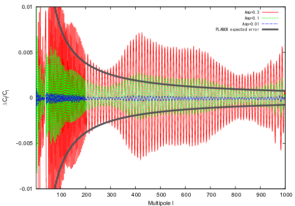
In Fig.2, we have plotted the difference between the CMB temperature anisotropy spectrum calculated by the primordial power spectrum with oscillations (52) and the one by the usual power-law power spectrum without oscillations, which we denote $C_{\ell}^{osc}$ and $C_{\ell}^{std}$, respectively. Here the difference is defined as

$$\frac{\Delta C_{\ell}}{C_{\ell}}\equiv\frac{C_{\ell}^{osc}-C_{\ell}^{std}}{C_{\ell}^{std}}.$$

(53)

Note that the overall amplitude $A_{s}$ in $C_{\ell}^{osc}$ is different from that used in $C_{\ell}^{std}$ by a factor $(1+A_{mp}/2)^{-1}$. We have also plotted the expected scatter of $C_{\ell}$ due to the cosmic variance, which is given by

$$\left(\frac{\Delta C_{\ell}}{C_{\ell}}\right)_{\mathrm{CV}}=\sqrt{\frac{2}{(2\ell+1)f_{sky}}},\ \ f_{sky}=0.65.$$

(54)

Note that the observational error of WMAP is cosmic-variance limited up to $\ell\simeq 400$ and it will be extended to $\ell\simeq 2500$ for PLANCK. Hence from this figure we can constrain $A_{mp}$ as $A_{mp}\lesssim 0.1$ now for $k_{0}=10^{-4}[\mathrm{Mpc}^{-1}]$ which corresponds to the largest scale that can be measured with CMB experiments.

This feature in the spectrum can be compared with the Trans-Planckian signatures [22, 23, 24], with the particle production effect, or with the spectrum generated in the case the inflaton potential has a break in its slope. In the first case, the modification of the initial vacuum can change the relation and then leads to the ringing signatures in the primordial power spectrum. The exact form of the pattern depends on the choice of the hypersurface on which the initial condition is imposed. In the so-called Boundary Effective Field Theory (BEFT) approach [48, 49], the final expression becomes

$$\mathcal{P}_{\mathrm{BEFT}}(k)=A_{s}\left(\frac{k}{k_{0}}\right)^{n_{s}-1}\left[1+\frac{\beta k}{a_{i}\Lambda}\sin\left(2\frac{k}{a_{i}{H_{i}}}\right)\right]$$

(55)

where $a_{i}$ and $H_{i}$ are the scale factor and the Hubble parameter on the initial condition hypersurface, respectively, and $\Lambda$ is a cutoff scale. This is similar to our result (50), but the amplitude of the oscillation depends on the wavenumber $k$, which makes crucial difference with our result.

In the second case, Barnaby et al. [26] discuss that the particle production (PP) make a bumplike contribution to the power spectrum, which is well fitted by

$$\mathcal{P}_{\mathrm{PP}}(k)=A_{s}\left(\frac{k}{k_{0}}\right)^{n_{s}-1}+A_{\star}\left(\frac{k}{k_{\star}}\right)^{3}\exp\left(-\frac{\pi k^{2}}{2k_{\star}^{2}}\right).$$

(56)

The feature is localized around $k_{\star}$, which makes sharp difference with our result.

In the last category, where the second derivative of the inflaton field has a sudden change at $\tau=\tau_{0}$, the modulation factor can be calculated similarly and the final expression is also similar to our result at the first glance. However, there is a big difference because in this case the slow-roll parameter has a step-like function over the transition time and the tilt of the spectrum takes the different values before and after the transition [33, 34].

In this section, we consider the other type of variation of sound velocity, namely, the top-hat type. This is a simple extension of the model discussed in the last section. We parametrize the variation as

$\displaystyle c_{s}=\begin{cases}c_{s1}&(\tau<\tau_{0})\\ c_{s2}&(\tau_{0}<\tau<\tau_{0}^{\prime})\\ c_{s1}&(\tau_{0}^{\prime}<\tau)\end{cases}.$

(57)

and impose the same matching condition to the wavefunction $u_{k}$ as in (24) at the two transition times $\tau_{0}$ and $\tau_{0}^{\prime}$. The solutions of the equation of motion during constant sound velocity regimes are expressed in the same way as in the last section and we parametrize them as follows;

	$\displaystyle u_{k1}$	$\displaystyle=P\frac{\sqrt{-\pi\tau}}{2k}H_{\nu}^{(1)}(-kc_{s1}\tau)\ \ (\tau<\tau_{0}),$		(58)
	$\displaystyle u_{k2}$	$\displaystyle=\frac{\sqrt{-\pi\tau}}{2k}\left[\alpha_{k1}H_{\nu}^{(1)}(-kc_{s2}\tau)+\beta_{k1}H_{\nu}^{(2)}(-kc_{s2}\tau)\right]\ \ (\tau_{0}<\tau<\tau_{0}^{\prime}),$		(59)
	$\displaystyle u_{k3}$	$\displaystyle=\frac{\sqrt{-\pi\tau}}{2k}\left[\alpha_{k2}H_{\nu}^{(1)}(-kc_{s1}\tau)+\beta_{k2}H_{\nu}^{(2)}(-kc_{s1}\tau)\right]\ \ (\tau_{0}^{\prime}<\tau),$		(60)

where we have chosen the Bunch-Davies vacuum state at $\tau\ll\tau_{0}$. Two coefficients $\alpha_{k1}$ and $\beta_{k1}$ in (59) correspond to $\alpha_{k}$ and $\beta_{k}$ in (35). Since the solutions and the matching conditions are the same, the coefficients $\alpha_{k1}$ and $\beta_{k1}$ are given by (37) and (38). The matching conditions at $\tau=\tau_{0}^{\prime}$ gives the relations between $\alpha_{k2},\beta_{k2}$ and $\alpha_{k1},\beta_{k1}$;

	$\displaystyle\alpha_{k2}$	$\displaystyle=-\frac{i\pi k\tau_{0}^{\prime}}{4}\Bigg[\bigg\{c_{s2}H_{\nu+1}^{(1)}(-kc_{s2}\tau_{0}^{\prime})H_{\nu}^{(2)}(-kc_{s1}\tau_{0}^{\prime})-c_{s1}H_{\nu+1}^{(2)}(-kc_{s1}\tau_{0}^{\prime})H_{\nu}^{(1)}(-kc_{s2}\tau_{0}^{\prime})\bigg\}\alpha_{k1}$
		$\displaystyle\ \ \ \ +\bigg\{c_{s2}H_{\nu+1}^{(2)}(-kc_{s2}\tau_{0}^{\prime})H_{\nu}^{(2)}(-kc_{s1}\tau_{0}^{\prime})-c_{s1}H_{\nu+1}^{(2)}(-kc_{s1}\tau_{0}^{\prime})H_{\nu}^{(2)}(-kc_{s2}\tau_{0}^{\prime})\bigg\}\beta_{k1}\Bigg],$		(61)
	$\displaystyle\beta_{k2}$	$\displaystyle=\frac{i\pi k\tau_{0}^{\prime}}{4}\Bigg[\bigg\{c_{s2}H_{\nu+1}^{(1)}(-kc_{s2}\tau_{0}^{\prime})H_{\nu}^{(1)}(-kc_{s1}\tau_{0}^{\prime})-c_{s1}H_{\nu+1}^{(1)}(-kc_{s1}\tau_{0}^{\prime})H_{\nu}^{(1)}(-kc_{s2}\tau_{0}^{\prime})\bigg\}\alpha_{k1}$
		$\displaystyle\ \ \ \ +\bigg\{c_{s2}H_{\nu+1}^{(1)}(-kc_{s2}\tau_{0}^{\prime})H_{\nu}^{(1)}(-kc_{s1}\tau_{0}^{\prime})-c_{s1}H_{\nu+1}^{(1)}(-kc_{s1}\tau_{0}^{\prime})H_{\nu}^{(1)}(-kc_{s2}\tau_{0}^{\prime})\bigg\}\beta_{k1}\Bigg].$		(62)

We want to know the power spectrum of the curvature perturbation at the final epoch $\tau\to 0$. As we have already seen, all we need is $u_{k3}(\tau\to 0)$. Combination of the solution (60) and the limiting form of the Hankel function leads to

$\displaystyle u_{k3}(\tau\to 0)$

$\displaystyle\simeq\frac{\sqrt{-\pi\tau}}{2k}\frac{i}{\pi}\Gamma(\nu)\left(\frac{-kc_{s1}\tau}{2}\right)^{-\nu}(\alpha_{k2}-\beta_{k2}),$

(63)

and the power spectrum of the curvature perturbation is described as

$$P_{\zeta}(k)\equiv|\zeta(\tau\to 0)|^{2}=\frac{H^{2}}{2\epsilon}\left(1+\frac{\eta}{2}\right)^{2}|u_{k3}(\tau\to 0)|^{2}.$$

(64)

Also in this case, the factor to determine the modulation pattern is $|\alpha_{k2}-\beta_{k2}|^{2}$, which can be calculated by inserting (37) and (38) into (61) and (62). The final functional form however is so complicated. We therefore show the result only in the leading order slow-roll approximaton;

	$\displaystyle|\alpha_{k2}-\beta_{k2}|^{2}$	$\displaystyle\simeq\cos^{2}\left[-kc_{s2}(\tau_{0}^{\prime}-\tau_{0})\right]+\sin^{2}\left[-kc_{s2}(\tau_{0}^{\prime}-\tau_{0})\right]\left[A^{2}\sin^{2}(-kc_{s1}\tau_{0}^{\prime})+\frac{1}{A^{2}}\cos^{2}(-kc_{s1}\tau_{0}^{\prime})\right]$
		$\displaystyle\ \ \ \ -2\left(A-\frac{1}{A}\right)\cos(-kc_{s1}\tau_{0}^{\prime})\sin(-kc_{s1}\tau_{0}^{\prime})\cos\left[-kc_{s2}(\tau_{0}^{\prime}-\tau_{0})\right]\sin\left[-kc_{s2}(\tau_{0}^{\prime}-\tau_{0})\right]+\mathcal{O}(\epsilon,\eta).$		(65)

As expected, the modulation is determined by the combination of sine and cosine osillations. We can transform (65) to the following form.

	$\displaystyle|\alpha_{k2}-\beta_{k2}|^{2}=$	$\displaystyle 1-\frac{A^{2}-1}{2A}\bigg[(A^{2}-1)\sin^{2}\left[-kc_{s2}(\tau_{0}^{\prime}-\tau_{0})\right]-(A^{2}+1)\sin^{2}(-kc_{s1}\tau_{0}^{\prime})$
		$\displaystyle+\frac{(A+1)^{2}}{2}\sin^{2}\left[-kc_{s1}\tau_{0}^{\prime}+kc_{s2}(\tau_{0}^{\prime}-\tau_{0})\right]+\frac{(A-1)^{2}}{2}\sin^{2}\left[-kc_{s1}\tau_{0}^{\prime}-kc_{s2}(\tau_{0}^{\prime}-\tau_{0})\right]\bigg].$		(66)

It is clear in this expression that there is no modulation when $A=1$ or $\tau_{0}=\tau_{0}^{\prime}$, which means no change in sound velocity. If we consider the long-wavelength limit ($k\to 0$), the dimensionless power spectrum of the curvature perturbation reduces to the same form as (51) in the lowest-order slow-roll approximation of the numerator, which is valid because the long-wavelength mode exits the Hubble horizen when the sound velocity is $c_{s1}$ and superhorizen mode does not feel the sound velocity change.

The modulation factor (65) or (66) is plotted in Fig.3(a) and the CMB temperature anisotropy spectrum is plotted in Fig.3(b). In both figures, we defined three parameters $k_{0}$, $A$ and $B$ as $-c_{s1}\tau_{0}^{\prime}=1/k_{0}$, $\tau_{0}=B\tau_{0}^{\prime}$ and $c_{s2}=Ac_{s1}$, respectively. In these figures, We can see a beat, which is very natural because we now have two charactarizing parameters $c_{s1}\tau_{0}^{\prime}$ and $c_{s2}(\tau_{0}^{\prime}-\tau_{0})$ that determines the ocsillation periods and the final modulation pattern is the superposition of these waves. This result is easily extended to more general cases; if the variation of the sound velocity occurs suddenly and during it remains constant at other regimes, then the modulation of the power spectrum is some superpositions of several waves composed by trigonometric functions, which appears as a beat and the amplitude of the oscillation is independent of the wavenumber.

In summary, we have calculated the power spectrum of the curvature perturbation in case the sound velocity changes suddenly during inflation. In order to focus on the effects of the change of the sound velocity, we have assumed that the slow-roll parameters that reflect the background evolution are not affected and remains constant during the transition of the sound velocity and found that in the shorter-wavelength modes (with larger $k$) compared with the Hubble radius at the transition time there appears osillation patterns due to the mode mixing. In the simplest model in which the sound velocity experiences only one transition, the oscillation in the power spectrum is expressed as $\propto 1+A_{mp}\sin^{2}\left(\frac{k}{k_{0}}\right)$ where $k_{0}$ corresponds to the wavenumber that crosses the sound horizon at the transition time, $A_{mp}$ is defined as $A_{mp}=1/A^{2}-1$ and $A$ is the ratio of sound velocity before and after the transition. Different from the trans-Planckian signatures or the models with a sudden change of the slow-roll parameters, the amplitude of the oscillation does not depend on the wavenumber, which gives a clue to find an evidence of the change of the sound velocity by some observations. Actually, we have computed the CMB temperature anisotropy using the primordial power spectrum we have obtained and we can see the oscillating patterns in the resulting angular power spectrum originating in the modulation of the primordial curvature perturbations.

References

- [1] A. H. Guth, Phys. Rev. D 23 (1981) 347.
- [2] A. A. Starobinsky, Phys. Lett. B 91 (1980) 99.
- [3] K. Sato, Mon. Not. Roy. Astron. Soc. 195 (1981) 467.
- [4] V. F. Mukhanov and G. V. Chibisov, JETP Lett. 33 (1981) 532 [Pisma Zh. Eksp. Teor. Fiz. 33 (1981) 549].
- [5] S. W. Hawking, Phys. Lett. B 115 (1982) 295.
- [6] A. A. Starobinsky, Phys. Lett. B 117 (1982) 175.
- [7] A. H. Guth and S. Y. Pi, Phys. Rev. Lett. 49 (1982) 1110.
- [8] E. Komatsu et al., arXiv:1001.4538 [astro-ph.CO].
- [9] J. M. Cline, P. Crotty and J. Lesgourgues, JCAP 0309 (2003) 010 [arXiv:astro-ph/0304558].
- [10] M. Matsumiya, M. Sasaki and J. Yokoyama, Phys. Rev. D 65, 083007 (2002) [arXiv:astro-ph/0111549].
- [11] M. Matsumiya, M. Sasaki and J. Yokoyama, JCAP 0302, 003 (2003) [arXiv:astro-ph/0210365].
- [12] N. Kogo, M. Matsumiya, M. Sasaki and J. Yokoyama, Astrophys. J. 607, 32 (2004) [arXiv:astro-ph/0309662].
- [13] N. Kogo, M. Sasaki and J. Yokoyama, Phys. Rev. D 70, 103001 (2004) [arXiv:astro-ph/0409052].
- [14] N. Kogo, M. Sasaki and J. Yokoyama, Prog. Theor. Phys. 114, 555 (2005) [arXiv:astro-ph/0504471].
- [15] D. Tocchini-Valentini, M. Douspis and J. Silk, Mon. Not. Roy. Astron. Soc. 359, 31 (2005) [arXiv:astro-ph/0402583].
- [16] D. Tocchini-Valentini, Y. Hoffman and J. Silk, Mon. Not. Roy. Astron. Soc. 367, 1095 (2006) [arXiv:astro-ph/0509478].
- [17] R. Nagata and J. Yokoyama, Phys. Rev. D 78, 123002 (2008) [arXiv:0809.4537 [astro-ph]].
- [18] R. Nagata and J. Yokoyama, Phys. Rev. D 79, 043010 (2009) [arXiv:0812.4585 [astro-ph]].
- [19] R. Nagata and J. Yokoyama, Mod. Phys. Lett. A 23, 1478 (2008).
- [20] K. Ichiki and R. Nagata, Phys. Rev. D 80, 083002 (2009).
- [21] K. Ichiki, R. Nagata and J. Yokoyama, Phys. Rev. D 81, 083010 (2010) [arXiv:0911.5108 [astro-ph.CO]].
- [22] J. Martin and R. H. Brandenberger, Phys. Rev. D 63, 123501 (2001) [arXiv:hep-th/0005209].
- [23] J. Martin and R. H. Brandenberger, arXiv:astro-ph/0012031.
- [24] R. Easther, B. R. Greene, W. H. Kinney and G. Shiu, Phys. Rev. D 66, 023518 (2002) [arXiv:hep-th/0204129].
- [25] A. E. Romano and M. Sasaki, Phys. Rev. D 78 (2008) 103522 [arXiv:0809.5142 [gr-qc]].
- [26] N. Barnaby, Z. Huang, L. Kofman and D. Pogosyan, Phys. Rev. D 80 (2009) 043501 [arXiv:0902.0615 [hep-th]].
- [27] N. Barnaby and Z. Huang, Phys. Rev. D 80 (2009) 126018 [arXiv:0909.0751 [astro-ph.CO]].
- [28] S. M. Leach and A. R. Liddle, Phys. Rev. D 63 (2001) 043508 [arXiv:astro-ph/0010082].
- [29] S. M. Leach, M. Sasaki, D. Wands and A. R. Liddle, Phys. Rev. D 64 (2001) 023512 [arXiv:astro-ph/0101406].
- [30] J. A. Adams, B. Cresswell and R. Easther, Phys. Rev. D 64 (2001) 123514 [arXiv:astro-ph/0102236].
- [31] A. A. Starobinsky, JETP Lett. 55, 489 (1992) [Pisma Zh. Eksp. Teor. Fiz. 55, 477 (1992)].
- [32] N. Kaloper and M. Kaplinghat, Phys. Rev. D 68 (2003) 123522 [arXiv:hep-th/0307016].
- [33] M. Joy, V. Sahni and A. A. Starobinsky, Phys. Rev. D 77 (2008) 023514 [arXiv:0711.1585 [astro-ph]].
- [34] M. Joy, A. Shafieloo, V. Sahni and A. A. Starobinsky, JCAP 0906 (2009) 028 [arXiv:0807.3334 [astro-ph]].
- [35] D. Battefeld, T. Battefeld, H. Firouzjahi and N. Khosravi, JCAP 1007 (2010) 009 [arXiv:1004.1417 [hep-th]].
- [36] Y. F. Cai and X. Zhang, JCAP 0906 (2009) 003 [arXiv:0808.2551 [astro-ph]].
- [37] M. G. Jackson and K. Schalm, arXiv:1007.0185 [hep-th].
- [38] J. Garriga and V. F. Mukhanov, Phys. Lett. B 458 (1999) 219 [arXiv:hep-th/9904176].
- [39] C. Armendariz-Picon, T. Damour and V. F. Mukhanov, Phys. Lett. B 458 (1999) 209 [arXiv:hep-th/9904075].
- [40] E. Silverstein and D. Tong, Phys. Rev. D 70 (2004) 103505 [arXiv:hep-th/0310221].
- [41] H. Wei, R. G. Cai and A. Wang, Phys. Lett. B 603 (2004) 95 [arXiv:hep-th/0409130].
- [42] W. H. Kinney and K. Tzirakis, Phys. Rev. D 77 (2008) 103517 [arXiv:0712.2043 [astro-ph]].
- [43] J. Khoury and F. Piazza, JCAP 0907 (2009) 026 [arXiv:0811.3633 [hep-th]].
- [44] V. F. Mukhanov, JETP Lett. 41 (1985) 493 [Pisma Zh. Eksp. Teor. Fiz. 41 (1985) 402].
- [45] V. F. Mukhanov, Sov. Phys. JETP 67 (1988) 1297 [Zh. Eksp. Teor. Fiz. 94N7 (1988) 1].
- [46] M. Sasaki, Prog. Theor. Phys. 76 (1986) 1036.
- [47] V. F. Mukhanov, “Physical Foundations of Cosmology,” Cambridge University Press (2005)
- [48] B. R. Greene, K. Schalm, G. Shiu and J. P. van der Schaar, JCAP 0502 (2005) 001 [arXiv:hep-th/0411217].
- [49] R. Easther, W. H. Kinney and H. Peiris, JCAP 0508 (2005) 001 [arXiv:astro-ph/0505426].
- [50] D. Larson et al., arXiv:1001.4635 [astro-ph.CO].
- [51] H. Akaike, IEEE Trans. Trans. Auto. Control 19, 716 (1974)
- [52] T. Moroi and T. Takahashi, Phys. Lett. B 522, 215 (2001) [Erratum-ibid. B 539, 303 (2002)] [arXiv:hep-ph/0110096].
- [53] D. H. Lyth and D. Wands, Phys. Lett. B 524, 5 (2002) [arXiv:hep-ph/0110002].