Scale-Dependent Non-Gaussianity as a Generalization of the Local Model

Dalal et al. [42] found, analytically and numerically, that the bias of dark matter halos acquires strong scale dependence if $f_{\rm NL}\neq 0$:

Here, $b_{0}$ is the usual Gaussian bias (on large scales, where it is constant), $\delta_{c}\approx 1.686$ is the collapse threshold, $a$ is the scale factor, $\Omega_{m}$ is the matter density relative to the critical density, $H_{0}$ is the Hubble constant, $k$ is the wavenumber, $T(k)$ is the transfer function, and $g(a)$ is the growth suppression factor²² 2 The usual linear growth $D(a)$, normalized to be equal to $a$ in the matter-dominated epoch, is related to the suppression factor $g(a)$ via $D(a)=ag(a)$, where $g(a)$ is normalized to be equal to unity deep in the matter-dominated epoch.. This result has been confirmed by other researchers using a variety of methods, including the peak-background split [43, 44, 45, 46], perturbation theory [47, 48, 49], and numerical (N-body) simulations [50, 51, 52]. Astrophysical measurements of the scale dependence of the large-scale bias, using galaxy and quasar clustering as well as the cross-correlation between the galaxy density and CMB anisotropy, have recently been used to impose constraints on $f_{\rm NL}$ already comparable to those from the cosmic microwave background (CMB) anisotropy [45, 43], giving $f_{\rm NL}=28\pm 23$ ($1\sigma$), with some dependence on the assumptions made in the analysis [45]. In the future, constraints on $f_{\rm NL}$ are expected to be on the order of a few [42, 53, 54, 55]. The sensitivity of the large-scale bias to other models of primordial non-Gaussianity has not yet been investigated much (though see analyses in e.g. [56, 57]).

Following the MLB formula [58, 59], one can express the two point correlation function of dark matter halos, $\xi_{h}(\boldsymbol{x}_{1},{\boldsymbol{x}}_{2})$, in terms of certain configurations of the correlation functions of the underlying density field, $\xi_{R}^{(N)}$. In the high-threshold limit ($\nu\gg 1$), this becomes:

where $x_{ij}=|\boldsymbol{x}_{i}-\boldsymbol{x}_{j}|,\nu=\delta_{c}/\sigma_{R}$ represents the peak height, and ${\xi_{R}}^{(n)}(r)$ is the $n$-point correlation function of the underlying matter density smoothed with a top-hat filter of radius $R$. Keeping the terms up to the three-point correlation function, which would be reasonable for the observationally allowed range of $f_{\rm NL}$, the expansion series gives us the halo correlation function in terms of the field correlation functions:

The Fourier transform of the real-space correlation function – the power spectrum – is given, to the same expansion order as Eq. (12), by

The first term on the right-hand side includes the familiar (Gaussian) bias $b={\nu}/{\sigma_{R}}$ (in the high-peak limit for which the MLB formula is valid) for the Gaussian fluctuations. The effects of non-Gaussianity on the galaxy bias are represented by the second term, including the bispectrum $B_{R}$, which vanishes for the Gaussian fluctuations.

If we denote the full bias of dark matter halos by $b+\Delta b$, where $b$ represents the bias for the Gaussian fluctuations and $\Delta b$ is the non-Gaussian correction, then

where $P_{h}$ and $P_{R}$ are the power spectra of halos and dark matter, respectively. The non-Gaussian correction to the linear peak bias to the leading order becomes

where $B_{R}$ is the matter bispectrum on scale $R$. Hence, the non-Gaussian correction $\Delta b(k)$ can be expressed in terms of the primordial potential fluctuations as ([44]):

We perform the integration over all triangles. The triangles’ sides are $k_{1}$, $k_{2}$, and $k$; the cosine of the angle opposite $k_{2}$ is $\mu$, so $k_{2}^{2}=k_{1}^{2}+k^{2}+2k_{1}k\mu$. $\mathcal{M}_{R}(k)$ is the same function defined in Eq. (5), and the time dependence of the critical threshold for collapse is given as $\delta_{c}(z)=\delta_{c}/D(z)$, with $\delta_{c}=1.686$.

With an expression for $\partial/\partial f_{\rm NL}^{j}[(\Delta b/b)(k_{i})]$ in hand (Eq. (28)), we can calculate the Fisher information matrix for the parameters $f_{\rm NL}^{j}$ that describe the piecewise-constant $f_{\rm NL}(k)$. The Fisher matrix, in turn, allows us to forecast the extent to which the scale-dependent non-Gaussianity could be measured in future galaxy surveys.

We consider measurements of the power spectrum $P_{h}(k)$ of dark matter halos (galaxies or clusters, for example) averaged over thin spherical shells in $k$-space. The variance of $P_{h}(k)\equiv P_{h}$ in each shell is [60]

where $V_{\rm shell}=4\pi k^{2}dk/(2\pi)^{3}$ is the volume of the shell in Fourier space (we are ignoring redshift distortion effects for simplicity here). Therefore, the Fisher matrix for measurements of $P_{h}(k,z)$ is [61]

where $V_{m}$ is the comoving volume of the $m$-th redshift bin, each redshift bin is centered on $z_{m}$, and we have summed over all redshift bins. We adopt $k_{\rm min}=10^{-4}\,h^{-1}\,{\rm Mpc}$, and we choose $k_{\rm max}$ as a function of $z$ so that $\sigma(\pi/(2k_{\rm max}),z)=0.5$ [62], which leads to $k_{\rm max}(z=0)\approx 0.1h\,{\rm Mpc}^{-1}$. Finally, $p_{i}$ are the parameters of interest; in our case, these are the $f_{\rm NL}^{i}$.

We assume a flat universe and a fiducial model of zero non-Gaussianity: $f_{\rm NL}(k)=0=f_{\rm NL}^{i}$. We include six cosmological parameters in our Fisher matrix aside from the $f_{\rm NL}^{i}$: Hubble’s constant $H_{0}$; physical dark matter and baryon densities $\Omega_{\rm cdm}h^{2}$ and $\Omega_{\rm b}h^{2}$; equation of state of dark energy $w$; the log of the scalar amplitude of the matter power spectrum, $\log A_{s}$; and the spectral index of the matter power spectrum, $n_{s}$ . Fiducial values of these parameters correspond to their best-fit WMAP7 values [63]. We also added the forecasted cosmological parameter constraints from the CMB experiment Planck by adding its Fisher matrix as a prior (W. Hu, private communication). Note that the CMB prior does not include CMB constraints on non-Gaussianity; the CMB constraints on $f_{\rm NL}(k)$ will be separately studied in a future work. Finally, in addition to the cosmological parameters and the $f_{\rm NL}^{i}$, we include five Gaussian bias parameters in our Fisher matrix – one $b_{0}(z)$ for each redshift bin. The fiducial values of these parameters are set by the relations $b_{0}(z=0)=2.2$, and $b_{0}(z)=b_{0}(z=0)/D(z)$.

We already have the derivatives of $b(k)$ with respect to each of the $f_{\rm NL}^{i}$, so the derivative of $P_{h}(k)$ with respect to the $f_{\rm NL}^{i}$ is just

$P_{\rm mat}(k)$ is the $\Lambda$CDM matter power spectrum, easily obtained from a numerical code such as CAMB. Since we only consider information from large scales ($k\leq k_{\rm max}\approx 0.1\,h\,{\rm Mpc}^{-1}$), we do not model the small amount of nonlinearity present at the high-$k$ end of these scales.

We assume a future survey covering one-quarter of the sky (about 10,000 square degrees) out to $z=1$, and find constraints for a set of 20 $f_{\rm NL}^{i}$ uniformly spaced in $\log k$ in the range $10^{-4}\leq k/(h\,{\rm Mpc}^{-1})\leq 1$, with a smoothing scale of $M_{\rm smooth}=10^{14}M_{\odot}$. Fig. 1 shows the resulting unmarginalized (left panel) and marginalized (right panel) constraints on the parameters $f_{\rm NL}^{i}$. For both sets of constraints, we first marginalized over the other cosmological parameters.³³ 3 Using six cosmological parameters along with five $b_{0}(z)$ and 20 $f_{\rm NL}^{i}$ led us into some issues with floating-point errors and numerical precision. The $31\times 31$ Fisher matrix we obtained was rather ill-conditioned and difficult to invert reliably using 64-bit precision; we were eventually forced to move to 128-bit precision in order to accurately marginalize over the cosmological parameters. The $f_{\rm NL}^{i}$ have most of their degeneracy among themselves; a plot showing the fully unmarginalized constraints on the $f_{\rm NL}^{i}$ would not look much different than the left panel of Fig. 1. Note that, while some of the $f_{\rm NL}^{i}$ have support at $k>k_{\rm max}(z=1)\approx 0.2\,h\,{\rm Mpc}^{-1}$, we only use information about those (and other) parameters coming from $k<k_{\rm max}$. The constraints vary considerably as a function of the $k$ at which these parameters are defined. The best-constrained $f_{\rm NL}^{i}$ corresponds to the $10^{-0.8}<k<10^{-0.6}$ bin, and it has an estimated unmarginalized error of $\sigma(f_{\rm NL}^{16})=7.3$; for comparison, the worst-constrained $f_{\rm NL}^{i}$, which corresponds to the largest scale (smallest $k$) bin, has an unmarginalized error well over one billion.

As expected, the marginalized constraints for the best-constrained parameters are much weaker than the unmarginalized constraints – even the best-measured $f_{\rm NL}^{i}$ has an estimated marginalized error of $6\times 10^{2}$. In general, dependence of the constraints on the value of $k$ is determined by two competing factors: as $k$ increases, there is a larger number of modes, each with a smaller signal (given by the smaller nongaussian bias $\Delta b$). The best-constrained $k$ is also affected by the fact that only information out to $k=k_{\rm max}=0.1h\,{\rm Mpc}^{-1}$ is assumed from the galaxy survey. In particular, we have checked that if we unrealistically assume information to be available at all $k$ (instead of at $k<k_{\rm max}$) without modeling the nonlinearities, the unmarginalized constraints on $f_{\rm NL}^{i}$ improve monotonically with increasing $k$. Therefore, the raw signal-to-noise ratio in $f_{\rm NL}^{i}$ increases with $k$. To further demonstrate the effect of the choice of $k_{\rm max}(z)$, we also plotted the errors obtained with the condition $\sigma(\pi/(2k_{\rm max}),z)=0.15$, which yields $k_{\rm max}(z=0)\approx 0.03$.

The smoothing mass scale chosen for this analysis (see Eq. (5)) has a small but noticeable effect on the constraints yielded. Figure 2 shows that, in the case of the unmarginalized errors, the $k$ at which non-Gaussianity is best constrained decreases as the smoothing mass scale increases. (The behavior of the marginalized errors is more complicated due to correlations in errors between neighboring $f_{\rm NL}^{i}$.) Since the mass scale is proportional to the physical scale (to the third power), this means that best-constrained $k$ decreases with increasing smoothing scale $R$, which is exactly what we should expect. We remind the reader that while a survey filtered at some scale $M_{\rm smooth}$ contains objects roughly more massive than this scale, in practice the near-exponentially falling mass function implies that the number density is dominated with $M\simeq M_{\rm smooth}$ halos.

Once the Fisher matrix $F$ has been obtained for the set of parameters $f_{\rm NL}^{i}$, it is quite simple to find the best possible constraints on the $f_{\rm NL}^{i}$ that could be obtained from a future galaxy redshift survey. By projecting this Fisher matrix into another basis (see Appendix A), it is also possible to find the constraints on any arbitrary $f_{\rm NL}(k)$ without calculating a new Fisher matrix from scratch. A trivial example can be found in Appendix A, where we find that the estimated error on a constant $f_{\rm NL}$, assuming the same future survey as in the previous section, is $\sigma(f_{\rm NL})=2.1$. (Note that this forecasted constraint is on a par with the error expected from Planck, where $\sigma(f_{\rm NL})\sim 5$.)

For another, scale-dependent example, consider the simple form of non-Gaussianity analogous to the conventional parameterization of the power spectrum

where $k_{*}$ is an arbitrary fixed parameter, leaving $f_{\rm NL}^{*}$ and $n_{\rm NG}$ as the parameters of interest in this model. ($k_{*}$ is generally chosen to minimize degeneracy between $f_{\rm NL}^{*}$ and $n_{\rm NG}$ for the observable of interest. We have set $k_{*}=0.165h\,{\rm Mpc}^{-1}$, close to the optimal value in our case; in CMB analysis, the optimal value is lower, around $0.06h\,{\rm Mpc}^{-1}$.) The partial derivatives of our basis of $f_{\rm NL}^{i}$ with respect to these parameters are:

Starting in a basis of 20 $f_{\rm NL}^{i}$ evenly spaced in log $k$, we project down to a basis of $f_{\rm NL}^{*}$ and $n_{\rm NG}$ in order to forecast constraints on the two new parameters from a survey covering one-quarter of the sky out to $z=1$. We are using the same limits of integration as in Section 4.1, along with the fiducial values $f_{\rm NL}^{*}=50$ and $n_{\rm NG}=0$. The forecasted constraints on these parameters, marginalized over each other, are $\sigma_{f_{\rm NL}^{*}}=1.7$ and $\sigma_{n_{\rm NG}}=0.58$. Despite a superficial similarity between this model and the model used by Sefusatti et al. in [23], the two models are quite different, and our results cannot be compared. The model used in [23] is a function of three arguments, $k_{1},k_{2}$, and $k_{3}$:

where $K=(k_{1}k_{2}k_{3})^{1/3}$. This leads to a bispectrum of the form found in Eq. (17), but with $f_{\rm NL}(k_{1},k_{2},k_{3})$ in place of $f_{\rm NL}$, whereas our bispectrum is of the less-factorizable form Eq. (7).

Another example we consider is the form of non-Gaussianity in which the running on $f_{\rm NL}$ itself has running; that is, the case in which $n_{\rm NG}$ is a function of $k$. A simple case of this would be $f_{\rm NL}$ of the form⁴⁴ 4 Analogous parameterization for the power spectrum and its motivations are discussed in [64].

Projecting the Fisher matrix down from the original basis $f_{\rm NL}^{i}$ to the parameters $A$ and $B$, with fiducial values of $A=\log 50$ and $B=0$, we obtain forecasted constraints of $\sigma_{A}=1.0$ and $\sigma_{B}=0.15$. (In this case, the survey characteristics and bounds of integration are the same as in the previous example.)

We now represent a general function $f_{\rm NL}(k)$ in terms of principal components (PCs). In this approach, the data determine which particular modes of $f_{\rm NL}(k)$ are best or worst measured. The PCs also constitute a useful form of data compression, so that one can keep only a few of the best-measured modes to make inferences about the function $f_{\rm NL}(k)$. Finally, the PCs will also enable us to measure the degree of similarity between our scale-dependent ansatz and the local and equilateral forms of non-Gaussianity.

It is rather straightforward to start from the covariance matrix for the piecewise constant parameters $f_{\rm NL}^{i}$ and obtain the PCs of $f_{\rm NL}(k)$. The PCs are weights in wavenumber with amplitudes that are uncorrelated by construction, and they are ordered from the best-measured ($i=0$) to the worst-measured ($i=19$) for the assumed fiducial survey. The construction of the PCs is described in Appendix B. A few of these PCs of $f_{\rm NL}(k)$ are shown in Fig. 3. For example, the best-measured PC has most of its weight around $k=10^{-0.4}\,h\,{\rm Mpc}^{-1}$, which agrees with sensitivities of piecewise-constant parameters shown in Fig. 1. The sensitivity is not greatest at the largest value of $k$ ($1\,h\,{\rm Mpc}^{-1}$) because we assumed cosmological information from $k\leq k_{\rm max}=0.1\,h\,{\rm Mpc}^{-1}$. We checked that information available at a higher $k_{\rm max}$ would shift the “sweet spot” of sensitivity to higher wavenumbers.

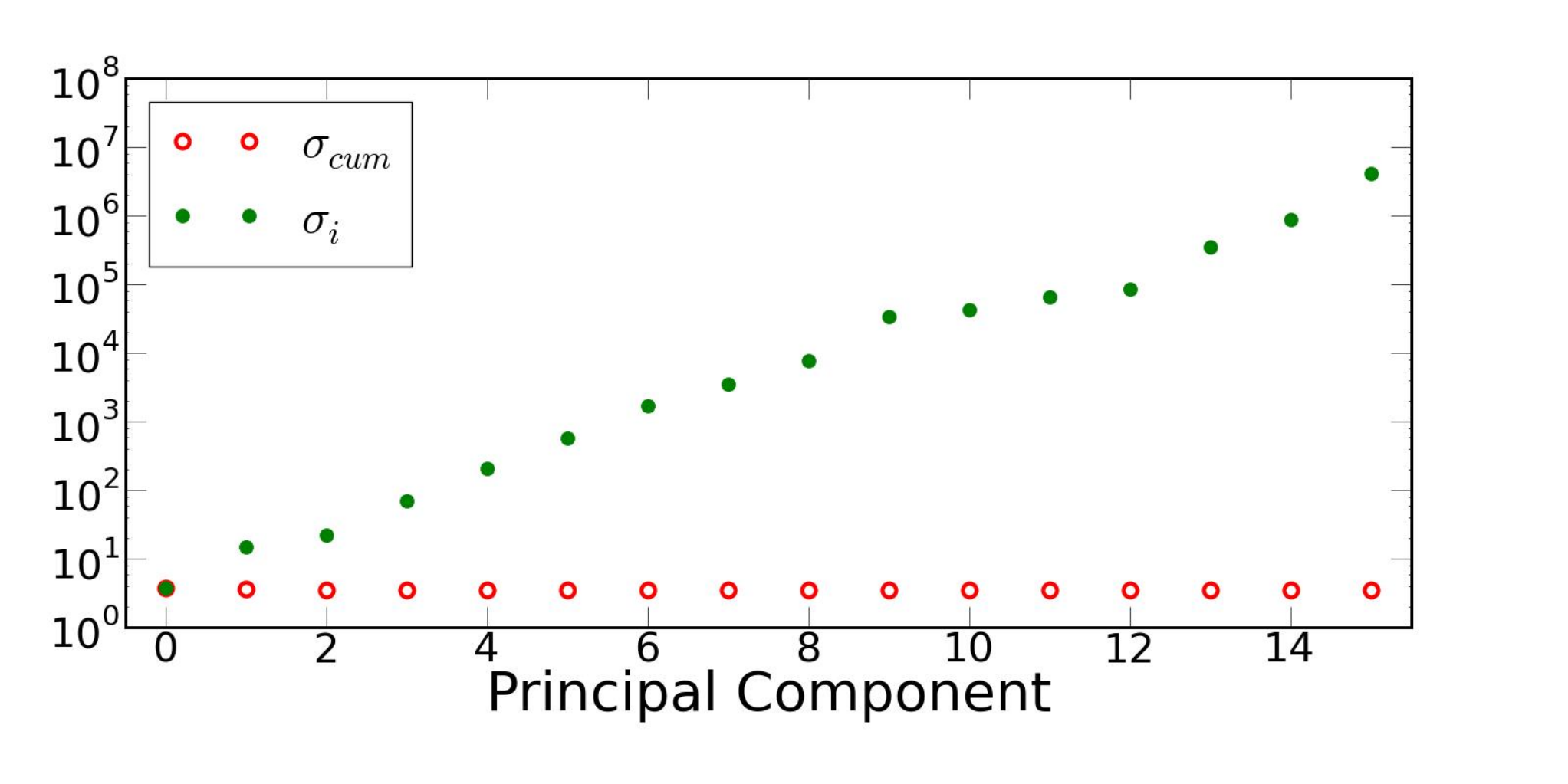
The error in the best-measured PC is 4.8; however, the error in the next-best measured PCs are 18.3 and 27.4, and the accuracy rapidly drops off from there. Thus, the first three or four PCs should be enough for any conceivable application. The error in each PC is plotted on a logarithmic scale in figure 4, along with the cumulative error $\sigma_{\rm cum}$, which is defined as

Each PC $e^{(j)}(k)$ has its own associated bispectrum (see Eq. (7)):

(As always, $k_{1},k_{2},$ and $k_{3}$ have a triangle relation: $k_{3}=|\vec{k_{2}}-\vec{k_{1}}|$.) We would like to test the similarity of these bispectra to those that have already been discussed in the literature. We can do this by using a distance measure between bispectra, defined by ‘cosines’ developed in [40]. A cosine near unity implies that the two bispectra have very similar shapes, and a cosine near zero implies the opposite. The cosine is defined as

where the inner product between two bispectra, $B_{1}\cdot B_{2}$, is [23]

The (Gaussian) variance of the bispectrum is

where $N_{T}$ is the number of distinct triangular configurations of $k_{1,2,3}$, and $P(k)\sim k^{-3}$ is the primordial curvature perturbation power spectrum. (The overall constant is irrelevant, since it cancels out in Eq. (39).)

We first compare our bispectra Eq. (38) to the local model with a constant $f_{\rm NL}$, whose bispectrum is (see Eqs. (1) and (17))

Most of the power of $B_{\rm local}$ is in so-called “squeezed” triangles, in which one side is much smaller than the other two (comparable) sides, $k_{1}<<k_{2}\approx k_{3}$.

Another form for the bispectrum much discussed in the literature is the “equilateral” bispectrum

In contrast with $B_{\rm local}$, most of the power of $B_{\rm equi}$ is in triangles where $k_{1}\approx k_{2}\approx k_{3}$; hence the name “equilateral”.

Table 1 lists the cosines of the first few principal-component derived bispectra with the local bispectrum and the equilateral bispectrum. The form of Eq. (38) suggests that the PC-derived bispectra $B^{(j)}$ will have more in common with the local bispectrum than the equilateral one. However, it is initially conceivable that some $e^{(j)}(k)$ might exist which would yield a bispectrum of the form in Eq. (43) when substituted into Eq. (38) – but in Appendix C, we prove that no such function exists. Thus, the only guarantees for the cosines of the $B^{(j)}$ are that the cosine of $B^{(0)}$ – the bispectrum corresponding to the best-measured PC – will be large with the local model, and that none of the $B^{(j)}$ have a very large cosine with the equilateral model. We expect the former because our model looks like the local model; we expect the latter because of the proof in Appendix C. Table 1 bears out this expectation. The small cosines with the equilateral form of non-Gaussianity are also unsurprising because equilateral non-Gaussianity is expected to have a strongly suppressed signal in the non-Gaussian halo bias [57].

References

- [1] J. Maldacena, Non-gaussian features of primordial fluctuations in single field inflationary models, Journal of High Energy Physics 5 (2003) 13, [arXiv:astro-ph/0210603].
- [2] V. Acquaviva, N. Bartolo, S. Matarrese, and A. Riotto, Second-order cosmological perturbations from inflation, Nucl. Phys. B667 (2003) 119–148, [astro-ph/0209156].
- [3] P. Creminelli, On non-gaussianities in single-field inflation, JCAP 10 (2003) 003, [astro-ph/0306122].
- [4] D. H. Lyth and Y. Rodriguez, The inflationary prediction for primordial non- gaussianity, Phys. Rev. Lett. 95 (2005) 121302, [astro-ph/0504045].
- [5] D. Seery and J. E. Lidsey, Primordial non-gaussianities in single field inflation, JCAP 06 (2005) 003, [astro-ph/0503692].
- [6] X. Chen, Primordial Non-Gaussianities from Inflation Models, Adv. Astron. 2010 (2010) 638979, [arXiv:1002.1416].
- [7] E. Komatsu, Hunting for Primordial Non-Gaussianity in the Cosmic Microwave Background, Class. Quant. Grav. 27 (2010) 124010, [arXiv:1003.6097].
- [8] E. Komatsu and D. N. Spergel, Acoustic signatures in the primary microwave background bispectrum, Phys. Rev. D 63 (Mar., 2001) 063002, [arXiv:astro-ph/0005036].
- [9] L. Verde, L.-M. Wang, A. Heavens, and M. Kamionkowski, Large-scale structure, the cosmic microwave background, and primordial non-gaussianity, Mon. Not. Roy. Astron. Soc. 313 (2000) L141–L147, [astro-ph/9906301].
- [10] R. Scoccimarro, E. Sefusatti, and M. Zaldarriaga, Probing primordial non-gaussianity with large-scale structure, Phys. Rev. D 69 (2004) 103513, [astro-ph/0312286].
- [11] D. Salopek and J. Bond, Nonlinear evolution of long wavelength metric fluctuations in inflationary models, Phys.Rev. D 42 (1990) 3936–3962.
- [12] T. Falk, R. Rangarajan, and M. Srednicki, The angular dependence of the three point correlation function of the cosmic microwave background radiation as predicted by inflationary cosmologies, Astrophys. J. 403 (1993) L1, [astro-ph/9208001].
- [13] X.-c. Luo and D. N. Schramm, Testing for the gaussian nature of cosmological density perturbations through the three-point temperature correlation function, Phys. Rev. Lett. 71 (1993) 1124–1127, [astro-ph/9305009].
- [14] A. Gangui, F. Lucchin, S. Matarrese, and S. Mollerach, The three point correlation function of the cosmic microwave background in inflationary models, Astrophys. J. 430 (1994) 447–457, [astro-ph/9312033].
- [15] L.-M. Wang and M. Kamionkowski, The cosmic microwave background bispectrum and inflation, Phys. Rev. D 61 (2000) 063504, [astro-ph/9907431].
- [16] N. Bartolo, E. Komatsu, S. Matarrese, and A. Riotto, Non-gaussianity from inflation: Theory and observations, Phys. Rept. 402 (2004) 103–266, [astro-ph/0406398].
- [17] D. Seery and J. E. Lidsey, Primordial non-Gaussianities from multiple-field inflation, JCAP 0509 (2005) 011, [astro-ph/0506056].
- [18] X. Chen, Running Non-Gaussianities in DBI Inflation, Phys. Rev. D 72 (2005) 123518, [astro-ph/0507053].
- [19] M. Liguori, F. K. Hansen, E. Komatsu, S. Matarrese, and A. Riotto, Testing primordial non-Gaussianity in CMB anisotropies, Phys. Rev. D 73 (Feb., 2006) 043505, [arXiv:astro-ph/0509098].
- [20] X. Chen, R. Easther, and E. A. Lim, Large non-Gaussianities in single field inflation, JCAP 06 (2007) 023, [astro-ph/0611645].
- [21] M. LoVerde, A. Miller, S. Shandera, and L. Verde, Effects of Scale-Dependent Non-Gaussianity on Cosmological Structures, JCAP 04 (2008) 014, [arXiv:0711.4126].
- [22] X. Chen, R. Easther, and E. A. Lim, Generation and Characterization of Large Non-Gaussianities in Single Field Inflation, JCAP 04 (2008) 010, [arXiv:0801.3295].
- [23] E. Sefusatti, M. Liguori, A. P. S. Yadav, M. G. Jackson, and E. Pajer, Constraining running non-gaussianity, JCAP 12 (Dec., 2009) 22, [arXiv:0906.0232].
- [24] J. Kumar, L. Leblond, and A. Rajaraman, Scale dependent local non-gaussianity from loops, JCAP 04 (Apr., 2010) 24, [arXiv:0909.2040].
- [25] C. T. Byrnes, S. Nurmi, G. Tasinato, and D. Wands, Scale dependence of local , JCAP 02 (Feb., 2010) 34, [arXiv:0911.2780].
- [26] C. T. Byrnes and K.-Y. Choi, Review of local non-Gaussianity from multi-field inflation, Adv. Astron. 2010 (2010) 724525, [arXiv:1002.3110].
- [27] D. Wands, Local non-Gaussianity from inflation, Class.Quant.Grav. 27 (2010) 124002, [arXiv:1004.0818].
- [28] A. Riotto and M. S. Sloth, Strongly Scale-dependent Non-Gaussianity, arXiv:1009.3020.
- [29] Q.-G. Huang, Scale dependence of in N-flation, arXiv:1009.3326.
- [30] S. Mollerach, Isocurvature Baryon Perturbations and Inflation, Phys.Rev. D 42 (1990) 313–325.
- [31] A. D. Linde and V. F. Mukhanov, Nongaussian isocurvature perturbations from inflation, Phys.Rev. D 56 (1997) 535–539, [astro-ph/9610219].
- [32] K. Enqvist and M. S. Sloth, Adiabatic CMB perturbations in pre - big bang string cosmology, Nucl.Phys. B 626 (2002) 395–409, [hep-ph/0109214].
- [33] D. H. Lyth and D. Wands, Generating the curvature perturbation without an inflaton, Phys. Lett. B 524 (2002) 5–14, [hep-ph/0110002].
- [34] T. Moroi and T. Takahashi, Effects of cosmological moduli fields on cosmic microwave background, Phys.Lett. B 522 (2001) 215–221, [hep-ph/0110096].
- [35] L. Kofman, Probing string theory with modulated cosmological fluctuations, astro-ph/0303614.
- [36] M. Zaldarriaga, Non-Gaussianities in models with a varying inflaton decay rate, Phys.Rev. D69 (2004) 043508, [astro-ph/0306006].
- [37] C. T. Byrnes, M. Gerstenlauer, S. Nurmi, G. Tasinato, and D. Wands, Scale-dependent non-Gaussianity probes inflationary physics, JCAP 10 (2010) 004, [arXiv:1007.4277].
- [38] C. T. Byrnes, K. Enqvist, and T. Takahashi, Scale-dependence of Non-Gaussianity in the Curvaton Model, JCAP 09 (2010) 026, [arXiv:1007.5148].
- [39] Q.-G. Huang, Negative spectral index of in the axion-type curvaton model, JCAP 11 (2010) 026, [arXiv:1008.2641].
- [40] D. Babich, P. Creminelli, and M. Zaldarriaga, The shape of non-gaussianities, JCAP 08 (2004) 009, [astro-ph/0405356].
- [41] S. Shandera, N. Dalal, and D. Huterer, A generalized local ansatz and its effect on halo bias, arXiv:1010.3722.
- [42] N. Dalal, O. Dore, D. Huterer, and A. Shirokov, The imprints of primordial non-gaussianities on large- scale structure: scale dependent bias and abundance of virialized objects, Phys. Rev. D77 (2008) 123514, [arXiv:0710.4560].
- [43] N. Afshordi and A. J. Tolley, Primordial non-gaussianity, statistics of collapsed objects, and the Integrated Sachs-Wolfe effect, Phys. Rev. D78 (2008) 123507, [arXiv:0806.1046].
- [44] S. Matarrese and L. Verde, The effect of primordial non-Gaussianity on halo bias, Astrophys. J. 677 (2008) L77, [arXiv:0801.4826].
- [45] A. Slosar, C. Hirata, U. Seljak, S. Ho, and N. Padmanabhan, Constraints on local primordial non-Gaussianity from large scale structure, JCAP 08 (2008) 031, [arXiv:0805.3580].
- [46] F. Schmidt and M. Kamionkowski, Halo Clustering with Non-Local Non-Gaussianity, Phys. Rev. D 82 (2010) 103002, [arXiv:1008.0638].
- [47] P. McDonald, Primordial non-Gaussianity: large-scale structure signature in the perturbative bias model, Phys. Rev. D78 (2008) 123519, [arXiv:0806.1061].
- [48] A. Taruya, K. Koyama, and T. Matsubara, Signature of primordial non-Gaussianity on the matter power spectrum, Phys. Rev. D 78 (Dec., 2008) 123534, [arXiv:0808.4085].
- [49] T. Giannantonio and C. Porciani, Structure formation from non-Gaussian initial conditions: multivariate biasing, statistics, and comparison with N- body simulations, Phys. Rev. D81 (2010) 063530, [arXiv:0911.0017].
- [50] M. Grossi, K. Dolag, E. Branchini, S. Matarrese, and L. Moscardini, Evolution of Massive Haloes in non-Gaussian Scenarios, Mon. Not. Roy. Astron. Soc. 382 (July, 2007) 1261, [arXiv:0707.2516].
- [51] V. Desjacques, U. Seljak, and I. T. Iliev, Scale-dependent bias induced by local non-Gaussianity: a comparison to N-body simulations, MNRAS 396 (June, 2009) 85–96, [arXiv:0811.2748].
- [52] A. Pillepich, C. Porciani, and O. Hahn, Halo mass function and scale-dependent bias from N-body simulations with non-Gaussian initial conditions, MNRAS 402 (Feb., 2010) 191–206, [arXiv:0811.4176].
- [53] C. Carbone, L. Verde, and S. Matarrese, Non-Gaussian halo bias and future galaxy surveys, Astrophys. J. 684 (2008) L1–L4, [arXiv:0806.1950].
- [54] B. Sartoris et al., The potential of X-ray cluster surveys to constrain primordial non-Gaussianity, arXiv:1003.0841.
- [55] C. Cunha, D. Huterer, and O. Doré, Primordial non-gaussianity from the covariance of galaxy cluster counts, Phys. Rev. D 82 (Jul, 2010) 023004, [arXiv:1003.2416].
- [56] V. Desjacques and U. Seljak, Signature of primordial non-Gaussianity of -type in the mass function and bias of dark matter haloes, Phys. Rev. D81 (2010) 023006, [arXiv:0907.2257].
- [57] L. Verde and S. Matarrese, Detectability of the effect of Inflationary non- Gaussianity on halo bias, Astrophys. J. 706 (2009) L91–L95, [arXiv:0909.3224].
- [58] B. Grinstein and M. B. Wise, Nongaussian Fluctuations and the Correlations of Galaxies or Rich Clusters of Galaxies, Astrophys. J. 310 (1986) 19–22.
- [59] S. Matarrese, F. Lucchin, and S. A. Bonometto, A path-integral approach to large-scale matter distribution originated by non-Gaussian fluctuations, Astrophys. J. 310 (Nov., 1986) L21–L26.
- [60] H. A. Feldman, N. Kaiser, and J. A. Peacock, Power spectrum analysis of three-dimensional redshift surveys, Astrophys. J. 426 (1994) 23–37, [astro-ph/9304022].
- [61] M. Tegmark, Measuring cosmological parameters with galaxy surveys, Phys. Rev. Lett. 79 (1997), no. 20 3806–3809, [astro-ph/9706198].
- [62] H. Seo and D. J. Eisenstein, Probing Dark Energy with Baryonic Acoustic Oscillations from Future Large Galaxy Redshift Surveys, Astrophys. J. 598 (Dec., 2003) 720–740, [arXiv:astro-ph/0307460].
- [63] E. Komatsu et al., Seven-Year Wilkinson Microwave Anisotropy Probe (WMAP) Observations: Cosmological Interpretation, arXiv:1001.4538.
- [64] K. Abazajian, K. Kadota, and E. D. Stewart, Parameterizing the power spectrum: Beyond the truncated Taylor expansion, JCAP 0508 (2005) 008, [astro-ph/0507224].
- [65] D. Huterer and G. Starkman, Parameterization of dark-energy properties: A principal- component approach, Phys. Rev. Lett. 90 (2003) 031301, [astro-ph/0207517].
- [66] A. J. Albrecht et al., Findings of the Joint Dark Energy Mission Figure of Merit Science Working Group, arXiv:0901.0721.