Maximizing Sequence-Submodular Functions and its Application to Online Advertising
Abstract
Motivated by applications in online advertising, we consider a class of maximization problems where the objective is a function of the sequence of actions as well as the running duration of each action. For these problems, we introduce the concepts of sequence-submodularity and sequence-monotonicity which extend the notions of submodularity and monotonicity from functions defined over sets to functions defined over sequences. We establish that if the objective function is sequence-submodular and sequence-non-decreasing, then there exists a greedy algorithm that achieves of the optimal solution.
We apply our algorithm and analysis to two applications in online advertising: online ad allocation and query rewriting. We first show that both problems can be formulated as maximizing non-decreasing sequence-submodular functions. We then apply our framework to these two problems, leading to simple greedy approaches with guaranteed performances. In particular, for online ad allocation problem the performance of our algorithm is , which matches the best known existing performance, and for query rewriting problem the performance of our algorithm is which improves upon the best known existing performance in the literature.
1 Introduction
Search advertising continues to power the growth of online advertising. For instance, Google AdWord’s revenue accounts for most of its revenue, amounting to over twenty billion dollars in the first quarter of 2018.11 1 https://www.cnbc.com/2018/06/27/googles-adwords-and-doubleclick-have-been-rebranded-and-reorganized.html At the core of advertising for such search engines, there is a demand to allocate relevant ads to user queries. Advertisers bid on queries that are most likely to generate clicks and conversions for them, and ad allocators want relevant ads for their users to maximize revenue on their platforms. This problem can be cast as an online allocation problem where the search engine decides on the order of the ads to show for a sequence of arriving queries. The goal of the ad allocator is to maximize its revenue which is a function of the sequence of allocations.
This online allocation problem demands to develop computationally efficient solutions with guaranteed performances. In this regard, the greedy approach is a natural choice leading to simple implementations. In particular, the greedy algorithm has the advantage that it can be applied in a variety of settings where complete knowledge of the problem is not available or in online settings where the input is revealed gradually. For maximizing set-submodular functions Nemhauser et al. (1978), Nemhauser and Wolsey (1978), and Wolsey (1982) show that a greedy algorithm achieves of the optimal solution (subject to some constraints). However, the online ad allocation objective function is defined over sequences rather than sets for which the order of allocations matter. This raises the question of whether there exists natural extensions of set-submodular functions to functions defined over sequences. In this paper, we develop such a framework which enables us to obtain performance guarantees for greedy algorithms that are the same as non-decreasing submodular functions over sets. We apply our algorithm and analysis to two applications in online advertising, namely, online ad allocation and query rewriting and provide computationally efficient algorithms with guaranteed performances.
1.1 Contribution
The contribution of our work is twofold. First, we introduce a framework for solving a broad class of maximization problems where the objective function is defined over sequences. In particular, we introduce the notion of sequence-submodular functions which extends the notion of submodularity over sets to submodularity over sequences. We define sequence submodularity over both continuous and discrete sequences and carry out the analysis of these two cases separately. Our main results show that if the objective function is sequence-submodular, sequence-non-decreasing, and in the case of continuous sequences differentiable, then a greedy approach achieves of the optimal solution subject to a constraint on the maximum length of the sequence. In our algorithm, we solve a collection of local optimization problems and then form a global solution based on the solution of these local problems. Furthermore, we show that even if the local problems cannot be solved optimally (e.g., because of limited computational or time resources), our algorithm and analysis still provide a performance guarantee. In particular, if the solutions of the local optimization problems are at least times the optimal local solutions, then our algorithm achieves of the overall optimal solution.
Second, we present two applications of our framework to search advertising. In our first application, we show that online ad allocation problem can be formulated as maximizing a sequence-submodular function. We then apply our algorithm and analysis and obtain a greedy algorithm that achieves of the optimal revenue, where the bid to budget ratio is defined as the ratio of the maximum payment to minimum budget.22 2 We consider a general ad allocation problem in which the query distribution is unknown. Therefore, we cannot use LP rounding to solve this problem. In particular, if the bid to budget ratio is very small, then our algorithm achieves of the optimal revenue. This is the same as the one obtained in Goel and Mehta (2008), using a more involved analysis based on the techniques developed in Karp et al. (1990). In our second application, we consider query rewriting for online ad allocation which is a technique to improve the relevance of ad allocation. Again, we show that ad allocation with query rewriting can be formulated as maximizing a sequence-submodular function. We then apply our algorithm and analysis and obtain a greedy algorithm that achieves of the optimal solution. In particular, if the bid to budget ratio is very small, then our algorithm achieves of the optimal revenue, improving upon the approximation of Malekian et al. (2008).
1.2 Related Work
Submodularity has been studied in more depth in recent years because of its applications to combinatorial auctions and the fact that many important problems in computer science, economics, and operations can be formulated as submodular function maximization. Instances include submodular welfare maximization problems such as Lehmann et al. (2006), Khot et al. (2005), Dobzinski and Schapira (2006), Vondrák (2008), Feige (2009); viral marketing and influence maximization over a network such as Kempe et al. (2003), Mossel and Roch (2010); and generalized assignment problems such as Fleischer et al. (2006). Another prominent application is machine learning and in particular data summarization Mirzasoleiman et al. (2016), Lin and Bilmes (2011), recommender systems Gabillon et al. (2013), and crowd teaching Singla et al. (2014).
The greedy approach is a natural tool to solve maximization problems with a submodular objective function. Nemhauser and Wolsey (1978) show that the greedy approach gives a -approximation for maximizing a non-decreasing submodular function over a uniform matroid. Nemhauser et al. (1978) consider this problem over the independence system. They show that if the independence system is the intersection of matroids, the greedy algorithm gives a approximation. Goundan and Schulz (2007) generalize both of these results and show that if an -approximate incremental oracle is available, then the greedy solution is a approximation for maximizing a non-decreasing submodular function over a uniform matroid and an approximation for the intersection of matroids. Feige et al. (2011) provide a general framework for solving the non-monotone submodular problems. More recently, Asadpour and Nazerzadeh (2015) and Adamczyk et al. (2016) study maximizing stochastic submodular functions. In particular, Asadpour and Nazerzadeh (2015) show that a greedy algorithm obtains of the optimal value subject to a matroid constraint. Furthermore, they prove that the greedy algorithm obtains of the optimal value for uniform matroid constraints. Relatedly, Golovin and Krause (2011) extend submodularity to adaptive policies for solving stochastic optimization problems under partial observability.
Our paper generalizes the concept of submodularity to functions defined over sequences instead of sets. Since the circulation of an early version of our paper, extensions of submodularity to other interesting settings have been studied in Li and Milenkovic (2017), Tschiatschek et al. (2017), and Mitrovic et al. (2018). In particular, Li and Milenkovic (2017) consider a combination of submodularity and hypergraphs within the context of hypergraph clustering. More recently, Tschiatschek et al. (2017) and Mitrovic et al. (2018) use a directed graph connecting the items together with a submodular function on its edges to define functions over sequences. In their setting, the edges of the directed graph encode the additional value of selecting elements in a particular order. Their setting and results are different from ours. In particular, the sequence functions that are defined with directed graphs do not have diminishing return property and are not equivalent to our class of sequence-submodular functions. Moreover, the guarantee of their proposed algorithm depends on the maximum degree in the underlying graph and the length of the sequence and is worse than .
Our first application is online ad allocation problem. There is a considerable amount of work on AdWords auctions and in particular online ad allocation problem (see Mehta (2013) for a survey). In the online ad allocation problem, the goal is to match incoming queries to advertisers with the goal of maximizing the revenue. Several papers such as Mehta et al. (2007), Lahaie et al. (2007) have studied this problem. In particular, assuming that the maximum bid is very small compared to budgets, Mehta et al. (2007) provide a deterministic algorithm with the competitive ratio of in the worst case model. It can be shown that the competitive ratio for the greedy algorithm is in the worst case model. Subsequently, Goel and Mehta (2008) showed that the competitive ratio of the greedy approach in the i.i.d model is and the analysis is tight. Their proof is partly based on the techniques used in Karp et al. (1990) for the online bipartite matching problem. Our framework, however, provides a simple greedy algorithm that achieves the same competitive ratio (under the same common assumption that the maximum bid is very small compared to budgets). The offline variant of ad allocation has been studied in Andelman and Mansour (2004) and Fleischer et al. (2006), where they show that the problem is NP-complete with the best known approximation factor of .
Our second application is query rewriting in online ad allocation. There is a large literature on clustering and mining of search logs to generate query suggestions for improving web and paid search results. The goal of query rewriting is to define a succinct set of rewrites and assign each query to a subset of rewrites. With query rewriting, for each arriving query, the ad allocator finds the most relevant ad by searching over the ads associated with the rewrites assigned to that query (see Jones et al. (2006), Zhang and Jones (2007), and Singh et al. (2012)). In particular, Malekian et al. (2008), consider the problem of query rewriting in the context of search advertising and provide an algorithm that achieves of the optimal revenue. Again, our framework provides a simple greedy algorithm that achieves the improved approximation.
1.3 Organization
In Section 2, we formulate the online ad allocation problem as maximizing a function defined over continuous sequences. In Section 3, we introduce non-decreasing sequence-submodular functions over continuous sequences and establish that in maximizing such a function, a greedy algorithm achieves of its optimal solution. We then show that the objective function formulating the online ad allocation problem is non-decreasing and sequence-submodular, showing that a greedy algorithm achieves of its optimal solution. In Section 4, we introduce query rewriting problem in the context of search advertising and formulate it as maximizing a function defined over discrete sequences. In Section 5, we describe our framework for maximizing non-decreasing sequence-submodular functions defined over discrete sequences. We then show that the objective function formulating the query rewriting problem is non-decreasing and sequence-submodular, and establish that our greedy algorithm achieves of its optimal solution. We conclude the paper in Section 6. All the omitted proofs are included in the appendix.
2 Online Ad Allocation
Search advertising constitutes one of the largest resource allocation problems, both in terms of the capital and the number of items. In online advertising mechanisms used by search engines, advertisers submit their bid to the search engine for each keyword (also referred to as query type) and their total budget. Whenever a user searches for a service or product, the search engine (also referred to as ad allocator) decides on a set of relevant ads to display. At the core of this service, there is an allocation algorithm that allocates ads to an arriving query, based on the relevance of the query to ads and the budget of advertisers. This problem is inherently online since the ad allocator needs to show ads whenever a query arrives, and it does not have complete information about the arriving queries in advance. The objective of this online ad allocation problem is to find a way to perform this allocation to achieve maximum revenue. We next formally define this problem.
2.1 Problem Formulation
We let denote the set of ads (also referred to as advertisers), and denote the set of query types. When a query arrives, the ad allocator assigns this query to a set of ads to be displayed along-side organic results. To capture the limit on the number of slots for sponsored ads, we assume each query is assigned to at most ads. Each assignment of a query to an advertiser generates revenue for the ad allocator which is equal to the payment of the advertiser. In particular, we let be the payment of advertiser to the ad allocator for showing ad to a query of type . This payment is a function of the click-through rate of the ad, the relevance of the ad to the query, the bid of the advertiser for that query, and possibly other parameters. Each advertiser has a limited budget and showing the ad of an advertiser that has consumed her entire budget cannot provide revenue. For each advertiser , we let denote its budget which represents the total payment the advertiser is willing to pay for a given period of time. Therefore, at each time (based on the remaining budgets of the advertisers and the payments) the ad allocator should decide on the mapping from queries to ads, defined next.
Definition 1 (Configuration).
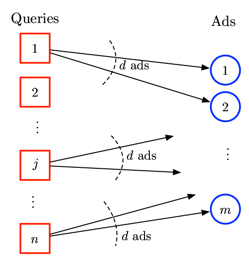
A configuration is a mapping from query types to ads such that each query type is mapped to at most ads. Formally, a configuration is a collection of sets for all such that . We let be the set of all possible configurations. Figure 1 illustrates the definition of configuration.
The revenue of the ad allocator is the sum of the revenues generated for each query given the configuration that is used by the ad allocator, as described next.
2.2 Ad allocator’s Decision and Revenue
We let denote the end of time horizon and assume a sequence of queries are arriving over according to a Poisson point process with rate (the rate one assumption has no bearing on our results, but simplifies the exposition). The type of each query is an i.i.d. random variable drawn from a fixed but possibly unknown distribution where is the probability of a query being of type . Therefore, for any interval of length , the expected number of type queries arriving in a period of length is .
The next definition captures the decision of ad allocator regarding the sequence of configurations used during the period .
Definition 2 (Allocation Strategy).
We call any sequence of configurations over time an allocation strategy which is represented by
where , , , and . This sequence indicates that the ad allocator uses each configuration (in order) for a duration of for all . We let denote the set of all possible allocation strategies.
For any given allocation strategy we let be the expected revenue of the ad allocator for using allocation strategy , where the expectation is taken with respect to the Poisson random process governing the arrival of queries and distribution for the type of queries. Therefore, the problem of the ad allocator can be written as
Note that the sequence can be chosen adaptively. That is, for any , the configuration used at time depends on the query types that have arrived before time as well as the configurations used to serve those queries.33 3 More precisely, if for any we let be the -algebra of the events happened in the interval , then the configuration used at time must be -measurable. In the next example, we illustrate the definition of allocation strategy and revenue of the ad allocator.
Example 1.
Suppose and there are two advertisers and two query types, i.e., and . We let and the payments be
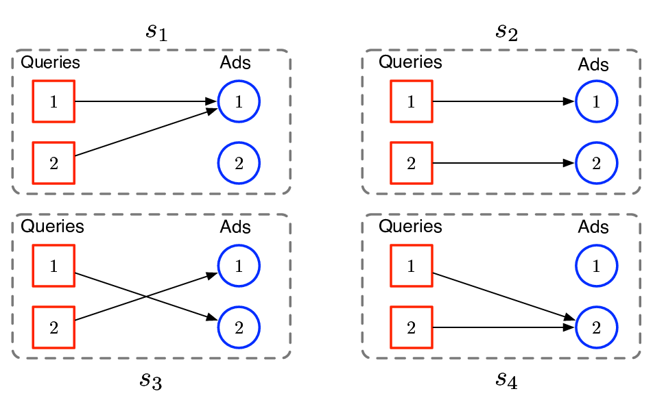
and the budgets be and . We also let and be the probability of query types and , respectively. In this setting, there exist four possible configurations as follows (see Figure 2)
For instance, configuration maps both queries to ad and configuration maps queries of type to ad and queries of type to ad . We next find the revenue of the allocation strategy , i.e., running configuration for duration . Since , for both types of queries the ad allocator shows ad until ad runs out of budget. We let be the number of type one queries in period and be the number of type two queries. For a given and , to find the revenue we need to consider the following cases:
- •
The budget constraint is not binding, i.e., : in this case, we can show ad for both types of queries for the entire time interval. The generated revenue in this case becomes .
- •
The budget constraint is binding, i.e., : in this case we can only show ad so long as its remaining budget is above the payment for the query type. In this case, the revenue belong to the interval .
3 Continuous Sequence-Submodular Functions and their Maximization
In this section, we define our framework for sequence submodular function maximization and then apply it to online ad-allocation problem. To this end, we first introduce continuous sequences together with the notion of sequence functions, their monotonicity, and their submodularity. We then find a greedy algorithm to maximize sequence submodular functions and establish its performance. Finally, we apply our algorithm and analysis to online ad allocation problem.
3.1 Continuous Sequences: Definition and Operations
For any finite set of elements , the sequence where and and is called a continuous sequence. The length of a continuous sequence denoted by is equal to . We denote the set of all finite continuous sequences of by , formally defined as
Throughout, we use to denote the empty sequence. For instance, each allocation strategy in online ad allocation problem is a continuous sequence where each configuration (see Definition 1) is an element and each allocation strategy (see Definition 2) is a continuous sequence.
We say two continuous sequences and are equivalent and denote it by if they have the same length and their corresponding elements are the same. We next define three key operations on continuous sequences which we use throughout our analysis.
Definition 3 (Concatenation).
For two continuous sequences and , their concatenation denoted by is a new sequence that is the result of attaching the beginning of sequence to the end of sequence .
For instance, in the context of online ad allocation the concatenation of two allocation strategies and , i.e., is an allocation strategy that uses the configurations specified by (in order) followed by configurations specified by .
Definition 4 (Refinement).
The refinement of a continuous sequence in the interval denoted by is a subsequence of that contains all the elements of starting from time to time . Formally, we have
where and are uniquely defined from the following relations:
For instance, in the context of online ad allocation, the refinement of allocation strategy in the interval is an allocation strategy which contains all the configurations specified by (in the same order) from time to time .
Definition 5 (Domination).
A continuous sequence is dominated by another continuous sequence , denoted by , if we can remove some elements of to obtain . Formally, for two continuous sequences and , we have if and only if there exists and such that
For instance, in the context of online ad allocation for two allocation strategies and we have , if we can obtain be removing some of the configurations in (by either decreasing their running time or eliminating the configuration entirely) and keeping the order of the remaining configurations.
In the next section, we use these three operations to define the class of submodular non-decreasing continuous sequence functions.
3.2 Submodular Non-decreasing Continuous Sequence Functions
Continuous sequence functions are functions whose domain are continuous sequences. Formally, given a finite set , any function is a continuous sequence function. We next define the key attributes of continuous sequence functions, namely sequence-non-decreasing, sequence-submodularity, and differentiability. These attributes are the analogy of non-decreasing submodular functions defined over sets and enable us to provide performance guarantees for greedy algorithms in maximizing continuous sequence functions.
Definition 6.
A continuous sequence function is sequence-non-decreasing if
| (1) |
A continuous sequence function is sequence-submodular if
| (2) |
where is the marginal value of the sequence function defined as
A continuous sequence function is differentiable if for any , is continuous and differentiable with a continuous derivative with respect to for all except at a finite number of points for which it may have different left and right derivatives and hence a non-continuous derivative.
In the next section, we provide a greedy algorithm to maximize any continuous sequence function satisfying the following assumption.
Assumption 1.
The continuous sequence function is sequence-non-decreasing, sequence-submodular, and differentiable.
3.3 Greedy Algorithm for Maximizing Continuous Sequence Functions
In this section, we consider the problem of maximizing a continuous sequence function subject to a given length constraint. In particular, we develop a greedy algorithm for such maximization problem and establish its performance guarantee for sequence functions satisfying Assumption 1.
For a given and continuous sequence function , and time horizon , the objective is to find a sequence that maximizes subject to the length constraint , i.e.,
| s.t. | (3) |
We next introduce a notation that we use in stating our algorithm and results for the continuous setting. For an element , time duration , and continuous sequence , we define as
| (4) |
which represents the rate of increasing if we continue using element after using it for duration . We also define
| (5) |
which represents the rate of increasing if we start using element after using sequence . Note that is always defined (except for finite number of points) because (4) can be rewritten as follows
and by Assumption 1 (in particular, differentiability) exists except for a finite number of points. Also note that with Assumption 1, is a continuous function over except at a finite number of points.
Our key result presented next establishes the performance of a greedy algorithm for maximizing continuous sequence functions.
Theorem 1.
Theorem 1 states that if the elements of the sequence are chosen such that at each point , the derivative of is at least times its optimal local maximum, then the resulting sequence yields of the optimal solution (global maximum).
We next outline the key idea of this result for (the complete proof is given in the Appendix). First, using sequence-submodularity and differentiability, we show that the rate of increase in the function value with the greedy choice is as large as the time average marginal increase by concatenating any other sequence. Formally, for all and we show
Substituting the optimal sequence, i.e., , for and then using non-decreasing property, we show that this rate of increase is as large as the time average difference between the function value of the optimal solution and the function value of the current sequence. Formally, we have
This provides a recursive relation between the utility of the greedy choice and the optimal choice. Using this recursive relation we then establish that the function value of sequence is at least times the function value of the optimal solution .
Motivated by Theorem 1, Algorithm 1 presents our greedy algorithm for maximizing non-decreasing, submodular, and differentiable sequence functions.
Algorithm 1 starts with an empty sequence (the initialization is ) and at each time finds an element together with an interval of running it (i.e., ) such that at any time in this interval, the rate of increasing function is at least times the maximum rate of increase among all elements of . The following which is an immediate corollary of Theorem 1 formally states the performance of Algorithm 1.
Corollary 1.
We point out a few remarks regarding Algorithm 1. First, note that the algorithm, in general, may not terminate, however, if it terminates with the resulting , then is at least times the optimal solution. Second, in Algorithm 1, each time that we switch the element in use, we need an incremental oracle to find the next element and the duration of using it which is -optimal. This incremental oracle is specific to each problem. We next show that for online ad allocation problem, the algorithm terminates in finite time and the incremental oracle can be found exactly, i.e., with .
3.4 Application to Online Ad Allocation
We first introduce a slight variation of the online ad allocation problem and then show the revenue function for that variation satisfies Assumption 1. We then use Theorem 1 to establish the performance of our greedy algorithm for the variation. Finally, using these results, we establish the performance of the greedy algorithm for the original online ad allocation problem.
Recall that is the payment of advertiser to the ad allocator for showing ad to a query of type . Also, the type of each query is an i.i.d. random variable drawn from a fixed but possibly unknown distribution where is the probability of a query being of type . Also, recall that is the set of configurations for online ad allocation problem, is the set of all allocation strategies, and is a function that maps an allocation strategy to its expected utility.
We consider a variation of online ad allocation problem in which whenever an advertiser runs out of budget (i.e., its budget is less than the payment of the ad specified by the configuration in use) the ad allocator shows the ad for a fraction of time and charges the advertiser for that fraction. We let be the function that maps an allocation strategy to its expected utility in this variation of online ad allocation problem.
In the next lemma we show that the utility function of the variation of online ad allocation problem satisfies Assumption 1.
Lemma 1.
The expected revenue of the variation of online ad allocation problem , i.e., is sequence-non-decreasing, sequence-submodular, and differentiable.
We next outline the idea to prove sequence-submodularity of the variation of online ad allocation problem (the complete proof of all properties is given in the appendix). We next consider the allocation strategies with and show . The idea is to compare the contribution of each ad to and . We first show that the remaining budget of each advertiser after is greater than (or equal to) its budget after running . We then divide ads into two categories:
- •
Ads that have exhausted all of their budget after running . The contribution of these ads to is all their remaining budgets after running . On the other hand, the contribution of these ads to is at most their remaining budget after running , which is smaller than their contribution to .
- •
Ads that still have budget after running . Since these ads do not run out of budget, the allocation strategy (when running after ) has extracted revenue from these ads at the full rate.
Lemma 1 together with Theorem 1 establish the performance guarantee of an allocation strategy obtained by using greedy algorithm for the variation of the online ad allocation problem. Using this result, we next show the performance guarantee of an allocation strategy obtained by using greedy algorithm for the original online ad allocation problem.
Lemma 2.
Let be the allocation strategy obtained by running greedy algorithm for the original online ad allocation problem. We have
where is the optimal allocation strategy.
This lemma establishes the performance guarantee of an allocation strategy obtained by running Algorithm 1, i.e., by greedily choosing the configuration with the highest rate of revenue increase (equivalently, finding such that Eq. (6) holds with ). To find such a configuration, we need to compute , which we find in the next lemma.
Lemma 3.
Let be the set of configurations for online ad-allocation problem and let be an allocation strategy. For any and , we have
assuming that all ads specified by have budget.
This lemma holds because for a Poisson point process with rate as the probability of having more than one query in an interval of length is and the probability of having one query is . Therefore, as , becomes the expected revenue generated by one arriving query. Since the arriving query is of type with probability , the expected increase in the revenue becomes .
Using Lemma 3, if at time the ad allocator uses configuration such that for all
| (7) |
where is the set of ads which still have budget, then we have
Also note that we can keep using a configuration until at least one of the ads runs out of budget. We then update the set to become the set of ads which still have budget and recompute the best configuration as given in Eq. (7). The complete specification of Algorithm 1 to online ad allocation problem is given in Algorithm 2.
Note that this algorithm does not require the knowledge of the distribution . This is because as shown in Eq. (7), we can find the best configuration without knowing . The following proposition formally states the performance of Algorithm 2 for solving online ad allocation problem.
Theorem 2.
Greedy Algorithm 2 finds an allocation strategy whose expected revenue is at least
of the optimal expected revenue.
Theorem 2 directly follows from Lemmas 1, 2, and 3 and establishes the performance guarantee of our algorithm which holds for any bid to budget ratio. As a corollary of this proposition, if the bid to budget ratio is very small, then our algorithm achieves of the optimal solution. This approximation factor is also shown by Goel and Mehta (2008) using an involved analysis based on the techniques of Karp et al. (1990), under the same assumption that the bid to budget ratio is very small.
4 Query Rewriting
In search advertising, advertisers bid on queries that are most likely to generate clicks and conversions for them. Ad allocators then match advertisers to user queries that are relevant to the advertisers. However, one issue is that a relevant ad for a given query may not necessarily exist among the set of ads that have bid for that query. Indeed, that set may be empty even though a relevant ad exists. For instance, an ad bidding on the keyword “wedding band” may be appropriate for the query “engagement ring”. Another issue is that the advertiser bidding strategy for queries is ever-changing. Indeed, advertisers manage their budget throughout a given period by turning on and off their ads (either automatically or manually). This demands a system that can swiftly adapt to these changes by recomputing the keyword-ad relevance (e.g., with a machine-learned relevance ranking model), incorporating the changes in the availability of advertisers. Therefore, it is more practical to associate queries to a few keywords and then add (or remove) the list of advertisers of those keywords (the ones they are bidding on) rather than hundreds or even thousands of queries.
To address these issues, a common mechanism for search engines is query rewriting. At the high level, query rewriting outputs a list of keywords, referred to as rewrites, that are relevant for queries in the original list.
4.1 Problem Formulation
In query rewriting, the search engine associates each query with a set of rewrites. When a query arrives, the ad allocator assigns this query to a set of ads that have bid for at least one of the rewrites associated with that query. Therefore, the query rewriting problem becomes an online ad allocation problem with the constraint that only ads that have bid on the relevant rewrites to an incoming query can be displayed.
Formally, we denote the set of rewrites with . Each rewrite is relevant for a subset of advertisers, i.e., only the subset of advertisers bidding on rewrite , denoted by . The search engine associates each query type with a subset of rewrites denoted by . For an incoming query of type , the ad allocator decides on ads from the set to display. For instance, the query “engagement ring” can be associated with rewrite “wedding band”. Now if the advertisers in “wedding industry” have bid on “wedding band”, their ad can be shown for the query “engagement ring”. Note that too many rewrites for a given query will slow down the time needed to serve an ad. To address this issue, we restrict the set of associated rewrites with each query type to have at most rewrites, i.e., for all . Therefore, the query rewriting problem is how to find a set for all such that together with the corresponding allocation strategy to maximize the revenue of the ad allocator.
We suppose that in the time interval there are incoming queries of type , where is known. The order of the incoming queries, however, is unknown and random. This is a common assumption in practice because search engines have access to historical data and can estimate the distribution of the queries. It is also the same assumption as the one used in Malekian et al. (2008) and Mehta (2013).
Similar to the online ad allocation problem, given the set of rewrites, at each time the ad allocator should decide on the mapping from queries to ads, defined next.
Definition 7 (Query Rewriting Configuration).
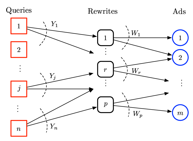
For a given , denoting the set of rewrites associated with each query, a query rewriting configuration, denoted by , maps a given query to at most ads among those included in the set of rewrites associated with query . Formally, is a collection of sets such that for all (see Figure 3 for an illustration of a query rewriting configuration). We let be the set of all such configurations. For a given sequence of queries and configurations the revenue of the ad allocator is the sum of the revenues generated for each query. We can represent the allocation of ads to queries over time by a sequence
This sequence indicates that the ad allocator uses configuration for the th query. We call a query rewriting allocation strategy and let denote the set of all such strategies.
We also let denote the expected revenue of the ad allocator for using strategy where the expectation is taken over all possible permutations of queries of type for all . The query rewriting problem is to choose the set of rewrites (before the queries arrive) together with a query rewriting allocation strategy to maximize , i.e.,
| (8) | ||||
| s.t. |
Note that the sequence can be chosen in an adaptive way. In particular, the th configuration (i.e., ) can depend on the query types that have arrived before time as well as the configurations used to serve those queries (i.e., ). However, the set of rewrites are chosen in an offline fashion before the allocation of ads to queries start.
To specify a query rewriting allocation strategy , we need to specify the configuration used at any time. We next define a discrete sequence which provides a compact representation of the query rewriting allocation strategy. Any query rewriting allocation strategy to serve a sequence of arriving queries determines the consumed budget that each advertiser allocates to each query type. We let be the expected consumed budget of advertiser in serving query type . We also let be the vector of budgets the ad allocator extracts in displaying ad for query type during . Therefore, each query rewriting allocation strategy determines the tuples where is a query type and is the set of rewrites for query type .
We next provide an alternative formulation of query rewriting problem. To simplify the exposition, we introduce this alternative formulation for . All the results continue to hold for any general as we show in Appendix 7.2.
Definition 8 (Partial Configuration and Compact Allocation Strategy).
We call the tuple a partial configuration, where is a query type, such that is the set of rewrites for query type , and is a vector of budgets in which is the maximum budget that we allow the ad allocator to extract in displaying ad for query type . We let be the set of all partial configurations. We call a discrete sequence from the elements of a compact allocation strategy, which is of the form
where is a permutation of . denotes the set of all compact allocation strategies.
For any compact allocation strategy , its revenue function denoted by is the revenue collected by sequentially running the partial configurations specified by sequence and extract the optimal revenue given the budget constraints. The budget constraints are imposed by both the remaining budget of the advertisers and the budget vector of the current partial configuration. We next formally define the revenue function of a compact allocation strategy.
Definition 9.
[Revenue Function of Compact Allocation Strategy] For a given compact allocation strategy we recursively define its revenue function. We let be zero and initialize the current budget of advertiser denoted by as the original budget of advertiser , i.e., . Suppose is the current element of (with the order specified by ). The budget limit of advertiser is the minimum of the current budget and . For queries of type , considering the remaining budget limits and the given rewrite set , we greedily select the optimal query rewriting configuration. That is for the first query of type we use configuration such that
where the advertisers without budget are deleted from the set . We then use this configuration until we meet the budget constraint of advertiser . We then update the configuration and switch to the ad with the second highest payment. We continue this approach for all queries of type . We also assume whenever an advertiser runs out of budget (i.e., its budget is less than the payment of the ad specified by the configuration in use) the ad allocator shows the ad for a fraction of time and charges the advertiser for that fraction. We add the collected payments to the current and update by subtracting the consumed budget of advertiser in serving query type . We then proceed to the partial configuration in the sequence and the revenue function is the revenue obtained at the end of this procedure.
Note that any compact allocation strategy defines a query rewriting allocation strategy in which for any arriving query the ad allocator uses the configuration specified in computing revenue function of compact allocation strategy (Definition 9). Moreover, for any query rewriting allocation strategy, the revenue obtained from its corresponding compact allocation strategy (where the query types are ordered in an arbitrary order in the sequence) is exactly the same as the revenue from the query rewriting allocation strategy itself. This is because for all query types the ad allocator shows each ad with the same frequency in both allocation strategies (potentially in a different order though).55 5 Note that since the budget consumed by all query types in the query rewriting allocation strategy is at most the advertiser’s budget, in the compact allocation strategy any order of query types obtains the same revenue as the original query allocation strategy. However, for a general compact allocation strategy, different orders of the query types in the discrete sequence generates different amount of revenue (when the advertiser budgets become binding).
Using this alternative formulation, the query rewriting problem (8) is equivalent to find together with a compact allocation strategy that maximizes , i.e.,
| (9) | ||||
| s.t. |
In the next section, we provide an algorithm for maximizing discrete sequence functions and then use it to find the optimal compact allocation strategy (i.e., to solve (9)).
5 Discrete Sequence-Submodular Functions and their Maximization
In this section, we define our framework for maximizing discrete sequence submodular functions and then apply it to query rewriting problem.
5.1 Discrete Sequences: Definition and Operations
We let be a finite set of actions. Any sequence where and is called a discrete sequence of elements of (with convention, for we have an empty sequence). The length of a discrete sequence denoted by is equal to . We again denote the set of all finite discrete sequences of by , formally defined as
Equivalency, concatenation and domination are similar to the continuous setting described in Section 3. The refinement of a discrete sequence in the set denoted by is . To be consistent with the continuous setting, we represent the set by .
5.2 Submodular Non-decreasing Discrete Sequence Functions
In this subsection, we define the class of submodular non-decreasing discrete sequence functions. Given a finite set , any function is a discrete sequence function.
Similar to the continuous setting, a discrete sequence function is sequence-non-decreasing if
| (10) |
Also, a discrete sequence function is sequence-submodular if
| (11) |
where is the marginal value of the sequence function defined as
In the next section, we provide a greedy algorithm to maximize any discrete sequence function satisfying the following assumption.
Assumption 2.
The discrete sequence function is sequence-non-decreasing and sequence-submodular.
5.3 Greedy Algorithm for Maximizing Discrete Sequence Functions
For a given , a discrete sequence function , and a length constraint , the objective is to find a sequence that maximizes subject to , i.e.,
| s.t. | (12) |
Our key result presented next establishes the performance guarantee of a greedy algorithm for maximizing discrete sequence functions.
Theorem 3.
Suppose Assumption 2 holds for a discrete sequence function . For any and a sequence in , if for all we have
| (13) |
then
| (14) |
where denotes the optimal solution of problem (12).66 6 The optimal solution exists because there are finitely many sequences of length at most . In particular, there are no more than many sequences with , where denotes the cardinality of set .
Theorem 3 shows that if the elements of the sequence are chosen sequentially such that for each , is at least times its optimal local maximum, then the resulting sequence yields of the optimal sequence.
We next outline the key idea of this result for (the complete proof is given in the Appendix). First, using sequence-submodularity, we show that the marginal increase in function value with the greedy choice is as large as the time average marginal increase by concatenating any other sequence. Formally, for all and we show
Substituting the optimal sequence, i.e., , for and then using non-decreasing property, we show that this marginal increase is as large as the time average difference between function value of the optimal solution and function value of the current sequence. Formally, we have
This provides a recursive relation between the function value of the greedy choice and the optimal choice. Using this recursive relation we then establish that the utility of sequence is at least fraction of the function value of the optimal solution .
Motivated by Theorem 3, Algorithm 3 presents our greedy algorithm for maximizing discrete sequence functions satisfying Assumption 2.
Algorithm 3 starts with an empty sequence (the initialization is ) and at each step adds one element to the sequence. For instance with , at step the algorithm finds that generates the highest increase in the value of when concatenated to the end of the current sequence (i.e., finds that maximizes ). Also note that in Algorithm 3, at step the problem of finding that maximizes may be computationally hard. Theorem 3 states that even if is times the local maximum, Algorithm 3 still provides a good approximation of the optimal solution, namely approximation. For instance, in Subsection 5.4, we show that for query rewriting, the local problem at each step can efficiently be solved with .
The following is an immediate corollary of Theorem 3 and formally states the performance of Algorithm 3.
Corollary 2.
5.4 Application to Query Rewriting
We first show that the revenue function of compact allocation strategy is non-decreasing and sequence-submodular. We then show that the local optimization problems of the greedy algorithm can be solved with . Finally, we use our analysis of Subsection 5.3, which finds a greedy algorithm for the compact allocation strategy (and equivalently, query rewriting problem) that achieves of the optimal revenue.
We start by showing the function satisfies Assumption 2.
Lemma 4.
The revenue function of compact allocation strategies, i.e., is sequence-non-decreasing and sequence-submodular.
The proof of this lemma is similar to that of Lemma 1 and is given in the appendix.
We next describe a greedy algorithm for maximizing and then use Theorem 3 to establish its performance. The greedy algorithm works as follows. At each step of the algorithm with the current allocation and current budget vector , for any remaining query type such as we greedily find the optimal set of rewrites with cardinality constraint . We then greedily select the tuple whose addition to the current strategy increases the revenue the most. Finally, we update the advertisers’ budgets by subtracting and update by appending to it. The complete algorithm is described in Algorithm 4.
Our next lemma establishes the performance of Algorithm 4.
Lemma 5.
Algorithm 4 finds a compact allocation strategy whose revenue function is at least of the optimal compact allocation strategy.
This lemma follows from applying Algorithm 3 to maximize and then using Theorem 3 with . In particular, in the local optimization step of Algorithm 3, we greedily find a set of rewrites subject to a cardinality constraint. We show that the greedy approach solves the local optimization problem with . The result then follows from using Lemma 4 and Theorem 3. The complete proof is given in the appendix.
The output of Algorithm 4 naturally defines a query rewriting allocation strategy as follows. For all , we let be the set of rewrites found by Algorithm 4. For arriving queries of type , we use the query configurations specified in computing of the output of Algorithm 4. We next find the performance guarantee of this query rewriting allocation strategy.
Theorem 4.
The query rewriting allocation strategy defined based on the output of Algorithm 4 achieves
of the optimal query rewriting allocation strategy.
Theorem 4 follows from Lemmas 4 and 5 and establishes the performance guarantee of our algorithm which holds for any bid to budget ratio. We next make a few remarks regarding Algorithm 4 and its corresponding query rewriting allocation strategy. First, note that this algorithm requires the knowledge of the distribution (same as the algorithm of Malekian et al. (2008)). This is because in defining the function we need to know the number of queries of type in the time interval . The order of incoming queries, however, is unknown and random. Second, using Theorem 4 for small bid to budget ratio, the query rewriting allocation strategy defined based on the output of Algorithm 4 achieves . This outperforms the existing algorithm with approximation factor given in Malekian et al. (2008).
6 Conclusion
Motivated by applications in online advertising, we develop a framework to maximize functions defined over sequences. In particular, we extend the notion of submodularity and monotonicity for functions that are defined over sets to functions that are defined over sequences (both continuous and discrete). We then show that if a sequence function is sequence-submodular and non-decreasing (and differentiable in the case of continuous sequences), then a greedy algorithm that solves the local optimization problems with factor achieves of the maximum subject to a length constraint.
Our framework provides a simple and yet powerful method for solving a broad class of maximization problems where the objective is defined over sequences. We demonstrated the applicability of our framework by considering two applications in online advertising problems. In particular, we showed that online ad allocation problem can be formulated as maximizing a sequence submodular function. We then used our results and algorithms to establish that assuming the bid to budget ratio is very small, an online greedy approach achieves of the optimal revenue. We then considered query rewriting problem in search advertising. For this problem, we defined an offline problem whose objective function is the same as online query rewriting problem. We then showed that a greedy algorithm achieves of the optimal solution of this offline problem. Finally, we used this offline solution to find an online algorithm for query rewriting problem which outperforms the existing algorithm in the literature. Avenues for future research include the study of other problems that can be formulated as maximizing a sequence-submodular function and then using our algorithm to establish performance guarantee of greedy algorithms for solving them.
7 Appendix
7.1 Proofs of Section 3
Proof of Theorem 1
We first present some lemmas that we use in proving this theorem.
Lemma 6.
For any in , we have
| (15) | ||||
| (16) | ||||
| (17) |
where .
Proof.
The next two lemmas show diminishing return property, i.e., is decreasing in both and . More specifically, using Assumption 1 we show for any , is decreasing as a function of . Moreover, if , then (except at finitely many points).
Lemma 7.
Suppose Assumption 1 holds for continuous sequence function . For any such that and any , we have for all except at a finite number of points.
Proof.
We prove this lemma by contradiction. Suppose there are such that and and for which . If either or is non-continuous at then this is one of the finite number of points that are exceptions in the statement of Lemma 7. Otherwise, since they are both continuous at there should be a small neighborhood around in which is greater than . More formally, there exists such that for all , we have
| (18) |
These equalities together with Eq. (18), leads to
| (19) |
Since , Assumption 1 and in particular sequence submodularity of results in
| (20) |
Eqs. (19) and (20) contradict each other, showing that our assumption of does not hold. This completes the proof.
∎
Lemma 8.
Suppose Assumption 1 holds for continuous sequence function . For any , and any , is a monotonically non-increasing function in . That is for , we have .
Proof.
Lemma 9.
Suppose Assumption 1 holds for continuous sequence function . For any there exists such that
Proof.
Letting and , and using the definition of and Lemma 6 we obtain
| (22) |
We argue that there should be some for which there exists some such that . Otherwise, the term inside the integral on the right hand side of Eq. (22) is always less than which means that the sum of the integrals is less than , which contradicts Eq. (22). Suppose for and we have
| (23) |
Using Lemma 7 in Eq. (23) leads to
| (24) |
Finally, invoking Lemma 8 in Eq. (24), yields
which completes the proof.
∎
We next proceed with the proof of theorem. Consider a sequence and for which Eq. (6) holds. Using Lemma 9, for all , there exists such that
| (25) |
Using Eq. (6) in Eq. (25), leads to
| (26) |
Using the definition of marginal values, we can rewrite Eq. (26) as the following differential equation.
| (27) |
Using Assumption 1 in Eq. (27) results in
or equivalently
| (28) |
We can rewrite Eq. (28) as
Therefore, for any , we have
Computing the integral of both sides, leads to
which in equivalent to
| (29) |
Finally, letting in Eq. (29) yields
which completes the proof.
Proof of Lemma 1
We prove this lemma in three steps.
Step 1: In this step, we show that the revenue function of online ad allocation problem satisfies monotonicity.
In particular, consider the allocation strategies and assume that .
We argue that the revenue
extracted from each ad after running sequence is at least as much as the revenue extracted from each ad after running sequence . We partition the ads into two categories:
- 1.
Ads that have no budget left after running sequence . Note that in this variation of online ad allocation problem, when an advertiser such as runs out of budget its total budget is used.
- 2.
Ads that still have budget after running sequence .
For the ads in the first category, sequence has extracted the maximum possible budget from the ad. Therefore, for this set of ads our claim holds. For the ads that belong to the second category, we know that they still have budget available. We consider an ad
that belongs to this category and show that the revenue extracted by from this ad is at least as
much as the revenue extracted by . Consider the configuration that is being used in for a total time of . For all queries of
type that arrive during this time and any ad that is allocated to them by configuration , we know
that the revenue extracted from budget of ad by those queries is because ad never ran
out of budget. Since , configuration is either not present in or was used in for a duration of no more than . Thus, the total revenue extracted from ad in is no more than the revenue extracted
from ad in . Since for both categories of ads, the expected revenue extracted by from the ads are higher than or equal to the
revenue extracted by from the ads, we conclude that the sequence-non-decreasing property holds.
Step 2: In this step, we show that the revenue of the online ad allocation problem satisfies sequence-submodularity. Consider the allocation strategies and assume that . First of all, based on
Step 1, we know that the remaining budget of each ad after is greater than or equal to
its remaining budget after . Moreover, the contribution of each ad to or
is equal to the difference in its budget before and after using the sequence . Now, consider using the
allocation strategy first, followed by strategy . Again, we partition the ads into two categories:
- 1.
Ads that have exhausted all of their budget after running .
- 2.
Ads that still have budget after running .
The contribution of the ads in the first category to is no more than their contribution to
because as was shown in Step 1, they had equal or more remaining budget after using than after using and they have
contributed all of their remaining budget to . Now consider the ads that belong to the second category. Using the same reasoning as we did for the proof of
Step 1, we conclude that has extracted revenue from those ads at full rate since
they did not run out of budget. Thus, their contribution to is larger than (or equal to) its contribution to .
Step 3: In this step, we show that the revenue of the online ad allocation problem satisfies differentiability. Note that the derivative of the revenue function
is a step function that only changes its value when there is change of a configuration in the sequence or when some ad runs out of the budget. We next show that, without loss of generality, we can only consider sequences with where the number of configurations is bounded by (note that the number of configurations that our greedy algorithm finds is much smaller than this and is in fact bounded by the number of ads ). Let be the optimal sequence and let and be two consecutive times at which an ad runs out of budget. We next show that the number of configurations used in this interval is bounded by , showing the overall number of configurations is bounded by . In the time interval , if a configuration is used multiple times, then we can move all those times together to form an interval during which configuration is used. This does not change the revenue function because no ad has run out of budget in the interval . Thus, the revenue function is differentiable and its derivative is continuous except at a finite number of points.
Proof of Lemma 2
We let and denote the optimal allocation and the allocation strategy obtained by running greedy algorithm for the variation of online ad allocation problem. We also let and denote the optimal allocation and the allocation strategy obtained by running greedy algorithm for the original online ad allocation problem.
Using Proposition 2 and Theorem 1, we have
| (30) |
The sequence (obtained from using the greedy algorithm for the relaxed variation) is identical to the sequence except when one of the ads runs out of the budget. Therefore, we have
| (31) |
Using Eqs. (30) and (31) leads to
| (32) |
We also have
| (33) |
Invoking (33) in (32), leads to
This completes the proof.
Proof of Lemma 3
Using Eqs. (4) and (5) we obtain
where (a) follows from the fact that queries are arriving according to a Poisson point process with rate and therefore the number of queries in the interval has a Poisson distribution with rate ; and (b) holds because the (one arriving) query is of type with probability in which case the revenue becomes .
Proof of Proposition 2
Using Theorem 1, the expected utility of the online ad allocation satisfies Assumption 1. For online ad allocation problem, using Lemma 9, we can solve the local optimization problem of Algorithm 1 with . Therefore, using Theorem 1 establishes Algorithm 1 which is equivalent to Algorithm 2 for online ad allocation problem achieves of the optimal solution. This completes the proof.
7.2 Proofs of Section 5
Proof of Theorem 3
We first show a lemma that we use in this proof. This lemma is the analogy of Lemma 9 for the discrete setting.
Lemma 10.
Suppose the sequence function is sequence-submodular. For any there exists such that
Proof.
Letting and using the definition of sequence function we obtain
| (34) |
The sum on the right hand side of Eq. (34) consist of terms, so there should be at least one term which is above or equal to the average of the terms. Therefore, there exists an index such that
| (35) |
Using sequence-submodularity of in Eq. (35) and because we obtain
| (36) |
This completes the proof of lemma. ∎
We now proceed with the proof of theorem. Consider a sequence and for which Eq. (13) holds. Using Lemma 10 we have
| (37) |
Now using Assumption 2, we have . This inequality together with Eq. (37) leads to
| (38) |
Rewriting this inequality yields
| (39) |
or equivalently
| (40) |
Using Eq. (40) recursively for , we can bound as follows
| (41) |
Finally, invoking the inequality (which holds for all ) for in Eq. (41) leads to
This completes the proof of theorem.
Proof of Lemma 4
We prove this lemma in two steps.
Step 1: In this step, we show that satisfies monotonicity.
In particular, consider the compact allocation strategies and assume that . We show that the revenue
extracted from each ad in is at least as much as the revenue extracted from each ad in sequence . We partition the ads into two categories:
- 1.
Ads that have no budget left after running sequence .
- 2.
Ads that still have budget after running sequence .
For the ads in the first category, sequence extracts the maximum possible budget from the ad. Therefore, for this set of ads our claim holds. For the ads that belong to the second category, we know that they still have budget available. We consider an ad
that belongs to this category and show that the revenue extracted by from this ad is at least as
much as the revenue extracted by . Consider the partial configuration that is being used in and not in . Since advertiser never runs out of budget, not having in does not change the revenue extracted from ad in serving other query types. Therefore, using sequence extracts at least as much revenue from advertiser as using sequence . Since for both categories the expected revenue extracted by from each ad is higher than or equal to the
revenue extracted by from that ad, we conclude that the sequence-non-decreasing property holds.
We first prove sequence-submodularity assuming comprises of only one partial configuration, i.e., .
As was shown in Step 1, since the remaining budget of each ad after is greater than or equal to
its remaining budget after . This implies that the feasible region in finding the optimal query rewriting configuration (given in Definition 9) after running is a subset of the feasible region after running , Therefore, when we run partial configuration after running , we can extract less revenue compared to running it after , completing the proof for .
For a general we then have
where (a) and (c) follow from telescopic summation (with convention for , we let ) and (b) follows from the preceding proof for comprising of only one configuration and the fact that
completing the proof.
Proof of Lemma 5
In order to be able to use Algorithm 3, at each step we need an incremental oracle to find the best partial configuration to be appended to the current sequence.
We claim that the marginal utility of adding a partial configuration is a non-decreasing submodular function
in terms of .
Claim: as a function of the set is a non-decreasing (set) submodular function.
Proof.
We first show the monotonicity. is equal to the optimal revenue collected from serving query types by using rewrite set when the budgets are updated after collecting the optimal revenue associated with sequence . By expanding the set of rewrites , we have more flexibility in terms of choosing the optimal configurations and therefore the optimal collected revenue from serving queries of type increases.
We next show the submodularity of . Suppose and . We next show that
Using the definition of the marginal utility, this inequality is equivalent to
| (42) |
noting that the budget of advertisers are updated to the one after running sequence . Given a partial configuration , we can use the ads in the set to serve queries of type . Using Definition 9, we can compute by using a sequence of ads obtained as follows. We sort the payments of the ads in and then include the ad with the top payment until we exhaust its entire budget, we then include the ad with the second top payment and continue this process. We denote this sequence of ads by . The revenue function is given by
where denotes the -th element of the sequence . Using this notation we obtain
| (43) | ||||
| (44) |
where . Note that (a) follows from the definition of , (b) simply follows because either belongs to or not, and (c) follows because the top ads have appeared in the top ads of .
We next show inequality (42). We can write
where (a) follows from the fact that any ad that belongs belongs to the set as well, (b) follows from the fact that there are more ads in the set compared to the set and therefore the bottom ads (among the top ads) have larger payments when we use , and (c) directly follows from Eq. (43). This completes the proof of the claim. ∎
Using the claim, for each the greedy algorithm finds that obtains of the optimal set of rewrites subject to cardinality constraint . The greedy algorithm starts from an empty and adds the rewrite that increases the marginal utility the most, until rewrites have been added.
The algorithm then selects among all possible query types , the one for which has the highest marginal utility and appends it to the current sequence of configurations. Now we can use Theorem 3 and Corollary 2 with which guarantees that the approximation ratio of the overall algorithm is . Therefore, letting be the output of Algorithm 4, we obtain
This completes the proof.
Proof of Theorem 4
Before proving this theorem, we introduce a few notations. We let be the optimal compact allocation strategy in together with sets for all . We also let be the output of Algorithm 4 and be its corresponding query rewriting allocation strategy. Finally, we let denote the optimal query rewriting allocation strategy of the original query rewriting problem.
We now proceed with proving this theorem in three steps.
Step 1: In the first step, we establish the relation between and . In particular, we show
Proof of Step 1: If we could have fractional allocation of ads to queries, then the allocation strategy would have the same revenue as that of . Here, we use a similar argument to that of Lemma 2 to show the relation between and . In particular, we have
| (45) |
We also have
| (46) |
Invoking (46) in (45), leads to
| (47) |
On the other hand, using Lemma 5 we obtain
| (48) |
| (49) |
This completes the proof of the first step.
Step 2: In this step, we show the connection between and . In particular, we show that .
We let be the optimal offline allocation over all possible ordering of incoming queries. That is is finding we assume all the queries have arrived with a particular order and then find the optimal query rewriting allocation strategy for this ordering of queries. Clearly, we have . We next show that defines a corresponding compact allocation strategy whose revenue function is equal to . In particular, we let be the budget that ad has consumed in serving query using . We also let be the set of rewrites used in . For the compact allocation strategy
we have . Therefore, we obtain
Combining the first and the second steps, we obtain
which completes the proof.
Generalization of Query Rewriting Analysis to
In order to generalize the analysis to a setting with , we first introduce the generalization of revenue function given in Definition 9. We then show that given any compact allocation strategy , there exists a corresponding query rewriting allocation strategy whose expected revenue is equal (similar to the argument used in the proof of Theorem 4, this is assuming for the ads that run out of budget, the ad allocator can show a fraction of the ad and extract its remaining budget).
Definition of revenue function :
For any compact allocation strategy , its revenue function denoted by is the revenue collected by sequentially running the partial configurations specified by sequence and extract the optimal revenue given the budget constraints. Formally, we let be zero and be the current budget of advertiser initialized to . Suppose is the current element of (with the order specified by ). The current budget limit of advertiser is the minimum of and .
We first solve the following linear programming and add its optimal value to the current value of .
| (50) | ||||
| (51) | ||||
| (52) | ||||
| (53) |
In this linear programming, denotes the number of ads from advertiser shown to queries of type (note that may be non-integer in which case, the ad allocator shows the ad for a fraction of time). The constraints given in inequality (51) is to capture the fact that the allowed budget of advertiser for query types is . The constraint given in inequality (52) captures that we do not have more than queries of type and for any query we cannot an ad in more than one slot (among the available slots). Finally, the constraint given in Eq. (53) captures the fact that there are queries of type and for each one of them the ad allocator can show at most ads.
We then update the budgets by subtracting the optimal . Finally, we proceed to the next partial configuration in the sequence . The revenue function is the revenue obtained at the end of this procedure.
We next show that the solution of the linear programming given in Eq. (50) is implementable. That is we show how the solution of problem (50) specifies a query rewriting allocation strategy whose collected revenue is the same as the objective of the optimal solution of problem (50). Note that the main challenge is that for any query type , we can only show ads which need to be distinct from each other and it is not clear whether a solution of problem (50) is implementable in view of these constraints. We first show an example illustrating the aforementioned challenge.
Example 2.
Suppose we have one query type, denoted by , which arrive times and we have ads, denoted by , each of them with budget . Also suppose we have two ad slots per query (i.e., ) and the payments are and . For this example, the solution of problem (50) becomes , with optimal revenue . Now if we greedily allocate ads to the slots, then we need to serve the first queries with ads which have the maximum payment, then for the remaining queries we can only show one ad of type (this is because we cannot show ad in more than one of slots available for each query). Therefore, the overall revenue of a greedy implementation becomes which is not the same as the optimal solution of problem (50). However, we serve the first queries with ads and last queries with ads , then the resulting revenue becomes . This example illustrates that a greedy allocation of ads to queries does not necessarily lead to the optimal revenue.
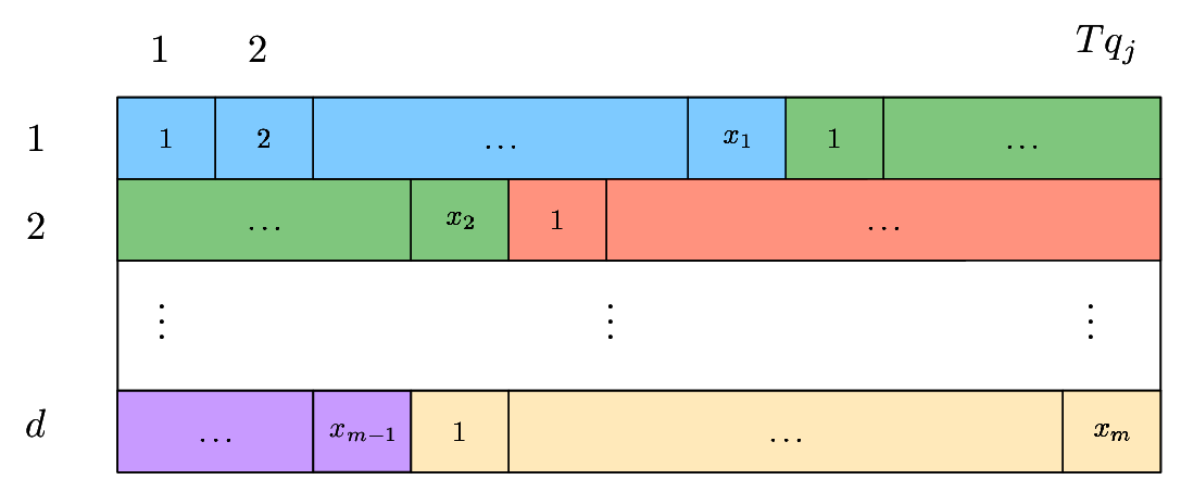
We next show how we can implement the optimal solution of problem (50). Suppose denote the optimal solution. Without loss of generality assume . The implementation is as follows. We allocate ad to the first ad slot of the first queries. We then allocate ad to the remaining first ad slots until we reach the last query (i.e., the -th query). We then allocate the remaining ads of type to the second ad slots of the initial queries. We continue this procedure until all ads are allocated. First note that all ads will be allocated because of the constraint . Moreover, the ads shown for each query are distinct. This is because of the way we fill out the slots and the fact that for all . Figure 4 illustrates this procedure.
References
- Adamczyk et al. [2016] Marek Adamczyk, Maxim Sviridenko, and Justin Ward. Submodular stochastic probing on matroids. Mathematics of Operations Research, 41(3):1022–1038, 2016.
- Andelman and Mansour [2004] Nir Andelman and Yishay Mansour. Auctions with budget constraints. In Scandinavian Workshop on Algorithm Theory, pages 26–38. Springer, 2004.
- Asadpour and Nazerzadeh [2015] Arash Asadpour and Hamid Nazerzadeh. Maximizing stochastic monotone submodular functions. Management Science, 62(8):2374–2391, 2015.
- Dobzinski and Schapira [2006] Shahar Dobzinski and Michael Schapira. An improved approximation algorithm for combinatorial auctions with submodular bidders. In Proceedings of the seventeenth annual ACM-SIAM symposium on Discrete algorithm, pages 1064–1073, 2006.
- Feige [2009] Uriel Feige. On maximizing welfare when utility functions are subadditive. SIAM Journal on Computing, 39(1):122–142, 2009.
- Feige et al. [2011] Uriel Feige, Vahab S Mirrokni, and Jan Vondrak. Maximizing non-monotone submodular functions. SIAM Journal on Computing, 40(4):1133–1153, 2011.
- Fleischer et al. [2006] Lisa Fleischer, Michel X Goemans, Vahab S Mirrokni, and Maxim Sviridenko. Tight approximation algorithms for maximum general assignment problems. In Proceedings of the seventeenth annual ACM-SIAM symposium on Discrete algorithm, pages 611–620, 2006.
- Gabillon et al. [2013] Victor Gabillon, Branislav Kveton, Zheng Wen, Brian Eriksson, and S Muthukrishnan. Adaptive submodular maximization in bandit setting. In Advances in Neural Information Processing Systems, pages 2697–2705, 2013.
- Goel and Mehta [2008] Gagan Goel and Aranyak Mehta. Online budgeted matching in random input models with applications to adwords. In Proceedings of the nineteenth annual ACM-SIAM symposium on Discrete algorithms, pages 982–991, 2008.
- Golovin and Krause [2011] Daniel Golovin and Andreas Krause. Adaptive submodularity: Theory and applications in active learning and stochastic optimization. Journal of Artificial Intelligence Research, 42:427–486, 2011.
- Goundan and Schulz [2007] Pranava R Goundan and Andreas S Schulz. Revisiting the greedy approach to submodular set function maximization. Optimization online, pages 1–25, 2007.
- Jones et al. [2006] Rosie Jones, Benjamin Rey, Omid Madani, and Wiley Greiner. Generating query substitutions. In Proceedings of the 15th international conference on World Wide Web, pages 387–396. ACM, 2006.
- Karp et al. [1990] Richard M Karp, Umesh V Vazirani, and Vijay V Vazirani. An optimal algorithm for on-line bipartite matching. In Proceedings of the twenty-second annual ACM symposium on Theory of computing, pages 352–358. ACM, 1990.
- Kempe et al. [2003] David Kempe, Jon Kleinberg, and Éva Tardos. Maximizing the spread of influence through a social network. In Proceedings of the ninth ACM SIGKDD international conference on Knowledge discovery and data mining, pages 137–146. ACM, 2003.
- Khot et al. [2005] Subhash Khot, Richard J Lipton, Evangelos Markakis, and Aranyak Mehta. Inapproximability results for combinatorial auctions with submodular utility functions. In International Workshop on Internet and Network Economics, pages 92–101. Springer, 2005.
- Lahaie et al. [2007] S Lahaie, D Pennock, A Saberi, and R Vohra. Algorithmic game theory, chapter sponsored search, 2007.
- Lehmann et al. [2006] Benny Lehmann, Daniel Lehmann, and Noam Nisan. Combinatorial auctions with decreasing marginal utilities. Games and Economic Behavior, 55(2):270–296, 2006.
- Li and Milenkovic [2017] Pan Li and Olgica Milenkovic. Inhomogeneous hypergraph clustering with applications. In Advances in Neural Information Processing Systems, pages 2305–2315, 2017.
- Lin and Bilmes [2011] Hui Lin and Jeff Bilmes. A class of submodular functions for document summarization. In Proceedings of the 49th Annual Meeting of the Association for Computational Linguistics: Human Language Technologies-Volume 1, pages 510–520, 2011.
- Malekian et al. [2008] Azarakhsh Malekian, Chi-Chao Chang, Ravi Kumar, and Grant Wang. Optimizing query rewrites for keyword-based advertising. In Proceedings of the 9th ACM conference on Electronic commerce, pages 10–19. ACM, 2008.
- Mehta [2013] Aranyak Mehta. Online matching and ad allocation. Foundations and Trends® in Theoretical Computer Science, 8(4):265–368, 2013.
- Mehta et al. [2007] Aranyak Mehta, Amin Saberi, Umesh Vazirani, and Vijay Vazirani. Adwords and generalized online matching. Journal of the ACM (JACM), 54(5):22, 2007.
- Mirzasoleiman et al. [2016] Baharan Mirzasoleiman, Amin Karbasi, Rik Sarkar, and Andreas Krause. Distributed submodular maximization. Journal of Machine Learning Research, 17(238):1–44, 2016.
- Mitrovic et al. [2018] Marko Mitrovic, Moran Feldman, Andreas Krause, and Amin Karbasi. Submodularity on hypergraphs: From sets to sequences. arXiv preprint arXiv:1802.09110, 2018.
- Mossel and Roch [2010] Elchanan Mossel and Sebastien Roch. Submodularity of influence in social networks: From local to global. SIAM Journal on Computing, 39(6):2176–2188, 2010.
- Nemhauser and Wolsey [1978] George L Nemhauser and Laurence A Wolsey. Best algorithms for approximating the maximum of a submodular set function. Mathematics of operations research, 3(3):177–188, 1978.
- Nemhauser et al. [1978] George L Nemhauser, Laurence A Wolsey, and Marshall L Fisher. An analysis of approximations for maximizing submodular set functions. Mathematical Programming, 14(1):265–294, 1978.
- Singh et al. [2012] Gyanit Singh, Nish Parikh, and Neel Sundaresan. Rewriting null e-commerce queries to recommend products. In Proceedings of the 21st International Conference on World Wide Web, pages 73–82. ACM, 2012.
- Singla et al. [2014] Adish Singla, Ilija Bogunovic, Gábor Bartók, Amin Karbasi, and Andreas Krause. Near-optimally teaching the crowd to classify. In ICML, pages 154–162, 2014.
- Tschiatschek et al. [2017] Sebastian Tschiatschek, Adish Singla, and Andreas Krause. Selecting sequences of items via submodular maximization. In AAAI, pages 2667–2673, 2017.
- Vondrák [2008] Jan Vondrák. Optimal approximation for the submodular welfare problem in the value oracle model. In Proceedings of the fortieth annual ACM symposium on Theory of computing, pages 67–74. ACM, 2008.
- Wolsey [1982] Laurence A Wolsey. Maximising real-valued submodular functions: Primal and dual heuristics for location problems. Mathematics of Operations Research, 7(3):410–425, 1982.
- Zhang and Jones [2007] Wei Vivian Zhang and Rosie Jones. Comparing click logs and editorial labels for training query rewriting. In WWW 2007 Workshop on Query Log Analysis: Social And Technological Challenges, 2007.