Exploiting Channel Memory for Joint Estimation and Scheduling in Downlink Networks
Abstract
We address the problem of opportunistic multiuser scheduling in downlink networks with Markov-modeled outage channels. We consider the scenario in which the scheduler does not have full knowledge of the channel state information, but instead estimates the channel state information by exploiting the memory inherent in the Markov channels along with ARQ-styled feedback from the scheduled users. Opportunistic scheduling is optimized in two stages: (1) Channel estimation and rate adaptation to maximize the expected immediate rate of the scheduled user; (2) User scheduling, based on the optimized immediate rate, to maximize the overall long term sum-throughput of the downlink. The scheduling problem is a partially observable Markov decision process with the classic ‘exploitation vs exploration’ trade-off that is difficult to quantify. We therefore study the problem in the framework of Restless Multi-armed Bandit Processes (RMBP) and perform a Whittle’s indexability analysis. Whittle’s indexability is traditionally known to be hard to establish and the index policy derived based on Whittle’s indexability is known to have optimality properties in various settings. We show that the problem of downlink scheduling under imperfect channel state information is Whittle indexable and derive the Whittle’s index policy in closed form. Via extensive numerical experiments, we show that the index policy has near-optimal performance.
Our work reveals that, under incomplete channel state information, exploiting channel memory for opportunistic scheduling can result in significant performance gains and that almost all of these gains can be realized using an easy-to-implement index policy.
I Introduction
The wireless channel is inherently time-varying and stochastic. It can be exploited for dynamically allocating resources to the network users, leading to the classic opportunistic scheduling principle (e.g., [1]). Understandably, the success of opportunistic scheduling depends heavily on reliable knowledge of the instantaneous channel state information (CSI) at the scheduler. Many sophisticated scheduling strategies have been developed with provably optimal characteristics (e.g., [2]-[6]) by assuming perfect CSI to be readily available, free of cost at the scheduler.
In realistic scenarios, however, perfect CSI is rarely, if ever, available and never cost-free, i.e., a non-trivial amount of network resource, that could otherwise be used for data transmission, must be spent in estimating the CSI [2]. This calls for jointly designing channel estimation and opportunistic scheduling strategies – an area that has recently received attention when the channel state is modeled by i.i.d. processes across time (e.g., [7], [8]). The i.i.d. model has traditionally been a popular choice for researchers to abstract the fading channels, because of its simplicity and associated ease of analysis. On the other hand, this model fails to capture an important characteristics of the fading channels – the time-correlation or the channel memory [2].
In the presence of estimation cost, memory in the fading channels is an important resource that can be intelligently exploited for more efficient, joint estimation and scheduling strategies. In this context, Markov channel models have been gaining popularity as realistic abstractions of fading channels with memory (e.g., [9]-[11]).
In this paper, we study joint channel estimation and scheduling using channel memory, in downlink networks. We model the downlink fading channels as two-state Markov Chains with non-zero achievable rate in both states. The scheduling decision at any time instant is associated with two potentially contradicting objectives: (1) Immediate gains in throughput via data transmission to the scheduled user; (2) Exploration of the channel of a downlink user for more informed decisions and associated throughput gains in the future. This is the classic ‘exploitation vs exploration’ trade-off often seen in sequential decision making problems (e.g., [12], [13]). We model the joint estimation and scheduling problem as a Partially Observable Markov Decision Process (POMDP) and study the structure of the problem, by explicitly accounting for the estimation cost. Specifically, our contributions are as follows.
We recast the POMDP scheduling problem as a Restless Multi-armed Bandit Process (RMBP) [14] and establish its Whittle’s indexability [14] in Section IV and V. Even though Whittle’s indexability is difficult to establish in general [15], we have been able to show it in the context of our problem.
Based on a Whittle’s indexability condition, we explicitly characterize the Whittle’s index policy for the scheduling problem in Section VI. Whittle’s index policies are known to have optimality properties in various RMBP processes and have been shown to be easy to implement (e.g., [15], [16]).
Using extensive numerical experiments, we demonstrate in Section VIII that Whittle’s index policy in our setting has near-optimal performance and that significant system-level gains can be realized by exploiting the channel memory for estimation and scheduling. Also, the Whittle’s index policy we derive is of polynomial complexity in the number of downlink users (contrast this with the PSPACE-hard complexity of optimal POMDP solutions [17]).
Our setup significantly differs from related works (e.g., [10] [11] [18]) in the following sense: In these works, the channels are modeled by ON-OFF Markov Chains with the OFF state corresponding to zero-achievable rate of transmission. There, once a user is scheduled, there is no need to estimate the channel of that user, since it is optimal to transmit at the constant rate allowed by the ON state irrespective of the underlying state. In contrast, in our model, the achievable rate at the lower state is, in general, non-zero and any rate above this achievable rate leads to outage. This extended model captures the realistic scenario when non-zero rates are possible with the use of sophisticated physical layer algorithms, even when the channel is bad. In this model, once a user is scheduled, the scheduler must estimate the channel of that user, with an associated cost, and adapt the transmission rate based on the estimate. The rate adaptation must balance between aggressive transmissions that lead to outage and conservative transmissions that lead to under-utilization of channels. The achievable rate expected from this process, in turn, influences the choice of the scheduled user. Thus the channel estimation and scheduling stages are tightly coupled, introducing several technical challenges to the problem, which we address in this paper.

II System Model and Problem Statement
II-A Channel Model
We consider a downlink system with one base station (BS) and users. Time is slotted with the time slots of all users synchronized. The channel between the BS and each user is modeled as a two-state Markov chain, i.e., the state of the channels remains static within each time slot and evolves across time slots according to Markov chain statistics. The Markov channels are assumed to be independent and, in general, non-identical across users. The state space of channel between the BS and user is given by . Each state corresponds to a maximum allowable data rate. Specifically, if the channel is in state , there exists a rate , , such that data transmissions at rates below succeed and transmissions at rates above fail, i.e., outage occurs. Similarly, state corresponds to data rate . Note that fixing the higher rate to be across all users does not impose any loss of generality in our analysis. This will be evident as we proceed.
The Markovian channel model is illustrated in Fig. 1. For user , the two-state Markov channel is characterized by a probability transition matrix
where

II-B Scheduling Model
We adopt the one-hop interference model, i.e., in each time slot, only one user can be scheduled for data transmission. At the beginning of the slot, the scheduler does not have exact knowledge of the channel state of the downlink users. Instead, it maintains a belief value for channel which is the probability that is in state at the time. We will elaborate on the belief values soon. Using these belief values, the scheduler picks a user, estimates its current channel state and subsequently transmits data at a rate adapted to the channel state estimate – all with an objective to maximize the overall sum-throughput of the downlink system. Specifically, in each slot, the scheduler jointly makes the following decisions: (1) Considering each user, the scheduler decides on the optimal channel estimator (that could involve the expenditure of network resources such as time, power, etc.) and rate adapter pair; (2) Based on the average rate of successful transmission promised for each user by the previous decision, the scheduler picks a user for channel estimation and subsequent data transmission. At the end of the slot, consistent with recent models (e.g., [10] [11] [18]), the scheduled user sends back accurate information on the state of the Markov channel in that slot. This accurate feedback is, in turn, used by the scheduler to update its belief on the channels, based on the Markov channel statistics. Note that these belief values are sufficient statistics to the past scheduling decisions and feedback [19]. Using to denote an arbitrary estimator and to denote an arbitrary rate adapter, as functions of the belief value , the basic operation is summarized in Fig. 2. The scheduling problem can be formulated as a partially observable Markov decision process [19], with the Markov channel states being the partially observable system states.
As noted in Section I, the scheduling decision in each slot involves two objectives: data transmission to the scheduled user and probing the channel of the scheduled user (through the accurate end-of-slot feedback). On one hand, the scheduler can transmit data to the user that promises the best achievable rate at the moment and hence realize immediate performance gains. On the other hand, the scheduler can schedule possibly another user and use the channel feedback from that user to gain a better understanding of the overall downlink system, which, in turn, could result in more informed future scheduling decisions with corresponding performance gains.
II-C Formal Problem Statement
We now proceed to formally introduce the expected immediate reward. We let denote the current belief value of the channel of user , and let denote an arbitrary estimator and rate adapter pair. Recall from the discussion on the scheduling model that, at the end of the slot, the scheduled user sends back accurate feedback on its Markov channel state in that slot. With this setup, once a user is scheduled, the choice of the channel estimator and rate adapter pair does not affect the future paths of the scheduling process. Thus, within each slot, it is optimal to design this pair to maximize the expected rate (of successful transmission) of the user scheduled in that slot. Henceforth, in the language of POMDPs, we call this maximized rate the expected immediate reward. We now proceed to formally introduce the expected immediate reward. We let denote the current belief value of the channel of user . The optimal estimator and rate adapter pair, , for user , when the belief is , is given by
| (1) |
where the quantity is the average rate of successful transmissions to user when the channel is in state and the estimator and rate adapter pair is deployed. The expectation in (1) is taken over the underlying channel state , with distribution characterized by belief value , i.e.,
The expected immediate reward when user is scheduled is thus given by
| (2) |
Note that our model is very general in the sense that we do not restrict to any specific estimation, data transmission structure or to any specific class of estimators. A typical estimation, data transmission structure, corresponding to the estimator and rate adapter pair is illustrated in Fig. 3. Here a pilot-aided training[2]-based estimation is performed for a fraction of the time slots followed by data transmission at an adapted rate in the rest of the time slots.

We now introduce the optimality equations for the scheduling problem. Let denote the vector of current belief values of the channels at the beginning of slot . A stationary scheduling policy, , is a stationary mapping between the belief vector and the index of the user scheduled for data transmission in the current slot. Our performance metric is the infinite horizon, discounted sum-throughput of the downlink (henceforth simply the expected discounted reward in the language of POMDPs), formally defined next.
For a stationary policy , the expected discounted reward under initial belief is given by
where is the belief vector in slot , denotes the belief value of user in slot , , denotes the index of the user scheduled in slot . The discount factor provides relative weighing between the immediately realizable rates and future rates. For any initial belief , the optimal expected discounted reward, , is given by the Bellman equation [20]
Here denotes the belief vector in the next slot when the current belief is . The belief evolution proceeds as follows:
| (3) |
where is the belief evolution operator for user when it is not scheduled in the current slot. A stationary scheduling policy is optimal if and only if for all [20].
In the introduction, we briefly contrasted our setup with those in [10][11][18]. We provide a rigorous comparison here. The works [10][11][18] studied opportunistic scheduling with the channels modeled by ON-OFF Markov chains. In these works, the lower state is an ‘OFF’ state, i.e., it does not allow transmission at any non-zero data rate. Contrast this with our model where, at the lower state , a possibly non-zero rate is achievable and outage occurs at any rate above . We now further explain how these two models are fundamentally different.
In the ON-OFF channel model, the scheduler does not need a channel estimator and rate adapter pair. The scheduler can aggressively transmit at rate , since it has nothing to gain by transmitting at a lower rate – a direct consequence of the ‘OFF’ nature of the lower state. On the other hand, transmitting at a rate lesser than can lead to losses due to under-utilization of the channel.
In contrast, in our model, when , the scheduler must strike a balance between aggressive and conservative rates of transmission. An aggressive strategy (transmit at rate ) can lead to losses due to outages, while a conservative strategy can lead to losses due to under-utilization of the channel. This underscores the importance of the knowledge of the underlying channel state and, therefore, the need for intelligent estimation and rate adaptation mechanisms.
As a direct consequence of the preceding arguments, the expected immediate reward in our model is not a trivial -shift of the expected immediate reward when the rates supported by the channel states are and . Formally,
where is the immediate reward when the channel state space is and belief value of the scheduled user is . In fact, it can be shown that (in Lemma 1)
We believe that, our channel model, in contrast to the ON-OFF model, better captures realistic communication channels where, using appropriate physical layer algorithms, it is possible to transmit at a non-zero rate even at the lowest state of the channel model and the same physical layer algorithms may impose outage behavior when this allowed rate is exceeded.
III Optimal Expected Transmission Rate – Structural Properties
In this section, we study the structural properties of the expected immediate reward, , defined in Equation (2). These properties will be crucial for our analysis in subsequent sections. For notational convenience, we will drop the suffix in the rest of this section.
Lemma 1.
The expected immediate reward has the following properties:
(a) is convex and increasing in for
(b) is bounded as follows:
| (4) |
Proof: Let be the set of optimal estimator and rate adapter pairs for all , i.e., . The expected immediate reward, provided in (2), can now be rewritten as
where denotes the average rate of successful transmission when the channel state is . Note that, for fixed , the average rate is linear in . Thus, is given as a point-wise maximum over a family of linear functions, which is convex [21]. is therefore convex in , establishing the convexity statement in (a).
We next proceed to derive the bounds to . From Equation (2),
where indicates that we are considering rate adaptation without channel estimation. This explains the last inequality. Note that without the estimator, the rate adaptation is solely a function of the belief value . Thus, the average rate achieved under the rate adapter, conditioned on the underlying channel state, can be expressed simply by indicator functions, as seen below:
This establishes the lower bound in (b).
The upper bound in (b) corresponds to the expected immediate reward when full channel state information is available at the scheduler.
It is clear from the upper and lower bounds that . Note that when or , there is no uncertainty in the channel, hence and . Using these properties, along with the convexity property of , we see that is monotonically increasing in , establishing the monotonicity of (a). The lemma thus follows.
Remark: Here we present some insights into the effect of the non-zero rate on the channel estimation and rate adaptation mechanisms by studying the upper and lower bounds to provided in Lemma 1. The upper bound essentially corresponds to the case when perfect channel state information is available at the scheduler at the beginning of each slot. Here, no channel estimation and rate adaptation is necessary. The lower bound, on the other hand, corresponds to the case when the channel estimation stage is eliminated and rate adaptation is performed solely based on the belief value of the scheduled user.
Fig. 4 plots the lower and upper bounds to for different values of . Note that the lower bound approaches the upper bound in both directions, i.e., when or when . This behavior can be explained as follows: (1) essentially means that the states of the Markov channel move closer to each other. This progressively reduces the channel uncertainty and hence the need for channel estimation (and, consequently, rate adaptation), essentially bringing the bounds closer. (2) As , the channel uncertainty increases. At the same time, the impact of the channel estimator and rate adapter pair decreases. This is because, as , the loss in immediate reward due to outage (transmitting at when channel is in state ) is less severe than the loss due to under-utilization of the channel (transmitting at rate when the channel is in state ), essentially making it optimal for the rate adaptation scheme to be progressively more aggressive (transmit at rate ). Thus channel estimation loses its significance as . This brings the bounds closer as .
It can be verified that the separation between the lower and upper bounds is at its peak when . This, along with the preceding discussion, indicates the potential for rate improvement when intelligent channel estimation and rate adaptation is performed under moderate values of .

IV Restless Multi-Armed Bandit Processes, Whittle’s Indexability and Index Policies
A direct analysis of the downlink scheduling problem appears difficult due to the complex nature of the ‘exploitation vs exploration’ tradeoff. We therefore establish a connection between the scheduling problem and the Restless Multiarmed Bandit Processes (RMBP) [14] and make use of the established theory behind RMBP in our analysis. We briefly overview RMBPs and the associated theory of Whittle’s indexability in this section.
RMBPs are defined as a family of sequential dynamic resource allocation problems in the presence of several competing, independently evolving projects. In RMBPs, a subset of the competing projects are served in each slot. The states of all the projects in the system stochastically evolve in time based on the current state of the projects and the action taken. Once a project is served, a reward dependent on the states of the served projects and the action taken is accrued by the controller. Hence, the RMBPs are characterized by a fundamental tradeoff between decisions guaranteeing high immediate rewards versus those that sacrifice immediate rewards for better future rewards. Solutions to RMBPs are, in general, known to be PSPACE-hard [17].
Under an average constraint on the number of projects scheduled per slot, a low complexity index policy developed by Whittle [14], commonly known as Whittle’s index policy, is optimal. Under stringent constraint on the number of users scheduled per slot, Whittle’s index policy may not exist and if it does exist, its optimality properties are, in general, lost. However, Whittle’s index policies, upon existence, are known to have near optimal performance in various RMBPs (e.g., [15] [16]). For an RMBP, Whittle’s index policy exists if and only if the RMBP satisfies a condition known as Whittle’s indexability [14], defined next.
Consider the following setup: for each project in the system, consider a virtual system where, in each slot, the controller must make one of two decisions: (1) Serve project and accrue an immediate reward that is a function of the state of the project. This reward structure reflects the one in the original RMBP for project . (2) Do not serve project , i.e., stay passive and accrue an immediate reward for passivity . The state of the project evolves in the same fashion as it would in the original RMBP, as a function of its current state and current action (whether is served or not in the current state). Let be the set of states of project in which it is optimal to stay passive, where optimality is defined based on the infinite horizon net reward.
Project is Whittle indexable if and only if as increases from to , the set monotonically expands from to , the state space of project . The RMBP is Whittle indexable if and only if all the projects in the RMBP are Whittle indexable.
For each state, , of a project, Whittle’s index, , is given by the value of in which the net reward after both the active and passive decisions are the same in the -subsidized virtual system. The notion of indexability gives a consistent ordering of states with respect to the indices. For instance, if and if it is optimal to serve the project at state , then it is optimal to serve the project at . This natural ordering of states based on indices renders the near-optimality properties to Whittle’s index policy (e.g., [15], [16]).
The downlink scheduling problem we have considered is in fact an RMBP process. Here, each downlink user, along with the belief value of its channel, corresponds to a project in the RMBP, and the project is served when the corresponding user is scheduled for data transmission. Now, referring to our earlier discussion on the RMBPs, we see that Whittle’s index policy is very attractive from an optimality point of view. The attractiveness of the index policy can be attributed to the natural ordering of states (and hence projects) based on indices, as guaranteed by Whittle’s indexability. In the rest of the paper, we establish that this advantage carries over to the downlink scheduling problem at hand. As a first step in this direction, in the next section, we study the scheduling problem in Whittle’s indexability framework and show that the downlink scheduling problem is, in fact, Whittle indexable.
V Whittle’s Indexability Analysis of the Downlink Scheduling Problem
In this section, we study the Whittle’s indexability of our joint scheduling and estimation problem. To that end, we first describe the downlink scheduling setup:
At the beginning of each slot, based on the current belief value (we drop the user index in this section since only one user is considered throughout), the scheduler takes one of two possible actions: schedules data transmission to the user (action ) or stays idle (). Upon an idle decision, a subsidy of is obtained. Otherwise, optimal channel estimation and rate adaptation is carried out, with a reward equal to (consistent with the immediate reward seen in previous sections). The belief value is updated based on the action taken and feedback from the user (upon transmit decision). This belief update is consistent with that in the Section II. The optimal scheduling policy (henceforth, the -subsidy policy) maximizes the infinite horizon discounted reward, parameterized by . The optimal infinite horizon discounted reward is given by the Bellman equation [20]
| (5) |
where, recall from Section II, is the evolution of the belief value when the user is not scheduled. The first quantity inside the operator corresponds to the infinite horizon reward when a transmit decision is made in the current slot and optimal decisions are made in the future slot. The second element corresponds to idle decision in the current slot and optimal decisions in all future slots.
We note that the indexability analysis in the rest of this section bears similarities to that in [18], where the authors studied indexability of a sequential resource allocation problem in a cognitive radio setting. This problem is mathematically equivalent to our downlink scheduling problem when . We have already discussed in detail (in Section II) that the structure of the immediate reward when is very different than when , due to the need for channel estimation and rate adaptation in the former case. Consequently, in the Whittle’s indexability setup, the infinite horizon discounted reward in our problem is different (and more general) than that in [18], underscoring the significance of our results.
As a crucial preparatory result, we now proceed to show that the -subsidy policy is thresholdable.
V-A Thresholdability of the -subsidy policy
We first record our result on the convexity property of the infinite horizon discounted reward, , of (5) in the following proposition.
Proposition 1.
The infinite horizon discounted reward, is convex in .
Proof: We first consider the discounted reward for finite horizon -subsidy problem. We let and represent the immediate reward corresponding to active and idle decisions, respectively. The reward function associated with -stage finite horizon process is expressed as
Let be the reward at time with belief value . Hence and the last stage value function is given by
Therefore, is convex with since it is the maximum of a constant and a convex function. For any time , the Bellman ([20]) equation can be written as
where
| (6) | ||||
| (7) |
Suppose now is convex with . If , it is clear from (7) that is convex function of since it is a summation of a convex function and a linear function of . If , , expressed in (6), is also a convex function, because composition of convex function and linear function is convex [21]. Therefore is convex with as maximum of two convex functions. By induction, the convexity of is thus established.
Since , is convex with . For discounted problem with bounded reward per slot, the infinite horizon reward is the limit of of finite horizon reward ([20]). Therefore . Upon point-wise convergence, point-wise limit of convex functions is convex [21]. Hence is a convex function of .
| (11) |
In the next proposition, we show that the optimal -subsidy policy is a threshold policy.
Proposition 2.
The optimal -subsidy policy is thresholdable in the belief space . Specifically, there exists a threshold such that the optimal action is if the current belief and the optimal action is , otherwise. The value of the threshold depends on the subsidy , partially characterized below.
(i) If , ;
(ii) If , for some arbitrary ;
(iii) If , takes value within interval .
Proof: Consider the Bellman equation (5), let be the reward corresponding to transmit decision and be the reward corresponding to idle decision, i.e.,
| (8) | ||||
| (9) |
It is clear from the Bellman equation (5) that the optimal action depends on the relationship between and , presented as follows.
Case (i). If , since , in each slot, the immediate reward for being idle always dominates the reward for being active. Hence it will be optimal to always stay idle. We can thus set the threshold to 1.
Case (ii). If , then for any , we have
where the inequality is due to along with Jensen’s inequality [21] due to the convexity of from Proposition 2. Hence, it is optimal to stay active. Consistent with the threshold definition, we can set for any .
Case (iii). If , then at the extreme values of belief,
Note that the relationship of and is reversed at the end points and , and they are both convex functions of . Thus, there must exist a threshold within such that equals 1 whenever .
V-B Whittle’s Indexability of Downlink Scheduling
Having established that the -subsidy policy is thresholdable in Proposition 2, Whittle’s indexability, defined in Section IV, is re-interpreted for the downlink scheduling problem as follows: the downlink scheduling problem is Whittle indexable if the threshold boundary is monotonically increasing with subsidy .
Using our discussion in Section IV, the index of the belief value , i.e., is the infimum value of the subsidy such that it is optimal to stay idle, i.e.,
| (10) |
To establish indexability, we need to investigate the infinite horizon discounted reward , given by (5). We can observe from (5) that given the value of and , can be calculated for all . Let denote the steady state probability of being in state . The next lemma provides a closed form expression for and and is critical to the proof of indexability.
Lemma 2.
The discounted rewards and can be expressed as:
Case 1: (positive correlation)
Case 2: (negative correlation)
Proof: The derivation of and follows from substituting and in Equation (5). Together with the expression of given by in Section II, the expression of and can be obtained. For details, please refer to Appendix A.
We note that the value function expression depends on the correlation type of the Markov chain, because the transition function given in Section II will behave differently with the correlation type of the chain.
The closed form expression of the value function given by the previous lemma serves as a useful tool for us to establish indexability, which is given by the next proposition.
Proposition 3.
The threshold value is strictly increasing with . Therefore, the problem is Whittle indexable.
VI Whittle’s Index Policy
VII Whittle’s Index Policy and Numerical Performance Analysis
In this section, we explicitly characterize Whittle’s index policy for the downlink scheduling problem. For user , let denote the steady state probability of being in state , and let denote the reward function for its -subsidy problem in (5). We first characterize the Whittle’s index as follows.
Proposition 4.
For user , the index value at state , i.e., is characterized as follows,
Case 1. Positively correlated channel ()
Case 2. Negatively correlated channel ()
Proof: The derivation of the index value follows from substituting the expression of and (given in Lemma 2) into Equation (5). Details of the proof are provided in Appendix C.
Remark: Notice that Proposition 4 does not give the closed form expression for . However, since the closed form expression of the value function and are derived in Lemma 2, closed form expressions of can be easily calculated and is given in Appendix C. We now introduce Whittle’s index policy.
Whittle’s Index Policy: In each slot, with belief values , the user with the highest index value is scheduled for transmission, i.e., .


Note that, from the definition of indexability, the index value monotonically increases with . Therefore, when the Markovian channels have the same Markovian structure and vary independently across users (hence the state-index mappings are the same across users), Whittle’s index policy essentially becomes the greedy policy – schedule the user with the highest belief value.
Fig. 5 plots an example of the index value evolution for the case of positively correlated and negatively correlated channels when they stay idle, i.e., not scheduled for transmission. We see that, for the positively correlated channel, the index value behaves monotonically, while, for the negatively correlated channel, the index value shows oscillation. This resembles the evolution of the belief values, which, as proven in Lemma 3 in Appendix A, approaches steady state monotonically for the positively correlated channel, and with oscillation for the negatively correlated channel. This resemblance in Fig. 5 is expected since, from Proposition 3, we can infer that the index value monotonically increases with the belief value. Thus, in essence, from Proposition 3 and Fig. 5, we see that the index value captures the underlying dynamics of the Markovian channel.

VIII Numerical Performance Analysis
VIII-A Model for Simulation
In this section, we study, via numerical evaluations, the performance of Whittle’s index policy, henceforth simply the index policy, for joint estimation and scheduling in our downlink system. We consider the specific class of estimator and rate adapter structure, with pilot-aided training, discussed in Section II and illustrated in Fig. 3. We consider a fading channel with the fading coefficients quantized into two levels to reflect the two states of the Markov chain. Additive noise is assumed to be white Gaussian. The channel input-output model is given by , where correspond to transmitted and received signals, respectively, is the complex fading coefficient and is the complex Gaussian, unit variance additive noise. Conditioned on , the Shannon capacity of the channel is given by . We quantize the fading coefficients such that the allowed rate at the lower state, for all users. The channel state, represented by the fading coefficient, evolves as Markov chain with fading block length .
We consider a class of Linear Minimum Mean Square Error (LMMSE) estimators [22] denoted as . LMMSE estimators are attractive because with additive white Gaussian noise, they can be characterized in closed form [22] and, hence, can be conveniently used in simulation. Let denote the optimal LMMSE estimator with prior . We let denote the set of LMMSE estimators optimized for various values of .
VIII-B Immediate Reward Structure
We now study the structure of the immediate reward . Note that is optimized over the class of estimators . Fig. 6 illustrates , in comparison with the upper and lower bounds derived in Lemma 2, for two values of block length . As established in Lemma 2, shows a convex increasing structure and takes values within the bounds. Note that also increases with , since a larger provides more channel uses for channel probing and data transmission.
VIII-C Near-optimal Performance of Whittle’s Index Policy
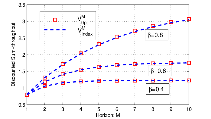
We proceed to evaluate the performance of the index policy and compare it with the optimal policy. In Fig. 7, we compare the expected rewards and that, respectively, correspond to the optimal finite M-horizon policy and the index policy, for increasing horizon length and randomly generated system parameters. The value of is obtained via brute-force search over the finite horizon. Fig. 7 illustrates the near optimal performance of the index policy. Also, as expected, the higher the value of , the higher the expected reward.
Table I presents the performance of the index policy in a larger perspective. Here, with randomly generated system parameters, the infinite horizon reward under the index policy is compared with those of the optimal policy and a policy that ‘throws away’ the feedback from the scheduled user. Let denote the reward under this ‘no feedback’ policy. The infinite horizon rewards are obtained as limits of the finite horizon until convergence is achieved. The high values of the quantity gain, in addition to underscoring the near-optimality of the index policy, also signifies the high system-level gains from exploiting the channel memory using the end-of-slot feedback.
| gain | |||||
|---|---|---|---|---|---|
| 4 | 0.6337 | 1.6289 | 1.6289 | 1.4887 | 100 |
| 4 | 0.5896 | 1.5977 | 1.5866 | 1.2888 | 96.4045 |
| 4 | 0.6673 | 1.6537 | 1.6319 | 1.4342 | 90.0500 |
| 5 | 0.4537 | 0.9854 | 0.9854 | 0.9299 | 100 |
| 5 | 0.6082 | 1.6132 | 1.6072 | 1.4777 | 95.5518 |
| 5 | 0.6537 | 2.3728 | 2.3725 | 2.1494 | 99.8697 |
| 5 | 0.5397 | 1.6330 | 1.6330 | 1.5961 | 100 |
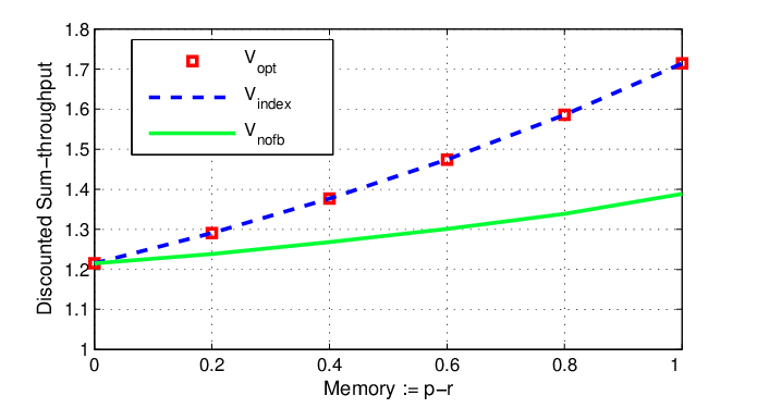
In Fig. 8 we study the effect of the channel ‘memory’ on the performances of various baseline policies. We consider five users with statistically identical but independently varying channels. Thus , , . We define the channel ‘memory’ as the difference and increase the memory by increasing from to and maintaining . Note that, with this approach, . Under this condition, the steady state probability that a channel is in the higher state is kept constant under varying channel memory. This, essentially, provides a degree of fairness between systems with different channel memories. Fig. 8 compares the rewards , and that respectively correspond to the rewards under the optimal policy, the index policy, and the ‘no feedback’ policy introduced earlier, for increasing channel memory. Note that when , the channel of each user evolves i.i.d. across time, with no information contained in the channel state feedback. Thus the policy that throws away this feedback achieves the same performance as the optimal policy that optimally uses this feedback, i.e., when . Also, since the channels are i.i.d. across users, when , the index policy simplifies to a ‘randomized’ policy that schedules randomly and uniformly across users, in effect mirroring the ‘no feedback’ policy in this setting. This explains when . As the channel memory increases, the significance of the channel state feedback increases, resulting in an increasing gap between the policies that use this feedback (optimal and Whittle’s index policies) and the ‘no feedback’ policy.
Fig. 8, along with Table I, shows that exploiting channel memory for opportunistic scheduling can result in significant performance gains, and almost all of these gains can be realized using the easy-to-implement index policy.
IX Conclusion
In this paper, we have studied downlink multiuser scheduling under a Markov-modeled channel. We considered the scenario in which the channel state information is not perfectly known at the scheduler, essentially requiring a joint design of user selection, channel estimation and rate adaptation. This calls for a two-stage optimization: (1) Within each slot, the channel estimation and rate adaptation is optimized to obtain an optimal transmission rate in the scheduling slot; (2) Across scheduling slots, users are selected to maximize the infinite horizon discounted reward. We formulated the scheduling problem as a partially observable Markov decision processes with the classic ‘exploitation versus exploration’ trade-off. We then linked the problem to a restless multiarmed bandit processes and conducted a Whittle’s indexability analysis. By obtaining structural properties of the optimal reward within the indexability setup, we showed that the downlink scheduling problem is Whittle indexable. We then explicitly characterized the Whittle’s index policy and studied the performance of this policy using extensive numerical experiments, which suggest that the index policy has near optimal performance and significant system level gains can be realized by exploiting the channel memory for joint channel estimation and scheduling.
Appendix A Proof of Lemma 2
We first establish structural properties of the belief update when a user stays idle. Suppose a user has the initial belief value and stays idle at all times, the belief value at slot is then given by , where is the iteration of function , given by
| (12) |
We let be the steady state distribution of the two-state channel being at the higher state, i.e.,
It is clear that An example of the belief evolution when a user stays idle is depicted in Fig. 9. This figure shows that, when staying idle, the belief value approaches steady state monotonically for positively correlated channel and approaches steady state with oscillation for negatively correlated channel. The structural properties of is critical to the rest of the proof and is recorded in the following lemma.
Lemma 3.
(i) For positively correlated channel (i.e., ), converges to steady state monotonically. For negatively correlated channel (i.e., ), converges to steady state with oscillation and a monotonically converging envelope.
(ii) for all and .
| (14) |
Proof: (i) Since we have for positively correlated channel and for negatively correlated channel, it is clear from the expression of (12) that converges to steady state monotonically and approaches steady state with oscillation and a monotonically converging envelop.
(ii) Since we have established part (i), it suffices to check that the first step transition satisfies: , for all , as shown below.
For positively correlated channel, since
For negatively correlated channel, since ,
The lemma is thus proved.


We then define as the time needed for belief value of a user to exceed from below, starting from initial value . Formally,
Positive correlation ()
Negative correlation ()
We shall refer to the ‘active set’ as the set of belief values for which the optimal decision is to transmit. The ‘idle set’ denotes the set of belief values for which the optimal decision is to stay idle. We proceed to derive the value functions and based on the value of .
(1) Positive correlation ().
When , the belief value is thus in the ‘idle set’. From Lemma 3(ii), if , the system stays idle. Hence the reward function is expressed as
When , the belief value is then in the ‘active set’. Hence from the Bellman equation in (5),
Rearranging the terms yields,
When , the value is then in ‘active set’. From Lemma 3(ii), regardless of the scheduling decision, the belief values , starting from , stays in the ‘active set’. Therefore
When , since , the belief value is in ‘idle set’. From Lemma 3(i), the belief values , starting from , stays in ‘idle set’. Hence
When , the belief value is therefore in ‘idle set’. Since the channel is positively correlated, from Lemma 3, starting from , the user remains idle for a duration of slots. Therefore
| (13) |
where
(2) Negative correlation ().
The derivation of and for negative correlation case follows an approach similar to that for the case of positive correlation. Details are, therefore, omitted here.
Note that the expressions of the value functions and in Lemma 2 are not in closed form. However, the closed form expressions for and can be easily calculated based on the expressions in Lemma 2, recorded below.
Case (1) Positive correlation (). First we give the closed form expression of .
If ,
If ,
If ,
We proceed to give the closed form expression of .
If ,
If , is given in equation (14).
If , .
Case (2) Negative correlation (). In this case, the closed form expression of is given as follows.
If , then
If , then
If , we have
If , then
Then we give the closed form expression of .
If , then
If , we have
If , then
Appendix B Proof of Proposition 3
We prove that the problem is Whittle indexable by showing that monotonically increases with . It is clear from Proposition 2 that for . So it suffices to show that is strictly increasing for . The proof technique follows along the lines of [18] and is presented next. We first proceed with the following lemma, where the right derivative of the reward function is compared.
Lemma 4.
If for all , we have
| (15) |
then is strictly increasing with for .
Proof: The lemma is proven by contradiction. Suppose there exists , such that is decreasing (i.e., non-increasing) at , hence it is decreasing in a neighborhood of , say, . Since and is decreasing at , is within the ‘active set’ for the -subsidy problem. Therefore we have . Besides, from the definition of threshold value , . Therefore,
which contradicts with the assumption.
Therefore, to establish indexability, it suffices to prove the inequality (15), i.e., . Let be the discounted time the -subsidy process, with initial belief , is made passive, i.e.,
Noting that giving the value of , the studying the belief value evolution follows the same pattern as in ON/OFF channel case, hence the expression of takes the same form as given in [18]. It follows from [14][18] that . Taking derivative of the and expressions (8)-(9) with respect to , the objective (15) now becomes
| (16) |
Case (1) If , from Lemma 3(ii), starting from the initial belief value or , the believe value never evolves below , hence the project is active at all times under optimal control. Therefore . Equation (16) thus holds.
| (21) |
| (22) |
| (26) |
| (27) |
Case (2) If , starting from initial belief , the belief value always stays within the ‘idle set’, i.e., . Equation (16) holds since and, similarly, .
We then discuss (17) separately for negatively and positively correlated channels.
Negatively correlated channel (). Since , the belief value is in the ‘active set’, hence
Therefore, we have
| (18) |
Following the same technique as in [18], the above inequality can be verified by substituting by and by .
Positively correlated channel (). In this case, is in the ‘active set’, hence
Taking derivative with respect to we have,
| (19) |
We note that the expression of takes the same form as in [18]. By applying the same technique as in [18], it can be checked that the above inequality indeed holds.
Therefore the inequality (16) is justified and hence indexability holds.
Appendix C Proof of Proposition 4
For -subsidy problem of user , from indexability, we know that strictly increases from to as increases from to . Hence the index value, from its definition in (10), is the subsidy value for which the active and idle decisions are equally attractive. We can hence derive index value by equating and and solve for as a function of , i.e.,
| (20) |
Note that the expressions of and have been given by Lemma 2. Substituting in (20) the values of and , we obtain the index value expressions, explained in the following.
Case (1). Positively correlation ().
If , the belief value , , are in the ‘idle set’ and, starting from initial belief or , or , will stay in the ‘idle set’. Hence
Substituting the above expressions in (20) we obtain that .
If , then is in ‘active set’, and starting from initial belief or , stays within ‘idle set’ at all times. Hence
If , then the value is in the ‘active set’. Therefore,
Again, substituting the expression of in (20), we have
Case (2). Negative correlation ().
Using the similar approach as in the positive correlation case, the expressions of the index value can be derived for the case of negative correlation, which are given in the Proposition 4. Details are, therefore, omitted here.
Note that the expressions given in Proposition 4 are not in closed form. However, the closed form expression for the index value can be easily calculated based on these expressions provided in Proposition 4, recorded as follows.
Case (1). Positively correlated channel ().
If , then the index value .
If , then
If , is given in (21), where
If , the index value is given in (22).
Case (2). Negatively correlated channel (.)
If , we have
If , then
If , the index value is expressed as
where
| (23) | ||||
| (24) | ||||
| (25) |
If , the index value is given in equation (27).
References
- [1] R. Knopp, P. A. Humblet, “Information capacity and power control in single cell multiuser communications,” in IEEE International Conference on Communications, 1995.
- [2] D. Tse, P. Viswanath, “Fundamentals of wireless communication,” Cambridge University Press, 2005.
- [3] L. Tassiulas, “Scheduling and performance limits of networks with constantly changing topology,” IEEE Transactions on Information Theory, 1997.
- [4] M. Neely, E. Modiano, C. Rohrs, “Dynamic power allocation and routing for time varying wireless networks,“ IEEE Journal on Selected Areas in Communications, vol. 23, pp. 89–103, 2005.
- [5] S. Shakkottai, A. Stolyar, “Scheduling for multiple flows sharing a time-varying channel: the exponential rule,” American Mathematical Society Translations, vol. 207, pp. 185–202., 2002.
- [6] A. Eryilmaz, R. Srikant, “Fair Resource Allocation in Wireless Networks using Queue-length based Scheduling and Congestion Control,” IEEE/ACM Transactions on Networking, vol. 15, pp. 1333–1344, 2007.
- [7] M. J. Neely, “Max weight learning algorithms with application to scheduling in unknown environments,” arXiv preprint:0902.0630, 2009.
- [8] C. Thejaswi, J. Zhang, S. Pun, V. H. Poor, “Distributed Opportunistic Scheduling with Two-Level Channel Probing,” IEEE/ACM Transactions on Networking, vol. 18, pp.1464–1477, 2009.
- [9] L. A. Johnston, V. Krishnamurthy, “Opportunistic file transfer over a fading channel: a POMDP search theory formulation with optimal threshold policies,” IEEE Transactions on Wireless Communications, vol.5, pp. 394–405, 2006.
- [10] S. Murugesan, P. Schniter, N. B. Shroff, “Multiuser Scheduling in a Markov-modeled Downlink using Randomly Delayed ARQ Feedback,” arXiv preprint:1002.3312, 2010.
- [11] S. H. Ahmad, M. Liu, T. Javidi, Q. Zhao, B. Krishnamachari, “Optimality of myopic sensing in multi-channel opportunistic access,” IEEE Transactions on Information Theory, vol. 55, pp. 4040–4050, 2009.
- [12] C. Safran, C. G. Chute, “Exploration and exploitation of clinical databases”, International Journal of Bio-Medical Computing, vol. 39, pp. 151–156, 1995.
- [13] L.P. Kaelbling, M.L. Littman, A.W. Moore, “Reinforcement learning: a survey,” Journal of Artificial Intelligence Research, vol. cs.AI/9605, pp. 237–285, 1996.
- [14] P. Whittle, “Restless Bandits: Activity Allocation in a Changing World,” Journal of Applied Probability, vol. 25, pp. 287–298. 1988.
- [15] K.D. Glazebrook, H.M. Mitchell, P.S. Ansell “Index policies for the maintenance of a collection of machines by a set of repairmen,” European Journal of Operational Research, vol. 165, pp. 267–284, 2005.
- [16] P. S. Ansell, K. D. Glazebrook, J. Nino-Mora, M. O’Keeffe “Whittle’s index policy for a multi-class queueing system with convex holding costs,” Mathematical Methods of Operations Research, vol. 57, pp. 21–39, 2003.
- [17] C. Papadimitriou, J.N. Tsitsiklis “ The complexity of optimal queueing network control ,” Mathematics of Operation Research, vol. 24, pp. 293–305, 1999.
- [18] K. Liu and Q. Zhao “Indexability of Restless Bandit Problems and Optimality of Whittle’s Index for Dynamic Multichannel Access,” IEEE Transactions on Information Theory, vol. 56, pp. 5547-5567, 2010.
- [19] E. J. Sondik, “The optimal control of partially observable Markov Decision Processes,” PhD thesis, Stanford University, 1971.
- [20] D. P. Bertsekas “Dynamic Programming and Optimal Control, vol. 1 and 2” Athena Scentific, Belmount, Massachusetts,2005.
- [21] S. Boyd, L. Vandenberghe, “Convex optimization,” Cambridge University Press, 2004.
- [22] T. Kailath, A. Sayed, B. Hassibi, “Linear estimation,”, Prentice Hall, 2000.