FZJ-IKP-TH-2010-21, HISKP-TH-10/25
The reaction in a unitary coupled-channels model
Abstract
Elastic scattering and the reaction are described simultaneously in a unitary coupled-channels approach which respects analyticity. SU(3) flavor symmetry is used to relate the - and - channel exchanges that drive the meson-baryon interaction in the different channels. Angular distributions, polarizations, and spin-rotation parameters are compared with available experimental data. The pole structure of the amplitudes is extracted from the analytic continuation.
Keywords:
Baryon spectroscopy , Resonance separation , Jülich modelPACS
11.30.Hv , 11.80.Gw , 13.75.Gx , 14.20.Gk , 24.10.Eq1 Introduction
The excitation spectrum of baryons and mesons is expected to reveal important information on the mechanism of confinement as well as the intrinsic structure of hadrons. Properties of baryon resonances have been obtained by lattice calculations [1, 2, 3, 4], mostly for the ground states but also for some excited states [2, 3]. In quark models [5, 6, 7], a rich spectrum of excited states is predicted. Many of these resonances could be identified in elastic scattering, while at higher energies, usually more states are predicted than seen, a fact commonly referred to as the “missing resonance problem” [8]. Since resonances not seen in the channel might predominantly couple to other channels, there are intensive experimental efforts [9] to measure, among others, multi-pion or final states, where or .
The reaction provides access to a pure isospin two-body reaction channel in meson-nucleon dynamics. Moreover, the weak decay allows to determine the polarization of the produced . In the 1980’s, Candlin et al. measured differential cross sections and polarizations at the Rutherford Appleton Laboratory for pion beam momenta ranging from GeV/c to GeV/c [10] and performed an energy-dependent isobar analysis for invariant collision energies ranging from the threshold ( GeV) to GeV [11]. While the quality of the fit is good, unitarity is violated and a separation of the resonant part is difficult due to the oversimplified construction of the partial wave amplitudes. The resonance parameters extracted confirmed four -resonances found previously in the partial wave analyses of elastic pion-nucleon scattering by Cutkosky et al. [12] and Höhler et al. [13, 14], the , , , and . Other resonances deduced from elastic pion-nucleon scattering by Refs. [12, 13, 14] could not be unambiguously identified in production [11], notably the , which is given a 4-star status by the PDG, and the , downsized to a one star rating (nowadays, two star) after the data became available.
In 1988, Candlin et al. [15] measured the spin-rotation parameter at the CERN-SPS, using a polarized frozen spin target and the Rutherford Multiparticle Spectrometer RMS, adding independent information to the data base for two pion beam momenta GeV/c and GeV/c. The spin-rotation parameter correlates the spin of the target proton and the spin of the produced and allows to eliminate ambiguities in the partial wave analysis. Discrepancies between the -values predicted from the partial wave analysis of Ref. [11] and the experimental ones were found which suggested the necessity of a new partial wave analysis [15].
A consolidated knowledge of coupled-channels meson-baryon (MB) scattering is required when studying meson production in collisions, such as measured at COSY/Jülich [16, 17]. There, the transitions enter the proton induced strangeness production [16, 18] as sub-processes in on-shell but also off-shell kinematics.
Also, a detailed knowledge of the resonance content in production is needed in heavy ion collisions. The has a long mean free path in the nucleus and is believed to provide information about the high density and temperature phase of the heavy ion collision [19]; to clarify the role of the in the reaction is thus mandatory [19].
Various analyses of meson-baryon scattering are available, designed with the goal to extract resonance properties from data. They differ, e.g., in the number of channels and their analytic properties. Some representative analyses are discussed in the following.
A coupled reaction channel analysis of nucleon resonances including the channel has been performed by the Gießen group in the -matrix approximation [20, 21]. Elastic scattering, as well as the family of and other reactions are included in the analysis. Photon-induced reactions within the model have been studied in Ref. [21]. The non-resonant part of the amplitude is treated in a Lagrangian approach and resonances are included up to a total spin of . In more recent studies [22, 23], the spin resonances have been included within a Lagrangian-based framework. Unitarity is respected, but the real, dispersive parts of the two-body intermediate states are neglected, such that analyticity is lost.
While in this analysis the imaginary part from phase space is cut off at threshold, in other approaches it is analytically continued below threshold, but the dispersive parts are still not included. Such -matrix approaches [24, 25] analyze , or data, or even more reactions like the Bonn-Gatchina group [26, 27, 28].
A very precise analysis of elastic scattering is provided by the -matrix approach of the GWU/SAID group [29, 30, 31, 32]. There are no assumptions made about resonances [except for the ] and in this sense the extraction of the excited baryon spectrum is model-independent. Also, this partial wave analysis provides the lowest of the available analyses of elastic scattering [31]. This is also the reason, why in this study we use the analysis of Ref. [31] as input rather than directly fitting to data, although a direct fit to data should be carried out in the future. Interestingly, in the most recent update of the analysis [31], several resonances with less than four stars could not be confirmed any more.
Carnegy-Mellon-Berkeley (CMB) type of models [33, 34, 35] usually include the dispersive parts of the resonance propagators but do not provide a microscopical background.
Dynamical coupled-channels models take the real, dispersive parts of the intermediate states into account and provide a microscopical description of the background [36, 37, 38, 39, 40, 41, 42, 43, 44, 45]. Dynamical coupled-channels models are based on effective Lagrangians. While scattering at low energies is completely understood from chiral perturbation theory (see, e.g., Refs. [46, 47] or Refs. [37, 48] for unitarized extensions of PT), at higher energies model assumptions need to be made. It is realistic to assume that the interaction is driven by the exchange of known mesons and baryons. The scattering amplitudes are then obtained as solutions of a Lippmann-Schwinger equation which guarantees unitarity. Thus, the driving term of the Lippmann Schwinger equation consists of -channel meson exchange processes and -channel baryon exchanges as well as -channel processes which may be considered as bare resonances.
The explicit treatment of the -channel and -channel diagrams introduces strong correlations between the different partial waves and may generate a non-trivial energy and angular dependence of the observables. The explicit treatment of this background in terms of exchange diagrams also allows to link different reactions such as elastic scattering and the reaction , using SU(3) flavor symmetry. Thus, the treatment of the interaction via meson and baryon exchange is expected to lead to a realistic background, with strong restrictions on the free parameters.
In view of this, the strategy to perform baryon spectroscopy is to introduce only a minimum number of bare resonance states in order to obtain a good description of the data. This distinguishes the ansatz from some -matrix approaches where the absence of a structured background may require the introduction of additional resonance states, which improve the but are in fact simulating the background.
Dynamical coupled-channels approaches have been so far restricted to the reaction channels , and [39, 40, 44], and concentrated on differential cross sections, mostly of elastic scattering. In the present study, we extend the dynamical coupled-channels Jülich model, which has been developed over the years [38, 39, 40, 41], to the kaon-hyperon sector by adding Lagrangians for the couplings to the kaon hyperon channels and resonances beyond the set considered in Refs. [38, 39, 40, 41]. We limit our resonance analysis to the energy range investigated in Refs. [38, 39, 40, 41], i.e. 2 GeV, and concentrate on the isospin sector.
In Sec. 2.3 the inclusion of the channels in addition to the channels , and is discussed. To describe the data in the reaction, we also need to include higher spin resonances up to a total spin of (cf. Sec. 2.2). Results are presented in Sec. 3. For the analysis of the resonance content of the resulting amplitude, given by the pole positions and residues, one needs the analytic continuation, summarized in Sec. 2.4. The extracted resonance properties are listed and commented on in Secs. 4.1 and 4.2. In A (B), the - and - (-)channel processes used in this study are explicitly given.
2 Formalism
2.1 Scattering equation
The coupled-channels scattering equation [38, 39, 40, 49] used in the present formalism fulfills two-body unitarity, as well as some requirements of three-body unitarity following Ref. [50]. Furthermore, it fulfills analyticity and takes into account the dispersive parts of the intermediate states as well as the off-shell behavior dictated by the interaction Lagrangians. This integral equation which is solved in the -basis is given by
| (1) |
where is the total angular (orbital angular) momentum, is the total spin (isospin), are the incoming (outgoing, intermediate) momenta, and are channel indices. The incoming and outgoing momenta can be on- or off-shell. In Eq. (1), is the on-mass shell energy in channel , where is the meson (baryon) mass. The second term in Eq. (1) on the right-hand side involves also a sum over all intermediate possible quantum numbers and channels contained in the model.
For the channels involving quasi-particles, , , and , the propagator is slightly more complicated [38, 39, 51] (cf. also Sec. 2.4). The pseudo-potential iterated in Eq. (1) is constructed from an effective interaction based on the Lagrangians of Wess and Zumino [52, 53], supplemented by additional terms [39, 40] for including the isobar, the , , meson, and the [cf. Sec. 2.3]. The exchange potentials are partial wave projected to the -basis.
The novelty in this work is the inclusion of the channels and . This leads to a larger channel space and new transition potentials to and within the channels. These new potentials , related to the existing ones by SU(3) symmetry, are discussed in Sec. 2.3. They also contain the form factors which are used to regularize the scattering equation (1).
2.2 -channel processes
In a model with explicit -channel states it is always possible to separate the amplitude into a pole and a non-pole part
| (2) |
where the pole part is defined as the set of diagrams that is 1-particle reducible, i.e. there is at least one -channel exchange. Usually, the non-pole, 1-particle irreducible part comes from - and channel exchange processes collected into the non-pole potential which is then unitarized using a dynamical equation of the type of Eq. (1) — see also Eq. (3) below. The separation of the type of Eq. (2) is widely used in the literature, see e.g. [42, 54]. is usually referred to as background, although the unitarization may lead to dynamically generated poles in as discussed in detail in Ref. [55]. There, the conclusion was drawn that the clearest separation into a background and a resonance part is given by the separation into a singularity-free part and the part from the leading term in the Laurent expansion [cf. Eq. (5)].
In the present study, we use the decomposition of Eq. (2), because the calculation of is numerically much faster than that of . In a fit of only -channel parameters, it is thus convenient to calculate once and then fit the resonance parameters, which only requires the multiple re-evaluation of . Note that resonance -channel exchanges contribute to all partial waves and are thus accounted to . Nucleon, , , , and -channel exchange diagrams are included with physically known coupling strengths [see A], while -channel diagrams from other baryonic resonances are neglected. Those would introduce additional parameters which are difficult to adjust for the diagrams do not introduce strong energy dependencies (for a discussion of -channel contributions see Ref. [56]).
The pole contribution can be evaluated from the non-pole part , i.e. from the set of diagrams that is 1-particle irreducible. For this, we define the following quantities in a given partial wave,
| (3) |
where () are the dressed resonance creation (annihilation) vertices and is the self-energy. The indices indicate the resonance in the case of multiple resonances, while are indices in channel space. Integrals and sums over intermediate states are not explicitly shown in Eq. (3).
For the two-resonance case, the pole part reads explicitly [57]
| (4) |
from which the one-resonance case follows immediately. The bare vertices for resonances with Spin are derived from Lagrangians. The vertex functions for are given in Eq. (36). Further details on the -channel processes are given in B.
2.3 and -channel exchange processes
The - and -channel processes provide the non-resonant interaction in the meson exchange picture. The transition potentials without participation of have been derived in Refs. [38, 39, 40] and explicit expressions can be found in these references. Here, we quote only the extension to the channels. The corresponding exchange processes are shown in Fig. 1.


The vertices present in these diagrams are related to the already existing ones without strange particles using SU(3) symmetry (except for the meson, cf. A). The coupling of SU(3) octets depends on two parameters which can be related to the axial coupling and an additional parameter. The values for these parameters have been taken from the literature and are not fitted in this study. This is explained in detail in A. There, one can also find the explicit amplitudes for the diagrams shown in Fig. 1.
SU(3) symmetry is broken in the present study by the use of physical meson and baryon masses, as well as by different cut-offs in the form factors of the vertices. Exchange processes with strangeness particles have been neglected because these baryons and, moreover, the corresponding 3-particle intermediate states, are heavy. A exchange is in principle possible but not required by the data and thus has been neglected for simplicity. Furthermore, - and -channel transitions are neglected in the present work, as they appear only at loop order in the considered reactions and .
2.4 Analytic continuation
As argued in Ref. [55], a clean separation of resonances and background is possible by the extraction of pole contributions from the analytic continuation. First results within different dynamical coupled channels models have been obtained in Refs. [41, 44, 58].
The analytic continuation of the amplitude within the present framework has been derived in Ref. [41] in detail. Here, we summarize only the analytic structure. For the channels with stable two-body intermediate states, , , , and , there is one branch point at threshold which induces one new sheet. This is called the unphysical sheet. To search for poles on this sheet, it is convenient to rotate the right-hand, physical cut that extends from to , into the negative direction as shown in Fig. 2.

Poles on this redefined sheet are close to the physical axis. Poles on other sheets are situated further away from the physical axis and thus typically have a much reduced effect on observables. However, there are certain situations in which such “shadow poles” can cause structures on the physical axis. An example is the . There, the interplay between the usual pole and the shadow pole causes the cusp seen in the S11 partial wave, at least within the model of Ref. [41].
For the effective propagators , and , the analytic structure is more complicated: there is a branch point at which is induced by the cut of the self-energy of the unstable particle. Additionally, there are branch points in the complex plane at and with where is the mass of the stable particle and is the pole position in the scattering problem of the unstable particle in the rest frame of the unstable particle [41]. Those branch points can be regarded as pseudo-thresholds that have moved into the complex plane due to the unstable character of one of the particles. The argument to chose the direction of the cuts, associated with the branch points of the effective channels, is the same as before: the cut is rotated into the negative direction so that only those poles are found which are physically relevant. This is also indicated in Fig. 2.
For the effective channels, there are again situations, where poles on hidden sheets may have an effect on the physical axis: In Ref. [41] a state in in the partial wave has been found, dynamically generated from the -wave interaction (cf. also Refs. [59, 60]). This state, while its pole is well below the branch point, is visible as a washed-out structure at the nominal threshold, due to the fact that there is no direct connection from the pole to the physical axis, but only around the branch point at in the complex plane. This resonance-like structure around MeV in the partial wave is, however, only visible in ; once the strong resonance is included in the same partial wave, resonance repulsion [55] pushes the pole far into the complex plane [41], so that we cannot identify the dynamically generated structure with the three star resonance [61].
Another example is the Roper resonance whose poles are close to the pseudo-threshold in the complex plane. In case the coupling of the Roper to the channel is large, this interplay of usual and hidden pole with the branch point may lead to the non-trivial structure of the Roper resonance visible on the physical axis [31, 41, 62].
The second sheet of the amplitude denoted by in the following is shown in Fig. 2, with the cuts as defined above. In order to extract a pole residue on for a transition from channel to , we expand the amplitude in a Laurent series around the pole position,
| (5) |
In C, the calculation of residues and branching ratios is discussed in detail, cf. Eqs. (42) and (44), respectively.
2.5 Observables
For elastic scattering, we compare with the dimensionless partial wave amplitudes from the GWU/SAID analysis [31]. The scattering amplitude for the transition in channel space is connected to the amplitude of Eq. (1) by
| (6) |
where are the on-shell three-momentum (baryon, meson energies) of the initial or final meson-baryon system.
The observables in the reaction can be expressed via the amplitudes (abbreviated in the following). According to, e.g. Ref. [63], for the scattering of a spin-0 off a spin- particle, the differential cross section for the transition [ are the -projection of the nucleon spin] can be expressed as [63]
| (7) |
whereas for the initial polarization
| (8) |
and for the final polarization
| (9) |
is the initial spin- eigenvector and is the Pauli spin-vector. can be written in terms of the non-spin-flip and spin-flip amplitudes and ,
| (10) |
where and are complex functions of the energy and scattering angle , and . The polarization in the final state becomes [63]
| (11) |
while
| (12) |
In the case of an unpolarized target, , one obtains
| (13) |
and
| (14) |
The and amplitudes can be expressed in terms of the partial wave amplitudes according to
The explicit expression for the differential cross section reads
and the total cross section is obtained by integrating over the solid angle ,
| (17) |
The spin-rotation parameter is the rotation angle of the spin projection on the scattering plane. It is given by [64]
| (18) |
3 Results
3.1 Parameters and data base
One bare -channel state is included in each of the partial waves S31, P31, D33, D35, F35, F37. Two are required by data in the P33 wave. These states were allowed to couple to all channels , , and . Together with these four bare couplings, the bare mass has to be left free as a fit parameter. Thus, there are altogether 40 parameters for the pole part from Eq. (2). The values of these parameters can be found in Table 9 and the parameter errors are discussed in Sec. 5.
The good description of the resonance shape requires also a fine-tuning of the cut-offs of the first -channel state in P33, while for all other -channel states, the cut-off was set to 2 GeV (cf. B). Additionally to the -channel parameters, the cut-offs of the diagrams of Fig. 1 were adapted (results may be found in Table 7), while those of the other - and -channel diagrams in the model [40] were not changed.
We fit to the differential cross section and polarization, given by the measurements of Candlin et al. [10], available for MeV. For lower energies we have to resort to the data from Refs. [65, 66, 67, 68, 69]. The latter data (see also Ref. [70]) are compatible with the data of Ref. [10] in the overlapping energy regions, but usually have larger errors. The polarization was re-measured later in the higher energy range of the considered data [71], in consistency with the values of Ref. [10] up to small deviations. See the captions of Figs. 4 to 9 for details. The spin-rotation parameter for the reaction has been measured in Ref. [15]. Simultaneously, the polarization has been re-measured in Ref. [15] and consistency with results from Ref. [10] was found. In summary, the considered data is consistent and represents the world data set from threshold to GeV.
For elastic scattering, the energy-dependent partial wave solution from Ref. [31] up to waves is used as input for the fit. Errors have been assigned to it by hand such that the data and the data contribute similarly to the . The uncertainties of the results presented in the following are discussed in Sec. 5.
3.2 Differential cross section and polarization


The red solid lines show the result of this study. Overall, the data are well described over the entire energy range. For energies above 2 GeV, we do not claim validity of the present model, because the analysis of Refs. [40, 41] has been limited to that energy. Consequently, at the highest energies, the data have not been fitted, but up to GeV the description of the data is still good, as Fig. 5 shows.
Note, however, that in the present Lagrangian-based framework, the amplitude allows for an extrapolation to higher energies; in analyses in which the potential is parameterized purely phenomenologically in terms of polynomials, there may be little control on the amplitude outside the fitted energy region. The overall agreement seen in Fig. 5 for the higher energies is good although a detailed inspection shows that there is room for some improvement. In particular, at energies 2.2 GeV significant deviations are seen near .
To discuss the individual contributions to the differential cross section, we show in Fig. 3, for two typical energies, the non-pole part (dashed line), (dash-dotted line) and the full solution (solid line), see also Eq. (2). In forward direction, the non-pole part , i.e. the unitarized amplitude from - and -channel exchanges, produces a rise of the cross sections which becomes more pronounced as the energy increases and which is even stronger than the experimental forward peak at MeV. However, the resonance part produces a destructive interference with the , which is crucial for reproducing the data. Note especially that is a lot more forward-backward symmetric than at MeV. The forward peak shows the onset of the -channel dominance which at energies 3 GeV is most economically parameterized in terms of Regge exchanges [72, 73].
In Fig. 6, the total cross section for the reaction is shown.

The data have not been included in the fit, but the agreement is good. There is a slight underprediction of at GeV by the present model, which comes from a slight underprediction of the forward peak in this energy range, also visible in Figs. 4 and 5.
In Fig. 6, also the partial cross sections from the individual partial waves are shown. Except for the S31 and P33 partial waves, all other partial waves are very small; however, for the differential cross section and polarization, their contributions is essential; indeed, while the removal of a resonance does not change much the total cross section, the differential observables can change drastically (see also Fig. 7).


Like for the differential cross section, the data show a rich and varying structure over the entire energy range, and the description by the present model is good. At energies GeV, the data have not been included in the fit and are only plotted for comparison. We found the polarization to be especially sensitive to the resonance contributions, and the inclusion of these data is important to put constraints on the corresponding parameters.
The influence of individual partial waves is illustrated in Fig. 7 for three typical energies. At lower energies, wave interference is enough to describe the polarization, but not entirely the differential cross section (dash-dotted lines at MeV). For the latter, even a small wave admixture is needed to explain the drop at (cf. full solution). For MeV, one also needs the waves for an at least qualitative description of the polarization (dashed line), and the wave is essential in the description of the details of the differential cross section. The same applies for the highest energy MeV, where all partial waves are needed to quantitatively describe the data.
Fig. 10 shows the spin-rotation parameter for the reaction [cf. Sec. 2.5]. In this study, is not included in the fit, but predicted (solid lines). The prediction from the isobar analysis of Ref. [11] is also shown (blue dash-dotted lines).

As is cyclic, the data from Ref. [11] (solid circles) have been plotted repeatedly (empty circles). The present model predicts better than Ref. [11] for MeV. Higher precision data would help further pin down the partial wave content because the results for already show that considering this observable is important to remove ambiguities in the partial wave content.
3.3 Partial waves


The result of this study is indicated with the red solid lines. The data points represent the energy-independent partial wave solution from Ref. [31]. For comparison, also the previous solution from 2002 [40] within the framework of the Jülich model is shown (green dash-dotted lines). Note that resonances were not considered in Ref. [40]. The contribution from [cf. Eq. (2)] is shown with the blue dashed lines.
The description of the partial waves from the GWU/SAID analysis [31] is comparable to the results from the previous Jülich analysis [40]. While the present solution is better for, e.g., the P33 partial wave, some deviations from the GWU/SAID analysis [31] at higher energies are visible in other partial waves. This may indicate the need for a more systematic fit of the parameters of , or may be a sign of the tails of higher lying resonances. Note that similar problems for the elastic D35 partial wave have been in found in the Gießen [22] analysis, and also in the EBAC analysis [76].
Fig. 13 shows the partial wave amplitudes obtained in this study (red solid lines).

The contribution from the - and -channel processes, from Eq. (2), are indicated with the (blue) dashed lines. The partial wave solution of Ref. [11] is shown with the dash-dotted lines. Of course, the latter solution cannot be directly compared to the present one, because there is an overall undetermined phase. Still, even with such a global phase ambiguity, the figure shows that the partial waves are quite different. In particular, in Ref. [11] lower spin resonances are only included when providing a substantially improved (cf. discussion in Sec. 4.1). In the present analysis, we have used all those resonance states up to needed to describe scattering [31]. Note, at least through coupled channel effects, they also couple to .
4 Resonance analysis
4.1 Pole positions
| Data: | + () | Quark Models | |||||||||
| Analysis: | Jülich | Gießen | GWU | KH | CMB | EBAC | DMT | Cdl | Mnly | LMP, | CI |
| Type: | DCM | KM | KM/DA | DA | DA | DCM | DCM | IA | KM | — | — |
| Pole/BW: | P | BW | P | SP | P | P | P | BW | BW | — | — |
| 1216 | 1228(1) | 1211 | 1209 | 1210 | 1211 | 1212 | — | 1232 | 1261 | 1230 | |
| 3/2+ **** | 96 | 106(1) | 99 | 100 | 100 | 100 | 98 | 118 | — | — | |
| 1455(a) | 1667(1) | 1457 | 1550 | 1550 | — | 1544 | — | 1706 | 1810 | 1795 | |
| 3/2+ *** | 694 | 397(10) | 400 | — | 200 | 190 | 430 | — | — | ||
| 1599 | 1612(2) | 1595 | 1608 | 1600 | 1563 | 1589 | — | 1672 | 1654 | 1555 | |
| 1/2- **** | 62 | 202(7) | 135 | 116 | 120 | 190 | 148 | 154 | — | — | |
| 1644 | 1678(1) | 1632 | 1651 | 1675 | 1604 | 1604 | — | 1762 | 1628 | 1620 | |
| 3/2- **** | 252 | 606(15) | 253 | 159 | 220 | 212 | 142 | 599 | — | — | |
| (1688) | |||||||||||
| 1668(a) | 1712(1) | 1771 | — | — | — | — | — | 1744 | 1866 | — | |
| 1/2+ * | 892 | 643(17) | 479 | 299 | — | ||||||
| — | 1984 | — | 1780 | 1870 | — | 1774 | — | 1920 | 2100 | 2035 | |
| 1/2- ** | 237 | 170 | 180 | 72 | 263 | — | — | ||||
| 1764 | 1845(15) | 1819 | 1829 | 1830 | 1738 | 1760 | 1960 | 1881 | 1897 | 1910 | |
| 5/2+ **** | 218 | 426(26) | 247 | 303 | 280 | 220 | 200 | 270 | 327 | — | — |
| 1721 | 1975 | 1771 | 1874 | 1880 | — | 1900 | — | 1882 | 1906 | 1875 | |
| 1/2+ **** | 323 | 676 | 479 | 283 | 200 | 174 | 239 | — | — | ||
| 1884 | 2057(1) | — | 1900 | 1900 | — | — | 1840 | 2014 | 1871 | 1915 | |
| 3/2+ *** | 229 | 525(32) | — | 300 | 300 | 200 | 152 | — | — | ||
| 1865 | — | 2001 | 1850 | 1890 | — | 1989 | — | 1956 | 2179 | 2155 | |
| 5/2- *** | 147 | 387 | 180 | 260 | 280 | 526 | — | — | |||
| — | — | — | — | — | — | — | — | 2057 | 2089 | 2080 | |
| 3/2- * | 460 | — | — | ||||||||
| 1873 | — | 1876 | 1878 | 1890 | 1858 | 1858 | 1925 | 1945 | 1956 | 1940 | |
| 7/2+ **** | 206 | 227 | 230 | 260 | 200 | 208 | 330 | 300 | — | — | |
In Table 1, the pole positions found in the present analysis are shown as Jülich. The positions are visualized in Fig. 2 together with the chosen directions of the branch cuts (cf. Sec. 2.4). The first line of Table 1 indicates the data that have been taken into account in the different analyses, the second to fourth lines indicate the analyses (see below), their type, and whether the quoted values are pole positions or Breit-Wigner parameters.
As for the well-established 4-star resonances, it is no surprise that the pole positions found in this study are in agreement with the values from the GWU/SAID analysis [31] (4th column), because the partial waves from that analysis serve as input for the present study. Indeed, the , , , and show clear signals in (cf. Figs. 11 and 12) and the present fit agrees well with these partial waves. The is narrower than in the GWU/SAID analysis which comes from the weight of the data in the present fit. Also for the resonance, the width is different from the one found in GWU/SAID; this may come from the small resonance signal in elastic scattering on top of a large background (cf. Fig. 11). However, note that the present formalism is not a -matrix approach; due to the dispersive parts present in this analysis, in principle one cannot expect similar pole positions, even if the amplitudes are very similar on the real, physical axis.
The and resonance show no or very small resonance signals in the GWU/SAID analysis of elastic scattering (cf. Table 2). Their position is, thus, barely fixed from elastic scattering. It is then interesting to note that the constraints from the data lead to resonance positions in vicinity to those quoted in the PDG, rated with 3 stars. Thus, we can accumulate further evidence for these states and their positions. It should be stressed again that the resonance positions are not preassigned in the present ansatz, but left completely free in the fit.
Finally, we find poles in the scattering amplitude which are not induced by bare -channel resonance states. Those poles are already present in [cf. Eq. (2)] and arise from the unitarization of the - and channel exchange diagrams. These dynamically generated poles are, in the present analysis, far in the complex plane: a and a . Apart from these two poles listed in Table 1, we find a very wide dynamically generated pole in the S31 partial wave at MeV and one in the D35 partial wave at MeV which thus have widths of around 1 GeV. Both these states are too wide to be identified with resonances quoted in the PDG [61]. This applies also to the state, while for the state quoted in Table 1 there may also be some evidence in the GWU/SAID analysis for a wide state.
Note that not all those states included here by bare -channel diagrams are necessarily genuine resonances; once the channel space is enlarged appropriately by inclusion of, e.g., , resonances like the may appear dynamically generated. This is discussed in Ref. [75] where the prediction of the and observables in the reaction is shown to coincide well with experiment suggesting a dynamical nature for that resonance.
The column of Table 1 marked Gießen shows results of the -matrix based analysis from the Gießen group [20, 22], see also Introduction. While resonances with spin have been included recently [22], the resonance is not, which plays an important role in production [11]. Also, the absence of some analytic properties restricts the model to real energies, and thus no pole positions can be quoted. The numbers shown in Table 1 are, thus, Breit-Wigner parameters.
Table 1 shows also the pole positions from the three standard partial wave analyses of elastic scattering, marked as GWU (George Washington University) [31], KH (Karlsruhe-Helsinki) [13, 14], and CMB (Carnegie-Mellon-Berkeley) [12].
The following column shows the pole positions from the extraction of the EBAC group as quoted in Refs. [44, 62], based on the analysis of elastic scattering of Ref. [76]. For a review on the theoretical foundations of the formalism, see Ref. [42]. The framework has many similarities to the present one, although there are differences such as the treatment of the nucleon pole or the role of the Roper resonance, which appears dynamically generated in the present framework [39] but is included as a genuine state in the EBAC model [62].
The column DMT shows the recent pole extraction [58] from the Dubna-Mainz-Taipeh analysis [43] of elastic scattering. Like the EBAC and the present model, this approach is a dynamical meson exchange model, i.e., not a -matrix approach.
The column Cdl shows the Breit-Wigner parameters obtained from the isobar analysis of Ref. [11]. In the isobar analysis, a purely phenomenological background and resonances are added in a way violating unitarity, and the fit is exclusively to the data of Ref. [10]. The spin-rotation parameter has been evaluated in Ref. [15] using this analysis resulting in poor agreement with the data (cf. discussion of Fig. 7). Relatively few resonances are quoted in Table 1, because in the isobar analysis [11] only those lower-spin resonances are considered that lead to a significant improvement of the .
The column Mnly shows the results of the -matrix analysis of the reaction of Ref. [24].
The pole positions from the multi-channel CMB type analysis of Vrana, Dytman, and Lee of Ref. [34] are not shown in Table 1. This analysis finds two S31 resonances, two P31 and three P33 resonances, one D33 and one F37 resonances. It does not find the second D33 state of Table 1, but two D35 and two F35 resonances in contrast to the resonances quoted in Table 1.
The last two columns show some of the predictions from the quark models of Löring, Metsch, Petry [7] and Capstick, Isgur [6]. In the work of Ref. [7], the non-strange constituent quark mass and two confinement parameters are fitted to the -Regge trajectory. All mass values in Table 1 except the and the are then predictions.
The question arises to which extent the poles found in this analysis can be related to the quark model states quoted in Table 1 [7, 6] or others [5, 77, 78]. As Table 1 shows, the quark models predict the baryonic resonance spectrum quite well. However, the hadronic dressing effects are not explicit in these calculations, and they can be large. In fact, we have found large correlations between bare masses, coupling constants, the used channel space and the renormalization scheme [55], and the matching point between quark models on one side and dynamical coupled-channels approaches on the other side is still an open issue.
4.2 Branching ratios
| Jü | GWU | Jü | GWU | |
| 49.3 | 52 | 100 | 100 | |
| 3/2+ **** | -40.5 | -47 | ||
| 101 | 44 | 24 | — | |
| 3/2+ *** (a) | -196 | +147 | ||
| 14 | 15 | 47 | 32 | |
| 1/2- **** | -107 | -92 | ||
| 21 | 18 | 16 | 16 | |
| 3/2- **** | -40 | -40 | ||
| (1688) | ||||
| 18 | — | 3.4 | — | |
| 1/2+ * (a) | -300 | — | ||
| 11 | 15 | 10 | 12 | |
| 5/2+ **** | -45 | -30 | ||
| 13 | 45 | 8.1 | 24 | |
| 1/2+ **** | -175 | +172 | ||
| 1 | — | 1 | — | |
| 3/2+ *** | -114 | — | ||
| 1 | 7 | 1 | 8 | |
| 5/2- *** | -358 | -12 | ||
| 47 | 53 | 45 | 47 | |
| 7/2+ **** | -30 | -31 | ||
In Table 2 the residues and resulting branching ratios into the channel are shown as obtained in the present study. The values are compared to the GWU/SAID results [31] [note that the values of from Ref. [31] have been obtained from a Breit-Wigner fit, while the values of the present study are directly obtained from the residues using Eq. (44)].
As already noted in the discussion of the pole positions, most of the residue strengths and phases of the present analysis coincide quite well with those of the GWU/SAID analysis. As Table 2 shows, this is the case for the 4-star resonances , , , , and . For resonances that couple weakly to the channel or which are very wide, such as the , the differences are larger. The dynamically generated quoted in Table 1 is too wide to be considered a resonance state.
However, the dynamically generated resonance is also seen in the GWU/SAID analysis [31], with qualitatively similar properties (very wide, rather small to medium branching ratio into , similar residue phase ). It should be stressed that the appearance of dynamically generated states in the present model is strongly restricted by the fact that the generating - and -channel processes connect all partial waves at the same time; there is little or no room to manipulate the strengths of these transitions in order to generate poles, without immediate consequences for all other partial waves. Thus, dynamically generated poles are rather stable objects — all of those found in this study are already present in the solution from 2002 of the Jülich model [40], although they have not been searched for because the analytic continuation became available only in Ref. [41].
The attraction that leads to the dynamical generation of the and the comes mainly from the channel: The coupling of the into the channel [cf. Eq. (43)] has a modulus of [ ] which is of the same size as the coupling of the to (19 in these units). Indeed, the dominant decay channel of the , quoted by the PDG [61], is the one to (40-70%). Electromagnetic probes could shed further light on the nature of this resonance, as recently discussed using hadronic dressing and a constituent quark model [79].
The couples extremely weakly to the channel in this analysis. Interestingly, the GWU/SAID analysis also finds a resonance in with a very small signal in scattering [cf. Table 2]. Also the resonance has a very small branching ratio in the present study — note that there is no pole found in the GWU/SAID analysis of elastic scattering. However, removing one or both of these states in the present analysis, the data are described much worse, even if all other resonance parameters are refitted.
| Jü | Jü | Cdl | Gieß | |
|---|---|---|---|---|
| 1.4 | 1.23 | 1.5(3) | 1 | |
| 5/2+ **** | -313 | |||
| 5.5 | 2.98 | 3 | 1.1 | |
| 1/2+ **** | -6 | |||
| 5.9 | 5.07 | 5.2(2) | 2.1(3) | |
| 3/2+ *** | -38 | |||
| 1.6 | 2.14 | 1.5 | ||
| 5/2- *** | -43 | |||
| 2.7 | 2.54 | 5.3(5) | — | |
| 7/2+ **** | -255 | |||
In the second column of Table 3, the present results for the residues into the channel are shown. On the right-hand side, transition branching ratios of from different analyses are displayed. Again, Jü marks the present results.
The values for are quite different from each other. The only common feature is the prominent role of the resonance. Also, the resonance has been found important in the present analysis and in Ref. [11].
This wave is missing in the Gießen analysis which may distort the resonance content and branching ratios to and may explain the differences observed in Table 3. As for Candlin’s analysis [11], there are the above-mentioned conceptual problems of the isobar analysis, in particular the oversimplified and unitarity violating construction of the partial wave amplitudes; discrepancies to the present results are, thus, expected.
There are also older analyses, not quoted in the Table [70, 80], which are based on low-statistic data previous to the one published in Ref. [10]. The branching ratios obtained in these analyses show large discrepancies among each other and also to those quoted in Table 3.
All the discussed analyses differ in the data bases considered, the theoretical tools used, and third, by the quality of the fits. Moreover, the partial wave content is not unique even within the same framework and even if data from different reactions are combined into a global fit — for a clear demonstration of this, see Ref. [81]. Still, in the present approach, the explicit microscopical treatment of the non-pole part provides a realistic background which helps minimize ambiguities from resonance contributions. Furthermore, the joint treatment of elastic and data helps determine more precisely the resonance content of the production amplitude.
5 Uncertainties
In this section we give some remarks on the reliability of the resonance parameters extracted based on the input data used — we will make no attempt to estimate the theoretical uncertainty of the approach as such. We are not (yet) able to quantify the uncertainty introduced into the analysis by the particular formalism used. In principle, once a set of model analyses exists fitted to the same data with the same channels included but based on different formalisms, a comparison of the resonance parameters extracted should provide this information.
As mentioned in Sec. 3.1, the error bars in the minimization have been taken from experiment for the reaction , but assigned by hand for the partial waves of elastic scattering, since no uncertainties are provided for the energy dependent partial wave amplitudes provided by the GWU/SAID analysis [31] and the uncertainties provided for the corresponding energy independent analysis do not have direct statistical meaning. The uncertainties for the partial waves are chosen such that the contributions from both reactions to the total are approximately equal. This makes a rigorous error analysis of the present results impossible, which would require a fit directly to the elastic data. Nevertheless, assuming these assigned errors are realistic, we outline in this section how to obtain in principle the uncertainties on the parameters and derived quantities, like pole positions and residues. The error (0.01) and energy spacing (40 MeV) used to include the partial waves in the minimization are shown in Fig. 14 for the example of the F35 partial wave.
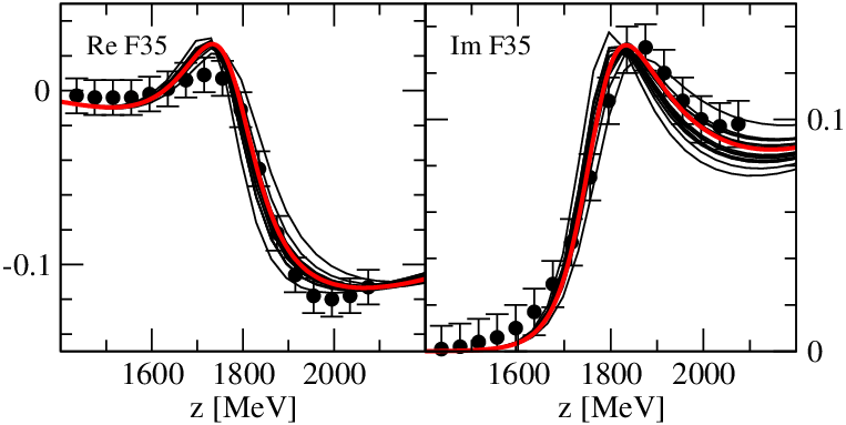


As mentioned in Sec. 3.1, 40 parameters tied to the resonances have been varied to minimize the . There are also other parameters tied to the non-resonant part, given by the form factors shown in Table 7. The latter have been roughly adjusted by hand before carrying out the numerical fit of the resonance parameters, and we do not consider them as free parameters for the error analysis carried out in the following. In the space of 40 parameters the error of parameter is determined by the range of for which the best rises by less than , optimizing at the same time all other 39 parameters. In the limit , this non-linear parameter error approaches the usual parabolic error that can be obtained, e.g., from the Hesse matrix.
Here, we consider only the example of the F35 partial wave. We restrict the determination of the error to the 5-parameter subspace tied to the F35 resonance, e.g., its bare mass [cf. Eq. (4)] and four couplings to the channels , , , and [cf. Eq. (3), B]. Furthermore, we determine the parameter errors within this subspace. This means that in the optimization involved in the determination of the parameter error (see above), only the 4 parameters of the subspace are varied while leaving the other 35 at the optimum. We have checked that this restriction has surprisingly little influence on the parameter error because partial waves are explicitly included in the fit instead of observables; for example, varying a resonance parameter of the P33 partial wave influences a parameter error of the F35 partial wave only indirectly through the inclusion of the data in the total .
The non-linear parameter errors are shown in Table 4.
| [MeV] | ||||
|---|---|---|---|---|
The errors are small for the bare couplings to the and channels, for both of which the data constrain the values. The errors are larger for the bare coupling to the state that is less constrained by data. Indeed, there is a strong correlation between the bare coupling and the bare mass, which therefore also has quite a large parameter error. Although no data are included for the channel, the corresponding bare coupling has small errors. This is because the channel provides most of the phase space that is responsible for the inelastic resonance width, which is well constrained by the elastic amplitude as shown in Fig. 14 to the left.
From the non-linear parameter errors, one can determine the uncertainties of derived quantities such as pole positions, residues, branching ratios, or the amplitude itself. To scan the parameter space within the errors, we have taken four sample points of a given parameter within its error (always optimizing all other parameters). As there are five parameters in the considered subspace, 20 solutions are obtained from which the F35 amplitude and the pole position and residues have been calculated [see Fig. 14 and Table 5]. The error on these quantities is then given by the maximal range reached by these solutions.
| Re [MeV] | [MeV] | |||
| Im [MeV] | [0] |
In Fig. 14, we show also that there are correlations between real and imaginary part of the pole position and also between the branching ratios. As mentioned before, the transition branching ratio is indeed better determined than the individual branching ratio into ; we obtain .
Note that the F35 amplitudes allowed by the discussed criterion, shown in Fig. 14 to the left, lead to a much larger rise in the of the data alone, as an inspection by eye shows. Still, these solutions fulfill the criterion due to the contribution from the data to the total . If one determines, e.g., the uncertainty of the pole position or branching ratio from data alone, one would obtain, of course, much smaller errors on these quantities. Thus, the uncertainties on pole position and branching ratio shown in Fig. 14 and Table 5 should be understood as upper limits.
In summary, we have outlined how to determine the statistical errors of the present results, for the example of the F35 resonance. A rigorous statistical analysis, as outlined above and carried out in Ref. [82] for scattering, requires a direct fit to observables and the full inclusion of , and data and will be carried out in the future, but the present discussion serves to illustrate the error one expects from such an analysis.
6 Summary
A first combined analysis of the reactions and within the unitary dynamical coupled-channels framework has been presented. For the reaction, the world data set from threshold to GeV has been considered.
Dynamical coupled-channels models are particularly suited for combined data analyses: the SU(3) flavor symmetry for the exchange processes allows to relate different final states. The - and -channel diagrams connect also different partial waves and the respective backgrounds.
As a result, for both and , a realistic and structured background can be provided, depending only on a few free constants and form factors whose values are all in a natural range. Consequently, only a minimal set of bare -channel resonances is needed to obtain a good fit to the combined data sets. This may also be tied to the fact that in this field-theoretical, Lagrangian based approach, the dispersive parts from intermediate states are fully included and thus, analyticity is ensured.
Apart from the well-established 4-star resonances, a wide state has been found, dynamically generated from the unitarization of the - and -channel exchanges. Furthermore, there is a clear need for the three-star resonance. This state is found to couple only weakly to but stronger to . Thus, in the present combined analysis of elastic scattering and production, evidence for a “missing resonance state” [8] could be accumulated which indeed has no clear signal in elastic scattering alone.
Acknowledgement
The work of M.D. is supported by DFG (Deutsche Forschungsgemeinschaft, GZ: DO 1302/1-2). This work is supported in part by the Helmholtz Association through funds provided to the virtual institute “Spin and Strong QCD” (VH-VI-231), by the EU-Research Infrastructure Integrating Activity “Study of Strongly Interacting Matter" (HadronPhysics2, grant n. 227431) under the Seventh Framework Program of EU and by the DFG (TR 16). F.H. is grateful to the COSY FFE grant No. 41788390 (COSY-058).
Appendix A Exchange potentials with KY states
In A.1 we list the explicit expressions for the - and -channel exchange diagrams that involve the and channels. For the other exchange processes contained in the model, see Ref. [40]. The new coupling constants for the exchange processes with participation are related to the cases without through SU(3) symmetry. The corresponding expressions can be found in A.2.
The kinematical quantities are specified in Fig. 15. The index and ( and ) denote the incoming and outgoing baryon (meson). The on-shell energies are
| (19) |
for the baryon and the meson, respectively. In the TOPT framework used in this study, the zeroth component of the initial and final momenta are set to their on-mass-shell values: or .


is the three-momentum of the intermediate particle. with (baryon exchange) or (meson exchange) means the 4-momentum in the first time ordering whereas indicates the second time ordering with (baryon exchange) or (meson exchange). Furthermore, in the potentials quoted in A.1, is the Rarita-Schwinger propagator of spin particles given in Ref. [39], and .
If the intermediate particle is a baryon, we use [83] with
| (20) |
Each exchange diagram includes a kinematical normalization factor
| (21) |
The isospin factors for the exchange processes without the participation of the channels can be found in Refs. [39, 40]. For the extension to the channels, carried out in the present work, the isospin factors can be found in Table 6. Also, every exchange process quoted in A.1 is multiplied with form factors corresponding to the two vertices, quoted in A.2.
| Transition | Exchange | IF | IF | Transition | Exchange | IF | IF |
|---|---|---|---|---|---|---|---|
| ex. | ex. | 0 | |||||
| ex. | ex. | 0 | |||||
| ex. | ex. | 0 | |||||
| ex. | ex. | ||||||
| ex. | ex. | ||||||
| ex. | ex. | ||||||
| ex. | ex. | ||||||
| ex. |
A.1 Amplitudes for the exchange diagrams with
The following expressions give the amplitudes shown in Fig. 1 in the helicity base,
| (22) |
with the notation for the momenta as in Fig. 15 and the dependence of the amplitude is on the c.m. (off-shell) three-momentum of the incoming (outgoing) meson-baryon system, , and the total scattering energy . To solve the scattering equation in the -basis, these expressions still have to be partial wave projected [38, 39, 40].
- 1.
-exchange
- 1.
-exchange
- 1.
-exchange
- 1.
-exchange
- 1.
-exchange
- 1.
-exchange
- 1.
-exchange
- 1.
-exchange
- 1.
-exchange
- 1.
-exchange
- 1.
-exchange
- 1.
-exchange
- 1.
-exchange
- 1.
-exchange
- 1.
-exchange
A.2 Coupling constants, form factors (-, -exchanges)
First, the coupling constants needed for the exchange diagrams (Fig. 1, expressions in A.1) are quoted, followed by the form factors and their values.
The coupling constants are related to their counterparts without strange particles by SU(3) flavor symmetry [84] as outlined in Sec. 2.3. The coupling of baryon octets and pseudoscalar meson octet depends on two parameters corresponding to the symmetric and antisymmetric octet. They can be related to the coupling constant and the mixing parameter in the notation of Ref. [84], which is also used here,
| (23) |
and can be also expressed in terms of the standard and couplings [61]:
| (24) |
with (definition of of Ref. [84]). The couplings of the physical and are obtained assuming ideal mixing of the SU(3) states , , i.e., the meson does not couple to the nucleon (see, e.g., Ref. [61]).
Within SU(3), the mixing angle is a free parameter but can be determined from SU(6). We use [85] (The index denotes a pseudoscalar meson and means a vector meson)
| (25) |
For the coupling of vector mesons to octet baryons we use the following Lagrangian:
| (26) |
which consists of a vector part with and a tensor part with . The three fields , and are connected through a vector coupling and a tensor coupling [86, 87]. The SU(3) couplings quoted below are therefore divided into a vector part and a tensor part. We use [85] and .
The coupling of the and the to the meson was not fixed by SU(3) symmetry since the is not a stable particle but regarded as an effective meson-meson state [38, 39, 40], i.e. as a correlated exchange process. In the calculation for the background diagrams we take the following values from [49, 86], obtained from the hyperon nucleon interaction:
| (27) |
The coupling was set to a different value compared to [49, 86]. We choose . The SU(3) symmetric coupling constants are given by the following expressions:
- 1.
Couplings for octet baryon, octet baryon and pseudoscalar meson:
(28) - 2.
Vector coupling for octet baryon, octet baryon and vector meson:
(29) - 3.
Tensor coupling for octet baryon, octet baryon and vector meson:
(30) - 4.
Coupling for pseudoscalar meson, pseudoscalar meson and vector meson:
(31) - 5.
Coupling for decuplet baryon, octet baryon and pseudoscalar meson:
(32)
For the new diagrams of Fig. 1, we use the same expressions for the form factors as in Ref. [40],
| (33) |
where is the mass and the momentum of the exchanged particle. denotes a monopole or dipole form factor. The dipole type applies to vertices with , , or as exchanged particle, otherwise a monopole form factor is used. For the form factors of all other exchange diagrams of the model, see Ref. [40]. The numerical values for the new form factors are given in Table 7.
| Vertex | Ex | [MeV] | Vertex | Ex | [MeV] |
|---|---|---|---|---|---|
The numerical values for the other diagrams (without ) have not been changed, see Ref. [40] for the values.
Appendix B Bare resonance vertices
The bare resonance vertices for are given by the effective Lagrangians listed in Table 8. There, for the field of the meson. The vertices derived from these Lagrangians are partial wave projected to the -basis [39, 40].
The Lagrangians for the couplings have the same structure as for the couplings, the ones for the couplings have the same structure like for the case except for the replacements , , or . Thus, they are not quoted explicitly in Table 8.
| Vertex | Vertex | ||
|---|---|---|---|
Additionally, form factors are supplied for each vertex, given by
| (34) |
where is the nominal mass of the resonance () and , denote the on-shell energies of the incoming or outgoing baryon and meson with c.m. (off-shell) momentum . We have in the case of for all channels except for (). For we have for all channels except for (). For the cut-off parameter we choose GeV, except for the resonance, where we fine-tune GeV for the vertices to the , states, respectively.
| [MeV] | |||||
|---|---|---|---|---|---|
In B.1 we list the partial wave projected, bare resonance annihilation vertices . The bare coupling constants obtained in the fit can be found in Table 9. Every vertex function is multiplied with the corresponding form factor of Eq. (34) and the isospin factor listed in Table 10,
| (35) |
with from Eq. (3). The resonance creation vertices are given by . In Eq. (35) and B.1, and denote the baryon and meson on-shell c.m. energies, respectively, is the baryon mass of the channel, and is the baryon-meson c.m. momentum.
As mentioned in Sec. 2.2, the resonance vertices with total spin have not been derived from Lagrangians. Instead, they have been constructed obeying the correct dependence on the orbital angular momentum (centrifugal barrier). From parity considerations, one can easily relate the bare vertices from the resonances with to those of higher spin,
| (36) |
with the from Eq. (35). Eq. (36) provides the correct dependence on for all channels , , , and .
B.1 Partial wave projected resonance vertex functions
In the following, the classification of vertices corresponds to the quantum numbers of the channel. E.g., refers to the resonances that couple to in -wave, as for example the or . The other channels can, of course, couple with different orbital momentum and (note there are three and two channels with different combinations of and ).
In all cases, the vertex functions for the resonance couplings to and are the same as for the case except for the different masses and isospin coefficients from Table 10. Thus, the vertices are not quoted explicitly.
- 1.
- 2.
(L=0, S=1/2)
- 3.
(L=2, S=3/2)
- 4.
- 1.
- 2.
(L=1, S=1/2)
- 3.
(L=1, S=3/2)
- 4.
- 1.
- 2.
(L=1, S=1/2)
- 3.
(L=1, S=3/2)
- 4.
(L=3, S=3/2)
- 5.
(L=1)
- 6.
(L=3)
- 1.
- 2.
(L=0, S=3/2)
- 3.
(L=2, S=1/2)
- 4.
(L=2, S=3/2)
- 5.
(L=0)
- 6.
(L=2)
Appendix C Residues and branching ratios
The residue and constant term from the Laurent expansion of Eq. (5) can be obtained by a closed contour integration along a path around the pole position ,
| (37) |
Alternatively, the residue and subsequent terms in the Laurent expansion can be obtained by an iterative procedure according to
which is numerically stable (the inverse matrix has a simple zero at ) and fast (no integration required).
The residue and constant term, and , can be expressed in terms of dressed quantities [55],
| (39) |
where (, ) is the dressed annihilation vertex (creation vertex, self-energy) as defined in Eq. (3), evaluated on the second sheet at . Eq. (39) shows that there is a contribution to the constant term from , as expected, but also from the pole term. This is one of the reasons why an identification of as background is problematic [55].
For the two-resonance case shown in Eq. (4), the residues can be expressed in terms of dressed quantities like in the one-resonance case of Eq. (39),
| (40) |
where is the residue of resonance with pole at .
Using Eqs. (6) and (5), the pole residues as quoted by the PDG [61] can be calculated. For the residue phase [61] we consider the usual [13, 14] definition given by
| (41) |
for a resonance with width on top of a background . Comparing Eq. (41) with Eq. (5) and using Eq. (6), the pole residue and its phase are given by
| (42) |
where is the phase space factor from Eq. (6) for the transition, evaluated at the complex pole position. For the corresponding quantity in the reaction , one simply replaces .
It is convenient to express the different residues [with for the transitions within channels] in terms of parameters . Indeed, the residues factorize with respect to the channel space and, e.g., for the residues into the and channels,
| (43) |
with a unique set of up to one undetermined global sign. For the channels and , the partial decay widths are evaluated using
| (44) |
with the resonance mass (final baryon, final meson mass) () and , are the meson and nucleon energy at the on-shell momentum .
The sum of partial decay widths should equal the total width, . The right-hand side of this equation can be determined independently () and be used as a test of the formalism. Indeed, below the threshold, the equality holds to the 1 % level (The definition of branching ratios into the effective states , , is model-dependent anyways). Although Eq. (44) is a good approximation to the partial decay widths, it should be noted that never holds exactly, even in a manifestly unitary coupled-channels model with only stable intermediate states. This is simply because the amplitude has non-analytic branch points, required by unitarity, and this information is not contained in the . However, this does not become a real issue unless a pole is very close to a branch point.
References
- [1] S. Dürr et al., Science 322, 1224 (2008).
- [2] J. J. Dudek, R. G. Edwards, M. J. Peardon, D. G. Richards and C. E. Thomas, Phys. Rev. Lett. 103, 262001 (2009).
- [3] J. Bulava et al., Phys. Rev. D 82, 014507 (2010).
- [4] G. P. Engel, C. B. Lang, M. Limmer, D. Mohler and A. Schäfer [BGR [Bern- Graz-Regensburg] Collaboration], Phys. Rev. D 82, 034505 (2010).
- [5] N. Isgur and G. Karl, Phys. Rev. D 18, 4187 (1978).
- [6] S. Capstick and N. Isgur, Phys. Rev. D 34, 2809 (1986).
- [7] U. Löring, B. C. Metsch and H. R. Petry, Eur. Phys. J. A 10, 395 (2001).
- [8] R. Koniuk and N. Isgur, Phys. Rev. Lett. 44, 845 (1980).
- [9] E. Klempt and J. M. Richard, Rev. Mod. Phys. 82, 1095 (2010).
- [10] D. J. Candlin et al., Nucl. Phys. B 226, 1 (1983).
- [11] D. J. Candlin et al. [Edinburgh-Rutherford-Westfield Collaboration], Nucl. Phys. B 238, 477 (1984).
- [12] R. Cutkosky et al., Proc. of the 1980 Toronto Conf. on Baryon Resonances, p.19.
- [13] G. Höhler et al., Handbook of pion-nucleon scattering, Physik Daten, Vol.12-1, (1979).
- [14] G. Höhler, Newsletter 9, 1 (1993).
- [15] D. J. Candlin et al., Nucl. Phys. B 311, 613 (1989).
- [16] Yu. Valdau et al., Phys. Rev. C 81, 045208 (2010).
- [17] S. Abd El-Samad et al. [TOF Collaboration], Phys. Lett. B 688, 142 (2010).
- [18] A. Gasparyan, J. Haidenbauer, C. Hanhart and J. Speth, Phys. Rev. C 69, 034006 (2004).
- [19] K. Tsushima, S. W. Huang and A. Fäßler, Phys. Lett. B 337, 245 (1994).
- [20] G. Penner and U. Mosel, Phys. Rev. C 66, 055211 (2002).
- [21] G. Penner and U. Mosel, Phys. Rev. C 66, 055212 (2002).
- [22] V. Shklyar, G. Penner and U. Mosel, Eur. Phys. J. A 21, 445 (2004).
- [23] V. Shklyar, H. Lenske and U. Mosel, Phys. Rev. C 82, 015203 (2010).
- [24] D. M. Manley and E. M. Saleski, Phys. Rev. D 45, 4002 (1992).
- [25] O. Scholten, A. Y. Korchin, V. Pascalutsa and D. Van Neck, Phys. Lett. B 384, 13 (1996).
- [26] A. Anisovich, E. Klempt, A. Sarantsev and U. Thoma, Eur. Phys. J. A 24, 111 (2005).
- [27] A. V. Sarantsev, V. A. Nikonov, A. V. Anisovich, E. Klempt and U. Thoma, Eur. Phys. J. A 25, 441 (2005).
- [28] A. V. Anisovich, E. Klempt, V. A. Nikonov, A. V. Sarantsev and U. Thoma, arXiv:1009.4803 [hep-ph].
- [29] R. A. Arndt, I. I. Strakovsky, R. L. Workman and M. M. Pavan, Phys. Rev. C 52, 2120 (1995).
- [30] R. A. Arndt, W. J. Briscoe, I. I. Strakovsky, R. L. Workman and M. M. Pavan, Phys. Rev. C 69, 035213 (2004).
- [31] R. A. Arndt, W. J. Briscoe, I. I. Strakovsky and R. L. Workman, Phys. Rev. C 74, 045205 (2006).
- [32] R. L. Workman, R. A. Arndt and M. W. Paris, Phys. Rev. C 79, 038201 (2009).
- [33] M. Batinić, I. Šlaus, A. Švarc and B. M. K. Nefkens, Phys. Rev. C 51, 2310 (1995), [Erratum-ibid. C 57, 1004 (1998)].
- [34] T. P. Vrana, S. A. Dytman and T. S. H. Lee, Phys. Rept. 328, 181 (2000).
- [35] S. Ceci, A. Švarc and B. Zauner, Eur. Phys. J. C 58, 47 (2008).
- [36] Y. Surya and F. Gross, Phys. Rev. C 53, 2422 (1996).
- [37] U.-G. Meißner and J. A. Oller, Nucl. Phys. A 673, 311 (2000).
- [38] C. Schütz, J. Haidenbauer, J. Speth and J. W. Durso, Phys. Rev. C 57, 1464 (1998).
- [39] O. Krehl, C. Hanhart, S. Krewald and J. Speth, Phys. Rev. C 62, 025207 (2000).
- [40] A. M. Gasparyan, J. Haidenbauer, C. Hanhart and J. Speth, Phys. Rev. C 68, 045207 (2003).
- [41] M. Döring, C. Hanhart, F. Huang, S. Krewald and U.-G. Meißner, Nucl. Phys. A 829, 170 (2009).
- [42] A. Matsuyama, T. Sato and T. S. Lee, Phys. Rept. 439, 193 (2007).
- [43] G. Y. Chen, S. S. Kamalov, S. N. Yang, D. Drechsel and L. Tiator, Phys. Rev. C 76, 035206 (2007).
- [44] N. Suzuki, T. Sato and T. S. Lee, Phys. Rev. C 79, 025205 (2009).
- [45] J. W. Wagenaar and T. A. Rijken, Phys. Rev. C 80, 055205 (2009).
- [46] N. Fettes, U.-G. Meißner and S. Steininger, Nucl. Phys. A 640, 199 (1998).
- [47] N. Fettes and U.-G. Meißner, Nucl. Phys. A 693, 693 (2001).
- [48] A. Gasparyan and M. F. M. Lutz, Nucl. Phys. A 848, 126 (2010).
- [49] A. Müller- Groeling, K. Holinde and J. Speth, Nucl. Phys. A 513, 557 (1990).
- [50] R. Aaron, R. D. Almado and J. E. Young, Phys. Rev. 174, 2022 (1968).
- [51] O. Krehl, C. Hanhart, S. Krewald and J. Speth, Phys. Rev. C 60, 055206 (1999).
- [52] J. Wess and B. Zumino, Phys. Rev. 163, 1727 (1967).
- [53] U.-G. Meißner, Phys. Rept. 161, 213 (1988).
- [54] I. R. Afnan and B. Blankleider, Phys. Rev. C 22, 1638 (1980).
- [55] M. Döring, C. Hanhart, F. Huang, S. Krewald and U.-G. Meißner, Phys. Lett. B 681, 26 (2009).
- [56] M. F. M. Lutz and E. E. Kolomeitsev, Nucl. Phys. A 700, 193 (2002).
- [57] M. Döring and K. Nakayama, Eur. Phys. J. A 43, 83 (2010).
- [58]
L. Tiator, S. S. Kamalov, S. Ceci, G. Y. Chen, D. Drechsel, A. Švarc and S. N. Yang,
Phys. Rev. C 82, 055203 (2010). - [59] E. Oset and A. Ramos, Eur. Phys. J. A 44, 445 (2010).
- [60] M. F. M. Lutz, G. Wolf and B. Friman, Nucl. Phys. A 706, 431 (2002) [Erratum-ibid. A 765, 431 (2006)].
- [61] K. Nakamura et al., Journal of Physics G 37, 075021 (2010).
- [62] N. Suzuki, B. Juliá Díaz, H. Kamano, T. S. Lee, A. Matsuyama and T. Sato, Phys. Rev. Lett. 104, 042302 (2010).
- [63] C. J. Joachain, Quantum Collision Theory (North Holland, Amsterdam, 1975).
- [64] L. Wolfenstein, Ann. Rev. Nucl. Part. Sci. 6, 43 (1956).
- [65] M. Winik, S. Toaff, D. Revel, J. Goldberg and L. Berny, Nucl. Phys. B 128, 66 (1977).
- [66] N. L. Carayannopoulos et al., Phys. Rev. B433, 433 (1965).
- [67] C. Baltay et al., Rev. Mod. Phys. 33, 374 (1961).
- [68] F. S. Crawford, F. Grard and G. A. Smith, Phys. Rev. 128, 368 (1962).
- [69] E. H. Bellamy et al., Phys. Lett. B 39, 299 (1972).
- [70] P. Livanos, J. P. Baton, C. Coutures, C. Kochowski and M. Neveu, Contribution presented at 4th Int. Conf. on Baryon Resonances, Toronto, Canada, Jul 14-16, 1980. Published in Baryon 1980:35.
- [71] J. Haba et al., Nucl. Phys. B 299, 627 (1988).
- [72] F. Huang, A. Sibirtsev, S. Krewald, C. Hanhart, J. Haidenbauer and U.-G. Meißner, Eur. Phys. J. A 40 (2009) 77.
- [73]
A. Sibirtsev, J. Haidenbauer, S. Krewald, T. S. H. Lee,
U.-G. Meißner and A. W. Thomas, Eur. Phys. J. A 34 (2007) 49. - [74] A. Baldini, V. Flamino, W. G. Moorhead, and D. R. O. Morrison, Total Cross Sections of High Energy Particles: Landolt-Börnstein, Numerical Data and Functional Relationships in Science and Technology, edited by H. Schopper (Springer- Verlag, New York, 1988), Vol. 12a.
- [75] M. Döring, E. Oset and U.-G. Meißner, Eur. Phys. J. A 46, 315 (2010).
- [76] B. Juliá Díaz, T. S. Lee, A. Matsuyama and T. Sato, Phys. Rev. C 76, 065201 (2007).
- [77] S. Capstick and W. Roberts, Phys. Rev. D 47, 1994 (1993).
- [78] S. Capstick and W. Roberts, Phys. Rev. D 49, 4570 (1994).
- [79] G. Ramalho and K. Tsushima, Phys. Rev. D 82, 073007 (2010).
- [80] S. R. Deans, R. W. Mitchell, D. L. Montgomery, G. C. Wood and J. E. Rush, Nucl. Phys. B 96, 90 (1975).
- [81] K. Nakayama, Y. Oh and H. Haberzettl, arXiv:0803.3169 [hep-ph].
- [82] B. Borasoy, U.-G. Meißner and R. Nißler, Phys. Rev. C 74, 055201 (2006).
- [83] C. Schütz, K. Holinde, J. Speth, B. C. Pearce and J. W. Durso, Phys. Rev. C 51, 1374 (1995).
- [84] J. J. de Swart, Rev. Mod. Phys. 35, 916 (1963) [Erratum-ibid. 37, 326 (1965)].
- [85] G. Janßen, K. Holinde and J. Speth, Phys. Rev. C 54, 2218 (1996).
- [86] B. Holzenkamp, K. Holinde and J. Speth, Nucl. Phys. A 500, 485 (1989).
- [87] A. Reuber, K. Holinde and J. Speth, Nucl. Phys. A 570, 543 (1994).