The cavity method for quantum disordered systems: from transverse random field ferromagnets to directed polymers in random media
Abstract
After reviewing the basics of the cavity method in classical systems, we show how its quantum version, with some appropriate approximation scheme, can be used to study a system of spins with random ferromagnetic interactions and a random transverse field. The quantum cavity equations describing the ferromagnetic-paramagnetic phase transition can be transformed into the well-known problem of a classical directed polymer in a random medium. The glass transition of this polymer problem translates into the existence of a ‘Griffiths phase’ close to the quantum phase transition of the quantum spin problem, where the physics is dominated by rare events. The physical behaviour of random transverse field ferromagnets on the Bethe lattice is found to be very similar to the one found in finite dimensional systems, and the quantum cavity method gets back the known exact results of the one-dimensional problem.
I Introduction
The cavity method has been developed to study classical frustrated spin systems: spin glasses. In recent years its range of application has broadened a lot as it was applied with some success to hard computer science problems and also to some quantum problems. This paper aims at giving some background on the cavity method, both classical and quantum, and explaining how it can be used to study a quantum problem, a ferromagnetic spin system in a random transverse field, following the recent work of [[1, 2]]. This is a problem which has been studied a lot in one dimension; we analyze it here using the cavity method which is a mean-field type method better suited for large dimensional systems. However we find that the physics is rather similar to the one found in the one-dimensional case, in the sense that rare events (rare sites with anomalously small transverse fields) play a major role in the neighborhood of the quantum critical point. This leads to very large spatial fluctuations of the spontaneous magnetization in the ferromagnetic phase, and a broad distribution of the local magnetic susceptibilities in the paramagnetic phase. These effects, which are typical of the ‘Griffiths phase’ described in low dimensions, are found here through the use of an auxiliary problem of directed polymers in random media: the rare-event dominated regime of the ferromagnetic-paramagnetic phase transition is related to the glass transition of the polymer problem.
This paper is organized as follows. Sec.II gives an introduction to the cavity method in classical spin systems. Sec.III defines the random transverse field ferromagnet and gives some background on this problem. The naive mean field approach to this problem is explained in Sec.IV. Sec. V introduces the quantum cavity method and discusses some systematic approximation schemes which can be used in this context. These approximation schemes are tested in Sec.VI by applying them to a very simple, and very well understood, problem: the pure ferromagnet in a transverse field. Sec.VII describes the use of the quantum cavity method, with a ‘cavity-mean-field’ approximation, to study the phase diagram of a ferromagnet in a random transverse field. It derives the phase transition line in the plane disorder-temperature, and describes the main properties of the low-temperature ferromagnetic and paramagnetic phases, in particular the large fluctuations of the order parameter and of the susceptibility. This section ends by a study of the one-dimensional case, where the cavity method gets the known exact results, and a discussion of the higher-dimensional cases, for which the Bethe lattice analysis provides a useful mean-field approximation. A short summary is given in Sec.VIII.
II The classical cavity method
II.1 The Sherrington-Kirkpatrick model
The cavity method has been introduced twenty five years ago in the context of spin glass mean field theory [3]. The solution of the fully connected Sherrington-Kirkpatrick (SK) [4] model had been found a few years before by G. Parisi [5], who had proposed, within the replica approach, an inspired Ansatz of replica symmetry breaking (RSB). The cavity method gave an alternative solution, with identical physical content and results to the replica approach, but which was much more transparent. Instead of the mysterious replicas, it used a purely probabilistic approach, based on three assumptions which had been found to be hidden in the form of Parisi’s RSB Ansatz: the existence of many pure states [6], ultrametricity [7], and the exponential distribution of free energies of the pure states [8]. This approach has turned out to be very powerful and has served as a starting point of recent works by Talagrand [9] and Guerra [10] which established rigorously the exactness of the free energy obtained by the RSB/cavity method (although the ultrametric property has still not be proven).
In a nutshell, the cavity method as it was applied to the SK model consists in assuming some structure for a -spin system , and checking self consistently that this structure is reproduced when one adds a new spin and goes to a spin-system. Within the simplest replica symmetric (RS) approximation, the main assumption is that the correlation functions are small. The local field on then has a Gaussian distribution, with a width which must be reproduced self-consistently and gives the Edwards-Anderson order parameter [11]. This approach gives the RS solution, which is correct at temperatures above the de-Almeida Thouless (AT) line [12]. It breaks down in the spin glass phase, when the proliferation of pure states induces a non-trivial correlation between distinct spins. In order to study the spin glass phase, one must explicitly assume the existence of many pure states [13, 14] with free energies distributed as a Poisson process with exponential distribution [3]. Within each state, the correlations are small and the cavity method can be applied. But the addition of the new spin creates a free energy shift which depends on the state: the free energies are reshuffled, and the selection of low free energy states (by the Boltzmann weight) biases the local field distribution. The whole cavity RSB approach relies on controlling these crossings of the free energies of the states, and checking the self consistency of the basic hypotheses. The results are exactly identical to those of the replica approach.
II.2 Finite connectivity spin glasses
It was soon realized that it would be very instructive to go beyond the SK model by studying spin glass models in which each spin has only a finite number of neighbours. In order to introduce mean field models with this property, the usual approach is to study the Bethe lattice, which is usually defined as the interior of a Cayley tree: taking a large Cayley tree of depth , one studies the interior part up to depth . The Bethe lattice is then defined by the double limit (see Fig. 1). This procedure is fine for ferromagnetic interactions, but it raises a problem when one studies spin glasses where a crucial ingredient is the frustration due to loops in which the product of exchange couplings is negative. A simple procedure is to induce frustration by fixing randomly (or imposing some type of local fields on) the spins at the boundary of the tree. However most of the physics is then put by hand through this boundary condition, which involves a finite fraction of the total number of spins. For instance fixing the boundary spins to independently with probability 1/2 [15, 16] gives a system which does not have a genuine spin glass phase (technically it is is always replica symmetric). It has been found recently how the boundary conditions should be fixed in order to get RSB: the correct procedure involves the process of broadcast and reconstruction [17] and creates subtly correlated boundary fields.


An alternative construction is to define the Bethe lattice spin glass through a random regular graph, taken uniformly from all the graphs where each spin has neighbours (see Fig. 1). Large random regular graphs with vertices have a locally tree-like structure like the interior of a Cayley tree, as the typical size of a loop is of order . These large loops create the frustration without having to play with boundary conditions. The study of spin glasses on random graph with a finite connectivity started with Viana and Bray [18]. The solution of spin glasses on random regular graphs within the RS approximation was found relatively early [18, 19, 20], but it took fifteen more years to understand how to handle RSB effects [21], and this has been done so far only at the level of one, or at most two, steps of RSB. Here we shall briefly review how the cavity method can be used to study this problem, mostly at the RS level, as this gives the building blocks of the quantum cavity method which we use below.
Let us study the equilibrium properties, at inverse temperature , of a general Ising spin glass problem with a random field on a Bethe lattice, defined by the Hamiltonian
| (1) |
where are the links of a random-regular graph of degree . The idea is to use the local tree-like property for rooted trees. Let us pick up one spin, say , and delete the edge between and one of its neighbours. Up to any finite distance, is now the root of a tree. Let us denote by the local ’cavity’ magnetic field on the root due to this tree, so that . Denote by its neighbours on the tree, and by their cavity fields (so that for instance the magnetization of in the absence of is ). The Boltzmann measure on is then
| (2) |
By doing explicitely the sum over the spins , one gets the recursion
| (3) |
which is illustrated pictorially in Fig.2. One way to describe it is to build the tree rooted in by considering the trees rooted on (in absence of ) and merging them.
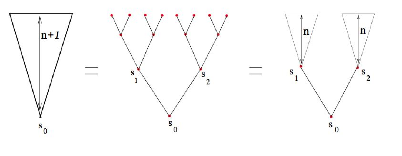
These recursion ‘cavity’ equations are always correct on a tree. On a random regular graph they are correct whenever the joint probability of the spins in the absence of factorizes into a product . Two conditions are needed for this absence of correlations of neighbouring spins. One is the local tree-like property which guarantees that any two neighbouring spins , with , are far away on the graph obtained by eliminating the site and all edges connected to it. The second one is that the correlations decay at large distance, so that the correlations between two neighbours and (which are typically at distance when is absent), vanish in the large limit. This is true when the system is in its paramagnetic phase. It is not correct in a ferromagnetic phase or in a spin glass phase because long-range correlations develop. However, if one is able to restrict the measure to one single pure state (where by definition correlations decay at large distance), then the recursion relations are correct.
These recursion relations can be used in two main ways:
1- On a given sample, one can see these equations as a set of self-consistent equations relating cavity fields: there are two such cavity fields for each edge of the graph, one is the field on site in the absence of (case where has been chosen as root), the other one is the field on site in absence of . All these fields are related by the cavity equations. In the large limit these equations reduce to the ’TAP’ equations [13]. These RS cavity equations are also well known in computer science under the name of ‘belief propagation’ equations [22].
2- One can also study the statistics of cavity fields. Suppose that the local magnetic fields are independent random variables drawn from a distribution , and the exchange couplings are independent random variables drawn from a distribution . At the RS level, one expects a single solution for all cavity fields on a given instance. Then one can define the distribution of cavity fields when one picks up an oriented edge randomly. This is the natural order parameter for this problem. Its knowledge provides the full solution of the problem when the RS hypothesis is correct. Technically, finding is usually done by a ‘population dynamics’ method first introduced in [[23]], and developed in the present context by [[21]]. Its idea is the following. The update equation (3) induces a self-consistency equation for which can be written as:
| (4) |
The population dynamics method represents by a population of fields . This population is updated by a Monte-Carlo-type process in which, at each iteration, one does the following operations:
- •
Choose indices randomly uniformly.
- •
Generate independent couplings from , and a field from .
- •
Compute
- •
Choose an index randomly uniformly, and replace in the population the value by the new value .
The convergence of this method when the number of iterations is large enough can be checked by monitoring for instance moments of (the -th moment is evaluated as ). If is large enough the population will give a good approximation of .
Note that the RSB situation is much more complicated: on a given instance there are many solutions to the system of equations relating the cavity fields. On a given oriented edge (say looking at the cavity field on in absence of ) the cavity field can take many values depending on the solution one takes. Doing the statistics over all solutions defines a distribution of fields on each oriented edge, and the order parameter is the distribution of these distributions when one picks an edge at random. In the following quantum problems we shall use only the RS version.
III Random transverse-field ferromagnets
The problem of ferromagnets in random transverse fields has received a lot of attention in recent years. These systems provide relatively simple examples of disordered systems displaying a quantum phase transition [24]. They are described by the Hamiltonian:
| (5) |
where are Pauli matrices. The exchange couplings are independent ferromagnetic interactions drawn from a distribution which has support on , and the random transverse fields are independent variables drawn from a distribution . The lattice structure is described by the set of pairs which appear in the above sum; we suppose that this lattice is homogeneous, and each spin has exactly neighbours. For definiteness we shall use a model where the distribution of couplings and fields are given by:
| (6) |
where is the Heaviside function. The choice of the width of the distribution fixes the energy scale such that the mean-field critical temperature in absence of disorder has . The Hamiltonian thus depends on a single parameter which measures the degree of disorder.
The one dimensional case, which is intimately related to the two-dimensional classical model of MacCoy and Wu [25], has been solved in great detail by Fisher [26] using the strong disorder Ma-Dasgupta-Hu decimation procedure [27]. This solution has emphasized the importance of Griffiths singularities, which manifest themselves most notably in the fact that the average susceptibility differs from the typical one. The method itself has a broad range of applications [30]. These results have been confirmed numerically [28, 29], and numerical simulations of the same problem in dimension two, both through the strong disorder decimation and through Monte-Carlo simulations, also point to the same kind of physics as in one dimension [31, 32, 33, 34, 35]. Recent results also find the same behaviour in dimension three and higher [36]
Using the method introduced in [[1, 2]], we shall now study the Bethe approximation for the random transverse-field ferromagnet described by (5). We thus assume that the spins are on the vertices of a random regular graph of degree and we want to study the phase diagram of this problem as function of the temperature and the amount of disorder .
IV Mean field
IV.1 Naive mean field
For large one may be tempted to use the mean-field approach, in which is replaced by where is determined self-consistently from the equation . At temperature , the self consistent equation for obtained at is:
| (7) |
At finite temperature there is a transition between a large disorder paramagnetic phase where is the only solution of this equation, to a ferromagnetic phase characterized by a non-zero field, . The critical temperature is given by:
| (8) |
At zero temperature this naive mean field approach predicts that the system is always in its ferromagnetic phase.
While this approach is correct when , its conclusions are qualitatively wrong for any finite .
IV.2 Bethe-Peierls approximation
The naive mean field prediction that the system is always ferromagnetic at zero is wrong; the reason is that the mean field approach does not take into account properly the rare events. Rare sites where the energy can be easily polarized in the direction, and they play a key role in the establishment of the ferromagnetic order. This effect, which has been first discussed qualitatively in [[37]], leads to a zero temperature quantum phase transition to a paramagnetic state at a critical value of disorder . In order to study this quantum transition in details, we shall use the quantum version of the cavity method.
V The quantum cavity method and its projections
V.1 The RS quantum cavity method
Let us study the transverse-field Ising Hamiltonian (5) on a Bethe lattice defined as a random regular graph. The partition function can be expressed with the Suzuki-Trotter representation. Using imaginary time steps, we introduce at each time step a decomposition on the eigenvectors of the operators . This describes the system by the classical time trajectory of each spin, , where , and denotes the eigenvalue of at time . Then
| (9) |
where:
| (10) |
and
This Hamiltonian acts on spin trajectories . Each trajectory can be seen as a variable taking possible values, and defines the interaction of these variables. The crucial point is that this Hamiltonian involves interactions between pairs of trajectories which are neighbours on the Bethe lattice. This is a locally tree-like graph and therefore one can use the cavity method to study it. The RS cavity method for this problem was introduced in [[38]]. It is obtained from the classical cavity method described in Sec.II.2 by using spin trajectories instead of Ising spins. Take a branch of the Bethe lattice rooted on spin , and define the probability distribution of the time-trajectory of this spin as . Define analogously, for each of the spins which are the first neighbors of on the rooted tree, their time trajectory as . Then one can write the mapping that generates, from , the new :
| (11) | |||||
The population dynamics method of Sect.II.2 can be used to study this cavity recursion: one must represent each of the by a sample of spin trajectories. This has been done for some problems in [[38, 39]], but this approach tends to be rather heavy numerically. In particular, in a disordered system like the random transverse-field ferromagnet, the natural order parameter is the distribution of the functions when the site is drawn randomly. This is a rather complicated object which must be represented as a population of populations.
V.2 The projected cavity mapping
While the exact RS cavity mapping is in principle doable, the difficulty in its numerical resolution may make it difficult to get a clear understanding of the physical results. For this reason one may want to develop approximate versions of it. One such approximation, the projected cavity mapping introduced in [[1]], consists in using a local distribution which takes the special form, parameterized by one single number :
| (12) |
Injecting this form into (11) we obtain a which does not have the form (12). However one can project it back on a in the right subspace described by (12) as follows. From the obtained one can compute and deduce from it the effective parameter such that the distribution gives this value of .
This projected cavity mapping is actually more easily understood directly in terms of quantum Hamiltonians, without going to the Suzuki-Trotter formalism. One studies the properties of a spin in the rooted graph where one of its neighbors has been deleted, assuming that the remaining neighbors are uncorrelated. Each of these neighbours, when it is at the root of the subtree obtained by deleting the link to spin , is supposed to be described by a Hamiltonian
| (13) |
The system of spin and its neighbors is thus described by the local Hamiltonian
| (14) |
By diagonalizing this Hamiltonian, one can compute the induced magnetization of spin , . In order for this approach to be self-consistent, this magnetization should be equal to the one obtained from the Hamiltonian . This means that is obtained by solving the equation:
| (15) |
The projected cavity mapping thus uses a single number to describe the trajectory distribution . It leads to a mapping which gives the new cavity field in terms of the fields on the neighboring spins. This mapping induces a self-consistent equation for the distribution of the fields, which is the natural order parameter in this context: the paramagnetic phase has , and the ferromagnetic phase is described by a non-trivial . The population dynamics method can be used to find this distribution.
V.3 The cavity-mean-field approximation
The projected cavity mapping is numerically much simpler than the full RS cavity method using spin trajectories. It also allows to address a broader range of questions, like those related to the real time dynamics and the spin relaxation, which are not easily accessible within the Suzuki-Trotter formalism [1, 2]. Still its practical use is a bit slow numerically as one must diagonalize the spin Hamiltonian (14) each time one wants to generate a new field in the population.
It has turned out useful [1] to use one more step of approximation in order to obtain an explicit mapping, similar to the one found in the classical problem (3). This can be done using a mean field approximation in order to compute the magnetization from the cavity Hamiltonian (14). In this ’ cavity-mean-field approximation ’, one approximates the cavity Hamiltonian acting on spin by
| (16) |
This implies that , giving the explicit recursion equation relating the fields:
| (17) |
This recursion induces a self-consistent equation for the distribution which can now be written explicitly:
| (18) |
VI A simple test of the projected cavity recursion: the pure ferromagnet
It is useful to test the validity of the two levels of approximation described above (the projected cavity mapping and the cavity-mean-field approximation) versus precise results using the full numerical sampling of Suzuki-Trotter trajectories. This can be done in the case of a pure ferromagnet in a uniform transverse field, defined by and . We thus study the problem defined by the Hamiltonian
| (19) |
on a random regular graph where each site has neighbours. The exact cavity study in terms of continuous-time spin trajectories has been done in the case by [[39]], we shall use their results as a benchmark in order to test the accuracy of the three levels of approximations:
1: Naive mean field: The Eq.(7) for the spontaneous field in the direction becomes:
| (20) |
2: Cavity-mean-field: The recursion relation (17) now becomes a self-consistent equation for the spontaneous field in the direction (which is site-independent):
| (21) |
it differs from the naive mean field only by the replacement .
3: Projected cavity mapping: The system of spin and its neighbors is described by the local Hamiltonian
| (22) |
The self-consistent equation for the spontaneous field in the direction is given by
| (23) |
These traces involve matrices of size , they are easily computed numerically when is not too large.
The phase diagram obtained with these three approximations is plotted in Fig.3, and compared to the exact one of [[39]]. The projected cavity mapping gives a rather precise approximation of the phase diagram, much better than the one obtained by naive mean field or by the well known static approximation (see [[39]]). A slightly better result can be obtained by using the parameterized form (12) variationally inside the Bethe free energy [46].
One may also use the cavity method as a mean field approximation to study the finite dimensional problem. It turns out that it is able to locate the transition point rather accurately. For a three dimensional case, the simulations through a cluster Monte-Carlo method of the Suzuki-Trotter formulation [40] gives a zero-temperature transition occuring at . The projected cavity mapping (with ) gives , and the cavity-mean-field gives . In two dimensions, the numerical result of [[32, 40]] is , the projected cavity mapping (with ) gives , and the cavity-mean-field gives .


VII Phase diagram of the random transverse-field ferromagnet
Let us apply the cavity-mean-field approximation to the random transverse-field ferromagnet. The whole problem reduces to finding the distribution of fields which solves the self-consistent equation (18). It turns out that the solution of this equation is more subtle than the one of seemingly similar equations obtained in the classical case.
In order to understand the properties of this solution, it is useful to go back to the cavity mapping (17). Let us iterate this mapping times on the Bethe lattice. For finite and the corresponding graph is just a rooted tree with branching factor at each node and depth . The field at the root is a function of the fields on the boundary. In order to see whether the system develops a spontaneous ferromagnetic order, we study the value of in linear response to infinitesimal fields on the boundary spins. This is given by
| (24) |
where the sum is over all paths going from the root to the boundary, and the product is over all edges along the path .
VII.1 Phase transition and directed polymers
The response is nothing but the partition function for a directed polymer in a random medium (DPRM) on a tree, where there exists on each edge of the tree a random energy given by and the temperature of the polymer has been set equal to one. The random energies are independent identically distributed random variables. We need to compute the large behavior of . As is a partition function, this is naturally characterized by the free energy
| (25) |
If the effect of a small boundary field decays with distance: the spin system is paramagnetic. If it is ferromagnetic.
The general method for computing in DPRM on trees has been developed by Derrida and Spohn [41]. Their solution can be expressed in terms of the convex function
| (26) |
Let us denote by the value of where this function reaches its minimum.The free energy of the DP is then . The phase transition line in the plane separating the ferromagnetic from the paramagnetic phase is thus obtained by solving the equation .
In the case of the random transverse-field ferromagnet one obtains
| (27) |
from which one deduces the following phase diagram (see Fig.4).:
- •
When the field is smaller than a value the phase transition line is given by . This gives back the naive mean field result of (8): . The value , and the corresponding value , are obtained by solving the pair of equations .
- •
When , the phase transition is given by solving the equations . In this regime the solution is at . This low temperature, large disorder part of the phase transition line departs from the naive mean field prediction. In particular, at variance with the naive mean field result, one finds that there exists a zero temperature quantum phase transition at a critical disorder . This is obtained using the zero-temperature limit of :
(28) and solving the two equations . Fig.5 shows as function of . In the large limit diverges, giving back the naive mean field result. However this divergence is very slow: one finds that and .

The phase transition line has two parts: a small-disorder part on the left of the point with coordinates (, and a large-disorder part on the right of this point. The properties of these two regimes of the transition are very different. In order to understand this difference, it is useful to give a closer look at the DPRM problem using the replica method, as was first done in [[42]]. The DP partition function , defined in (24), depends on the random quenched variables . To compute the value of for a typical sample one needs to do a quenched average of over these random variables, denoted by . As a first step one might try to approximate it by the annealed average . This gives precisely the naive-mean field result. To go beyond this ‘annealed approximation’ one can introduce replicas, using . The average of is obtained by a sum over paths,
| (29) |
One can then proceed by testing various hypotheses concerning the structure of the paths which dominate the replicated partition function (29):
- •
In the so-called replica symmetric (RS) hypothesis one assumes that the leading contribution to (29) comes from non-overlapping paths. This gives
(30) The RS hypothesis is equivalent to the annealed approximation in this case.
- •
The so-called one step replica-symmetry-breaking (1RSB) hypothesis assumes that the leading contribution to (29) comes from patterns of paths which consist of groups of identical paths, where the various groups go through distinct edges. This gives:
(31) where is the function introduced in (27). In the replica limit , the parameter should belong to the interval . It turns out that one should minimize the function over (the fact that one should minimize , and not maximize it as one would have thought naively, is a well-known aspect of the replica method [43]). The low-temperature large-disorder part of the phase transition line corresponds to this 1RSB solution.
VII.2 Replica symmetry broken phase of the polymer and Griffiths phase of the ferromagnet
This replica solution of our DPRM, with a RS phase at small disorder and a 1RSB phase at large disorder, fully agrees with the original travelling wave solution of [[41]]. So the point R on the paramagnetic-ferromagnetic transition line of the quantum random transverse-field ferromagnet corresponds to a 1RSB transition in the auxiliary DPRM problem. This is a glass transition of the polymer, similar to the one found in the random energy model [44, 45], where the measure on the paths condenses on a finite number of paths. A useful order parameter to describe this transition is
| (32) |
This is nothing but the sum where is the relative weight of path in the measure (24). Its inverse gives a measure of the effective number of paths contributing to . In the RS phase one finds that vanishes in a typical sample. This can be understood from the fact that the DPRM partition function gets a contribution from a large number of paths (diverging in the large limit). In fact the DPRM problem has a finite entropy in this RS phase. On the contrary, in the 1RSB phase one finds that is finite and fluctuates strongly from sample to sample. For instance, its first moments are given by [[7]]:
| (33) |
and the entropy density of the polymer vanishes in this whole 1RSB phase.
The DPRM problem is an auxiliary construction used to study the phase transition in the original problem of the random transverse field ferromagnet. So the natural question is: what are the consequences of the 1RSB transition in the DPRM concerning the original quantum spin system? Let us go back to (24), which connects the two problems. We consider a large tree of length . The condensation of the paths in the DPRM means that, if a small field is applied to the boundary, the value of the effective field on the root is dominated by a finite number of paths to the boundary. So the root spin feels the effect of only a finite number of the boundary spins. The physics is dominated by rare events: rare boundary spins have a dominant influence of the central spin, and it is building up on these rare events that the system can or cannot develop a long range ferromagnetic order. This is very similar to the Griffiths phase, found originally in the one-dimensional case [26], and argued to be present at least in low-dimensional systems. It is interesting to see that we find here a similar rare-event dominated phase, using the mean-field type Bethe approximation which is valid in the opposite limit of large connectivity, . The next subsections will give a more detailed discussion of the connections between the results obtained with the cavity method and those known, or conjectured, for finite-dimensional problems. Let us first summarize the main observables that are accessible using the cavity method.
One can study the practical consequences effect of the rare events on both sides of the phase transition, in the neighborhood of the phase transition line, on the right of point R. The study of [[2]] has discussed these effects in the context of the superconductor-insulator transition. It is easy to translate them to the present situation of the ferromagnetic-paramagnetic transition.
- •
In the ferromagnetic phase the order parameter (here we use as order parameter the typical local magnetic field in the z direction, obtained as ) has an anomalous scaling and distribution. Imagine one enters the ferromagnetic phase at a given temperature by varying the disorder . At large enough temperature the scaling is , as one expects in a mean field system. Then lowering the temperature there is a region above where the scaling is . The exponent diverges when . In the 1RSB regime, i.e. for , the typical field has an essential singularity in . In this regime the distribution of the local order parameter has a power law tail . As , the average order parameter is divergent.
- •
In the paramagnetic phase the local susceptibility fluctuates strongly from site to site and nonlinear effects are crucial. Consider the system in a very small uniform magnetic field and look at the local order parameters induced by this external field. The typical value of scales linearly with , but the moments with , and in particular the mean , are divergent at the level of the linear response to : they behave non-linearly, as . The distribution of the local susceptibilities has a power law tail .
VII.3 The one-dimensional case
The one-dimensional RTFF is the best understood case. The strong disorder decimation procedure of Ma-Dasgupta-Hu, developed by Fisher [26], becomes exact at the transition point because of the existence of an infinite disorder fixed point. It can also be checked versus alternative methods like the mapping of the problem to free fermions [28, 29], and the exact solution of McCoy and Wu [25]. A large corpus of results has been obtained by these methods, concerning the scaling behaviour and the Griffiths phase. The strong disorder decimation has turned out to be useful in a broad range of problems [30].
Let us mention only some aspects of the physics of the one-dimensional case for which one can draw a comparison between the exact results and those of the cavity method. The exact analysis of the problem has shown that the zero-temperature critical point is located at the width of the random transverse field such that , or explicitely: . In our case this gives . At the critical point the system displays activated dynamical scaling: the scaling exponent , relating the characteristic time scale to the characteristic length scale through , is formally infinite. Instead the scaling is . The Griffiths phase can be studied close to the critical point. Defining , where the overline denotes the average and denotes the variance, this exponent has been shown to behave as , where is a non-universal constant. This exponent also appears in the singular response of the system to an external magnetic field : in the paramagnetic phase, the linear susceptibility diverges, and the magnetization behaves as .
Let us now present the results of the cavity method described in the previous subsection. The one-dimensional case is obtained by taking . Actually it is useful to keep at intermediate steps of the computation, and take the limit in the end. At zero temperature, the minimum of the function is obtained at , and the critical value of , obtained by solving , is . When , goes to which is the exact result, and . The exponent is the one that controls the decay of the local field distribution (which goes as ), and the distribution of local susceptibilities. From the analysis of [[2]], this exponent controls the response to a uniform external field, . So one should identify . At the critical point we have found . This agrees with and the activated scaling behaviour. Let us now study the behaviour close to the critical point, at . At (or ), one obtains . So the prediction of the cavity method is . It turns out that, when expressed in terms of the distance to the critical point , this gives the exact result .
The quantum cavity method is exact in one dimension, if one uses the full mapping of spin trajectories given in (11). It must thus reproduce the exact results. What we have seen is that even the simpler cavity-mean-field approximation gives a fair description of the problem, including the exact location of the critical point, the activated dynamical scaling, and the correct value of close to the critical point. Actually it gives the exact correlation even for a finite length problem, as we now show.
Consider a chain described by the Hamiltonian
| (34) |
In order to see the onset of long-range order, one can fix that the end-spin is in the eigenstate of with eigenvalue , fix , and compute the so-called ’surface’ magnetization at the other end-point in the ground state . By using the Jordan-Wigner transformation of this problem to free fermions, Iglói and Rieger have shown that [29]:
| (35) |
This formula, which is exact for a finite system, can then be used to study the critical behavior of the problem. For instance, [[29]] shows how to deduce from this formula several interesting physical properties: the typical and the average surface magnetization differ, the average critical magnetization scales like , the exponent giving the surface magnetization close to the critical point is equal to , the correlation length exponent exponent is equal to .
Let us now use the cavity-mean-field method on this one-dimensional problem. At zero temperature, formula (17) gives the recursion
| (36) |
which should be initialized with . It is easy to see that, iterating the mapping (36), and computing , one obtains the exact formula (35). Therefore the cavity method, even using the simplified, mean-field mapping, gives the exact value of the surface magnetization, also for a finite system. Its predictions thus agree with the known results, including the values of the exponents and .
VII.4 Dimensions two and above
There is no exact solution of the two-dimensional RTFF problem. This problem has been studied mostly using the strong-disorder decimation procedure [33, 35, 36], and also using cluster Monte-Carlo simulations of the 2+1 dimensional problem obtained in the Suzuki-Trotter representation[31, 32]. These works have mostly used a different normalization, in which is the uniform distribution on , and is uniform on . In this subsection we shall thus adopt this other normalization. The results obtained both by decimation and by Monte-Carlo indicate that the situation is similar to the one-dimensional case. In particular, the exponent is found to diverge, and goes to zero as . In order to obtain an analytic approximation to this two-dimensional problem, one can repeat the cavity study on the Bethe lattice with .
Within the cavity-mean-field approximation, the function is found to be
| (37) |
It is minimum at , and the critical value of the field, obtained from , is found to be . This result disagrees with the strong-disorder decimation, and with the Monte-Carlo, in two aspects: i) the value of (with the Monte-Carlo it is found [31, 32] around , with the decimation it is found [35, 36, 34] around ), ii) most importantly, the fact that the value of found in the cavity method does not go to zero at the transition.
One may wonder to what extent these results depend on the approximation. If instead of doing the cavity-mean-field approximation one uses the more accurate projected cavity mapping, the value of is changed to , but the value of is unchanged. This is seen from Fig.6, which shows the inverse of the typical value of the local field , measured as , plotted versus . The prediction of [[2]] is that the inverse of the typical value of should go to zero linearly in . Both data sets, obtained from the cavity-mean-field approximation and from the projected cavity mapping, find this behaviour, but the values of in both data sets are distinct (respectively , as predicted from our analytic study with the DPRM, and , found from the fit).

The conclusion is that, while the non-universal critical value depends quite a lot of the approximation used in the cavity method, the value of does not, and the statement that at the transition seems to be a solid result for the problem on the Bethe lattice with any connectivity . Notice that this result still implies that there is a strong hierarchy of local magnetic fields: the average field diverges, and so does the average susceptibility. But it is not an infinitely strong hierarchy as happens when . It should be noticed that our best cavity analysis, using projected cavity mapping, still involves some approximation, and it would be interesting to carry out the full Suzuki-Trotter trajectory mapping in order to get the exact solution for the Bethe lattice. At present, our approximate treatment gives at the transition for the Bethe lattice problem a result which disagrees with a recent study from strong disorder decimation [36]. It should be noticed that our cavity approximations shoud become exact in the large limit of the Bethe lattice. Assuimng that the result is correct for the Bethe lattice, this raises the question of the existence and value of a critical dimension above which the finite dimensional problems have .
It would thus be interesting to revisit the numerical results in and , and on the Bethe lattice, giving at the transition. Concerning the Monte-Carlo approach, let us point out in particular that the RSB effects happen at very low temperature, but they completely change the physics of the problem (for the problem with and uniform couplings on , we have found with the cavity-mean-field approximation that the RSB transition point on the ferromagnetic-paramagnetic transition line occurs at ). So the numerical results obtained by extrapolation from a not-very-low temperature to might be questionable.
VIII Summary
We have proposed here a well defined mean-field scheme to study quantum ferromagnets in random transverse fields. This scheme consists in studying the problem on a random regular graph with fixed connectivity . The problem at finite is qualitatively distinct from the infinite case, described by the naive mean field theory. It has a zero temperature quantum phase transition at a finite critical value of the width of the distribution of random transverse fields.
The phase diagram has been studied by the RS quantum cavity method. A full study would involve a complicated population dynamics in terms of imaginary time spin trajectories, which would be extremely costly in terms of computing efforts. Instead we have resorted to a simple approximation, the cavity mean-field approximation, which parameterizes the imaginary time spin trajectories by a single number, a local cavity longitudinal field. Within this approximation, the RS cavity method becomes a simple recursion relation on these local fields. While this recursion looks structurally similar to the one found in classical spin systems, its physical content is very different. When one iterates times the linearized recursion describing the phase transition, one obtains the partition function for a classical directed polymer in a random medium on a tree. This problem has a glass transition. The small disorder phase of the polymer describes the high temperature part of the ferromagnetic to paramagnetic phase transition, which is identical to what one gets in the naive mean field approach. The large disorder phase of the polymer describes the lower temperature part of the ferromagnetic to paramagnetic phase transition, which has a completely different behavior. This glass phase of the polymer, which displays replica symmetry breaking, actually describes the Griffiths phase of the quantum spin system in the neighborhood of its quantum phase transition. The results obtained with the cavity analysis fully agree with the known behaviour of the system in one dimension. On Bethe lattices with connectivity , we find a Griffiths phase, as in one dimension, but the critical point is not an infinite disorder fixed point: the exponent which governs the tail of the local field distribution does not vanish at the transition, meaning that the critical exponent does not diverge. it would be interesting to know if there is a critical dimension of finite dimensional problems beyond which such a behaviour appears.
One should be aware of the fact that we have been using here a RS cavity method for the quantum spin system. Nevertheless, even within this RS method, the cavity equations map onto a classical problem which exhibits RSB. It would be very interesting, in particular when applying this formalism to spin glasses, to study the effect of RSB within the quantum cavity method itself.
Acknowledgments
The results in Sect.VII are straightforward consequences of the works [[1, 2]] in collaboration with L. Ioffe and M. Feigelman. MM wants to thank them, and also G. Biroli, D. Huse, G. Semerjian, M. Tarzia and F. Zamponi for useful exchanges. The graph in Fig. 3 was originally computed by F. Zamponi, who has kindly given us the data of the exact result obtained by the continuous time spin trajectory population dynamics. The grant Triangle de la Physique 2007-36 has supported the work of OD and our collaboration with L. Ioffe.
References
References
- [1] L.B. Ioffe and M. Mézard, Phys. Rev. Lett. 105, 037001 (2010).
- [2] M.V. Feigel’man, L.B. Ioffe and M. Mézard, arXiv:1006.5767.
- [3] M.Mézard, G. Parisi and M. A. Virasoro, Europhys. Lett. 1, 77 (1985).
- [4] D. Sherrington and S. Kirkpatrick, Phys. Rev. Lett. 35, 1792 (1975).
- [5] G. Parisi, J. Phys. A 13, 1101 (1980); G. Parisi, J. Phys. A 13, L115 (1980).
- [6] G. Parisi, Phys. Rev. Lett. 50, 1946 (1983).
- [7] M. Mézard, G. Parisi, N. Sourlas, G. Toulouse and M.A. Virasoro, Journal de Physique 45, 843 (1983).
- [8] M. Mézard, G. Parisi and M.A. Virasoro, J. Physique Lett. 46 (1985) L217.
- [9] M. Talagrand, C. R. Acad. Sci. Paris, Ser. I 337 (2003).
- [10] F. Guerra, Comm. Math. Phys. 233, 1 (2003).
- [11] S.F. Edwards and P.W. Anderson, J. Phys. F 5 , 965 (1975).
- [12] J.R.L. de Almeida and D. Thouless, J. Phys. A 11, 983 (1978).
- [13] D.J. Thouless, P.W. Anderson and R.G. Palmer, Phil. Mag. 35, 593 (1977).
- [14] A.J. Bray and M. Moore, J. Phys. C 13, L469 (1979).
- [15] D.J. Thouless, Phys. Rev. Lett. 6, 1082 (1986).
- [16] J.T. Chayes, L. Chayes, J. P. Sethna and D.J. Thouless, Commun. Math. Phys. 106, 41 (1986).
- [17] M. Mézard and A. Montanari, J. Stat. Phys. 124, 1317 (2006).
- [18] L Viana and A. J. Bray, J. Phys. C 18, 3037 (1985).
- [19] M. Mézard and G. Parisi, Europhys. Lett. 3 (1987) 1067.
- [20] I. Kanter and H. Sompolinsky, Phys. Rev. Lett. 58, 164 (1987).
- [21] M. Mézard and G. Parisi, Eur. Phys. J. B 20 (2001) 217.
- [22] For a recent review, see M. Mézard and A. Montanari, Information, Physics, and Computation’, Oxford University Press (2009).
- [23] R. Abou-Chacra, P.W. Anderson and D.J. Thouless, J. Phys. C 6, 1734 (1973).
- [24] S. Sachdev, Quantum Phase Transitions, Cambridge University Press (2000).
- [25] B.M. MacCoy and T.T. Wu, Phys. Rev. 176, 631 (1968).
- [26] D.S. Fisher, Phys. Rev. Lett. 69, 534 (1992); Phys. Rev. B 50, 3799 (1994).
- [27] S. Ma, C. Dasgupta and C. Hu, Phys. Rev. Lett. 43, 1434 (1979); C. Dasgupta and S. Ma, Phys. Rev. B 22, 1305 (1980).
- [28] A.P. Young and H. Rieger, Phys. Rev. B 53, 8486-8498 (1996).
- [29] F. Iglói and H. Rieger, Phys.Rev. 57, 11404 (1998).
- [30] For a review, see: F. Iglói and C. Monthus, Phys. Rep. 412, 277 (2005).
- [31] C. Pich et al., Phys. Rev. Lett. 81, 5916 (1998).
- [32] H. Rieger and N. Kawashima, Eur. Phys. J. B 9, 233 (1999).
- [33] O. Motrunich, S.-C. Mau, D. A. Huse and D.S. Fisher, Phys. Rev. B 61, 1160 (2000).
- [34] R. Yu, H. Saleur and S. Haas, Phys. Rev. B 77, 140402 (2008).
- [35] I. A. Kovács and F. Iglói, Phys. Rev. B 82, 054437 (2010).
- [36] I. A. Kovács and F. Iglói, arXiv:1010.2344v1.
- [37] M. Ma, B. Halperin and P. Lee, Phys. Rev. B 34, 3136 (1986).
- [38] C. Laumann, A. Scardicchio and S. L. Sondhi Phys. Rev. B 78, 134424 (2008).
- [39] F. Krzakala, A. Rosso, G. Semerjian and F. Zamponi, Phys. Rev. B 78, 134428 (2008).
- [40] H. W. J. Blöte and Y. Deng, Phys. Rev. E 66, 066110 (2002).
- [41] B. Derrida and H. Spohn J. Stat. Phys. 51, 817 (1988).
- [42] J. Cook and B. Derrida J. Phys. A 23, 1523 (1990).
- [43] M. Mézard, G. Parisi and M. Virasoro “Spin Glass Theory and Beyond”, World Scientific, Singapore (1987).
- [44] B. Derrida, Phys. Rev. B 24, 2613 (1981).
- [45] D.J. Gross and M. Mézard, Nucl. Phys. B 240, 431 (1984).
- [46] F. Zamponi, private communication.