Relative Quasiconvexity using Fine Hyperbolic Graphs
Abstract.
We provide a new and elegant approach to relative quasiconvexity for relatively hyperbolic groups in the context of Bowditch’s approach to relative hyperbolicity using cocompact actions on fine hyperbolic graphs. Our approach to quasiconvexity generalizes the other definitions in the literature that apply only for countable relatively hyperbolic groups. We also provide an elementary and self-contained proof that relatively quasiconvex subgroups are relatively hyperbolic.
1. Introduction
Hruska’s survey on relatively hyperbolic groups [5] provides foundational work on equivalent notions of quasiconvexity for countable relatively hyperbolic groups. Almost all characterizations of relative hyperbolicity have a corresponding notion of relatively quasiconvex subgroup [5, 6, 9]. However, a definition of relatively quasiconvex subgroup within the framework of relative hyperbolicity defined in terms of a cocompact action on a hyperbolic space had not yet been pursued. In particular, [5] does not examine quasiconvexity in the context of Bowditch’s approach to relative hyperbolicity in terms of groups acting cocompactly on fine hyperbolic graphs.
In this paper, we introduce a definition of quasiconvex subgroup in the context of relatively hyperbolic groups acting on fine hyperbolic graphs. Our notion applies for all countable and a class of uncountable relatively hyperbolic groups. We prove that our notion is equivalent to the definitions studied in [5] for countable relatively hyperbolic groups. We also prove that our notion of relatively quasiconvex subgroup implies relative hyperbolicity, extending one of main results in [5]. Our approach is conceptually simpler than the previous definitions in the literature, it applies to a broader class of relatively hyperbolic groups than the previous approaches, and we feel it provides a natural viewpoint.
Definition 1.1 (Fine Graph).
A graph is a 1-dimensional complex. A circuit in a graph is an embedded cycle. A graph is fine if each -cell of is contained in only finitely many circuits of length for each .
The following was introduced by Bowditch [1, Def 2], and we refer the reader to [1, 5] for its equivalence with other definitions of relative hyperbolicity for the class of countable groups. Our definition does not assume the group to be countable.
Definition 1.2 (Relatively Hyperbolic Group).
A group is hyperbolic relative to a finite collection of subgroups if acts (without inversions) on a connected, fine, hyperbolic graph with finite edge stabilizers, finitely many orbits of edges, and is a set of representatives of distinct conjugacy classes of vertex stabilizers (such that each infinite stabilizer is represented).
We shall refer to a connected, fine, hyperbolic graph equipped with such an action as a -graph. Subgroups of that are conjugate into subgroups in are parabolic subgroups.
Our definition of relatively quasiconvex subgroup in the context of relatively hyperbolic groups acting on fine hyperbolic graphs is the following:
Definition 1.3 ((Q-0) Relatively Quasiconvex Subgroup).
A subgroup of is quasiconvex relative to if for some -graph , there is a non-empty connected and quasi-isometrically embedded subgraph of that is -invariant and has finitely many -orbits of edges.
Our first main result states that in Definition 1.3, “for some -graph” can be replaced by “for every -graph”, namely,
Theorem 1.4.
Relative quasiconvexity of Definition 1.3 is independent of the choice of -graph.
Definition 1.5 (Finite Relative Generation).
Let be a group and a finite collection of subgroups of .
A set is a relative generating set for the pair if the set is a generating set for in the standard sense. If there is a finite relative generating set for , we say that is finitely generated relative to .
A subgroup of is finitely generated relative to if there is a finite collection of subgroups of such that is finitely generated relative to and each subgroup is conjugate in into a subgroup .
The following is Hruska’s version in [5] of Osin’s definition of relative hyperbolicity in [9] for countable groups.
Definition 1.6 (() Osin Quasiconvex Subgroup in ).
Suppose that is hyperbolic relative to and is a finite relative generating set for . Let be the Cayley graph of with respect to the generating set , and let be a proper left-invariant metric on .
A subgroup of is quasiconvex relative to if there exists a constant such that the following holds: Let be two elements of , and let be an arbitrary geodesic path from to in . For any vertex in , there exists a vertex in such that .
Every countable group is a subgroup of a finitely generated group, and therefore a group is countable if and only if it admits a proper left invariant metric. The second main result of the paper is the following equivalence:
Theorem 1.7.
In [9], Osin asked whether relative quasiconvexity of Definition 1.6 implies relative hyperbolicity with respect to the maximal parabolic subgroups. This question was positively answered by Hruska in [5] using the convergence group approach to relative hyperbolicity and results of Tukia in [10]. Evidence of the naturality of Definition 1.3 is that it permits a short and self-contained alternative proof of a more general version of Hruska’s result.
Theorem 1.8.
Let be hyperbolic relative to . If is relatively quasiconvex, then is relatively hyperbolic with respect to a collection of parabolic subgroups of .
Proof.
Let be a -graph. Since is relatively quasiconvex, there is a nontrivial connected and quasi-isometrically embedded subgraph which is -invariant and has finitely many -orbits of edges. Since a subgraph of a fine graph is fine, and a quasi-isometrically embedded subspace of a hyperbolic space is hyperbolic, the graph is hyperbolic and fine. Since -stabilizers of edges of are finite, -stabilizers of edges of are finite. Therefore is hyperbolic relative to a finite collection of stabilizers of vertices of . ∎
Another corroboration of the naturality of Definition 1.3 is that it allows us to correctly interpret results for countable groups acting on small cancellation complexes in the context of relative hyperbolicity and coherence of groups [8].
Outline:
The paper consists of three sections. The first section contains the proof of Theorem 1.4. The second section shows a relation between fellow traveling of quasigeodesics in hyperbolic spaces and the existence of narrow disc diagrams between quasigeodesics. This relation combined with the notion of fine graphs allows us to deduce a strong fellow travel property for fine hyperbolic graphs admitting cocompact actions. The last section contains the proof of Theorem 1.7.
Acknowledgments:
We thank the referee for critical corrections, and Inna Bumagin for useful comments. The first author acknowledges the support of the Geometry and Topology group at McMaster University through a Postdoctoral Fellowship, and partial support of the Centre de Recherches Mathématiques in Montreal to attend some of the Fall-2010 events during which part of this paper was prepared. The second author’s research is supported by NSERC.
2. Independence of Quasiconvexity
In this section, we prove that Definition 1.3 is independent of the -graph. This is restated in this section as Theorem 2.14. The proof is based on Theorem 2.12 which is a result on equivariant embeddings between -graphs.
2.1. Preliminary results
The results on fine graphs discussed below essentially all appeared in the work of Bowditch [1]. We provide proofs for the convenience of the reader.
Lemma 2.1.
Let be a graph. The following statements are equivalent.
- (1)
is fine.
- (2)
For each integer , and any pair of vertices of , there are only finitely many embedded paths of length between and .
Proof.
Suppose that is fine, , and . Suppose that is a collection of distinct embedded length paths between and . For each , the (closure of the) symmetric difference of consists of a collection of embedded cycles each of which has an edge in . As all these cycles have length , we arrive a contradiction with the fineness of .
For the other direction, notice that length circuits containing an edge with endpoints , are in bijective correspondence with the embedded paths of length between that do not contain the edge . ∎
Lemma 2.2 (Almost Malnormal).
Let act on a fine graph with finite edge stabilizers. For vertices the intersection is finite unless .
Proof.
Suppose that and is an infinite subgroup. Let be an embedded path from to . By Lemma 2.1, there are only finitely many -translates of . Since is assumed to be infinite, the path has an infinite -stabilizer. In particular, there is an edge with infinite -stabilizer, and this contradicts that has finite -stabilizers of edges. ∎
Lemma 2.3 (Infinite valence Infinite stabilizer).
Let act cocompactly on a graph with finite edge stabilizers. Then a vertex has infinite valence if and only if its stabilizer is infinite.
Proof.
Since there are only finitely many -orbits of edges, if has infinite valence, then infinite stabilizer. Conversely, since -stabilizers of edges are finite, if has infinite stabilizer, then has infinite valence. ∎
Lemma 2.4 (Infinite Valence Vertices are Canonical).
Let be hyperbolic relative to a collection of subgroups , and let be a -graph. Let be the subcollection of consisting of infinite subgroups, and let be the set of infinite valence vertices of . There is a natural -equivariant bijection
that maps a vertex to its -stabilizer .
Proof.
Range of the map is well-defined. By Lemma 2.3, if a vertex has infinite valence, then has infinite stabilizer. By definition of -graph, if has infinite stabilizer, then for some and .
Surjectivity. Every subgroup of the form for and is the -stabilizer of a vertex of . In this case has infinite -stabilizer and hence Lemma 2.3 implies that has infinite valence.
Injectivity. Follows from Lemma 2.2. ∎
The following Corollary of Lemma 2.4 is easily obtained directly.
Corollary 2.5.
Let be a hyperbolic group relative to a collection of subgroups , and let be a -equivariant embedding of -graphs. Then every infinite valence vertex of is in .
Definition 2.6 (Equivariant Arc Attachment).
Let be a graph admitting an action of a group , let be a subgraph of a graph , and let be a path in . The -attachment of the arc to means forming the new subgraph
Lemma 2.7 (Arc Attachment Preserves Coarse Geometry).
Let act on a graph , and let be a connected -invariant subgraph of . Suppose is obtained from by a -attachment of an arc with at least one of its endpoints in . Then the inclusion is a quasi-isometry. In particular, if is hyperbolic, then is hyperbolic.
Proof.
Without loss of generality we can assume that no interior points of belong to . If the interior of intersects , then the -attachment of is equivalent to a finite number of -attachments of paths with no interior points in .
If has only one endpoint in , then is an isometric embedding. Assume that both endpoints of are in , and let be a geodesic path in the connected graph connecting the endpoints of .
A geodesic path in yields a path by replacing all -translates occurring in by the path . Observe that . Therefore, if and denote the path metrics of and respectively, then for any . ∎
Lemma 2.8 (Single Edge Attachment).
Let act on a graph with finite stabilizers of edges, let be a connected -invariant fine subgraph of , and let be a subgraph of obtained from by the -attachment of an edge between two vertices of . Then for each and each pair of vertices of , there is a finite subgraph of such that any length embedded path in between has all vertices contained in .
Proof.
Let be a path in between the endpoints of . Consider the following two operations on a subgraph of .
- (1)
(-hull in ) Add all embedded paths in of length with different endpoints in .
- (2)
(-inclusion) Add each translated (for ) containing at least one edge of .
Note that the above operations preserve finiteness. Since is fine, Lemma 2.1 implies that -hulls preserve finiteness. A -inclusion preserves finiteness since -stabilizers of edges are finite.
Let be different vertices of and . Let , and let be the finite graph obtained from by performing an -hull and then a -inclusion. Let .
Let be an embedded path in from to of length . Suppose that does not contain all vertices of . We will then show that contains more vertices of than .
If some new edge of whose endpoints are not both in has the property that has a common edge with , then the endpoints of are in . Hence contains more vertices of than .
Assume that no new edge of has the above property. Consider a maximal subpath of whose internal vertices do not lie in and contains at least one vertex of that is not in . Let denote the subgraph of which is obtained from by replacing each by . By the assumption, has no edge. Moreover is connected, contains the endpoints of , and has at most edges. It follows that there is an embedded path in of length joining the endpoints of . Observe that all interior vertices of are outside of , and is contained in the -hull of .
Now we consider two cases on . Either contains an edge of with at least one endpoint not in , or contains an edge of where is an edge of with at least one endpoint not in . In both cases, this new endpoint is a vertex of that is in . Hence contains more vertices of than . ∎
Lemma 2.9 (Arc Attachment Preserves Fineness).
Let act on a graph with finite stabilizers of edges. Let be a connected -invariant subgraph of , and let be obtained from by the -attachment of an arc . Then if is fine, then is fine.
Proof.
Without loss of generality we may assume that no interior points of belong to . Indeed, if the interior of intersects , then the -attachment of is equivalent to a finite number of -attachments of paths with no interior points in . Observe that if has only one endpoint in , then every circuit in is contained in , and therefore is fine. It therefore suffices to consider the case that consists of a single edge between a pair of vertices of .
Observe that has finitely many edges between any pair of vertices. Indeed, since is fine, it has finitely many edges between any pair of vertices; then, since acts with finite edge stabilizers on , Lemma 2.2 implies the statement.
Let be distinct vertices of and fix . By Lemma 2.8, there is a finite subgraph of such that any length embedded path in between has all vertices contained in . Since has finitely many edges between any pair of vertices, there are only finitely many length embedded paths between in . By Lemma 2.1, is fine. ∎
Definition 2.10 (Edge and Vertex Removals).
Let be a group acting on a graph .
If is an edge of , the -removal of the edge means forming the new graph obtained by removing the interiors of all -translates of .
If is an edge of , the -removal of the vertex means forming the the new graph obtained by removing all -translates of and all -translates of open edges with an endpoint at .
Lemma 2.11 (Removals preserve fineness and coarse geometry).
Let act cocompactly on a connected graph with finite -stabilizers of edges. Let be the graph obtained from by performing a -removal of a finite valence vertex, or a -removal of an edge.
- •
If is connected, then the inclusion is a quasi-isometry. In particular, if is hyperbolic then is hyperbolic.
- •
If is fine then is fine.
Proof.
That fineness is preserved under edge -removals and finite valence vertex -removals is immediate. We address the quasi-isometric embedded property.
Edge -removal. Suppose that is an edge of and that is connected. Let and denote the combinatorial path metrics of and respectively. Let be a path in with the same endpoints as , and let . A standard argument shows that for any pair of vertices of . Hence, the inclusion is a quasi-isometric embedding.
Finite valence vertex -removal. Observe that when , then an edge at can be -removed. Repeating this finitely many times, we arrive at the situation where . We now remove all -translates of the spur consisting of the vertex together with its unique adjacent edge. Since edge and spur -removals induce quasi-isometric embeddings, the inclusion is a quasi-isometric embedding. ∎
2.2. Joint Equivariant Embedding of Two Fine Graphs
Theorem 2.12.
Let be hyperbolic relative to a collection of subgroups , and let and be -graphs. Then there is a -graph such that and both embed equivariantly and simplicially into .
Proof.
For each , choose vertices and having -stabilizer . Observe that by Lemma 2.4, if is infinite there are unique choices for and .
Let
and
There is a natural -equivariant bijection given by for each and .
Let be the graph obtained from the disjoint union of and by identifying with via the -equivariant map . By construction, acts on with finitely many -orbits of edges, and with finite -stabilizers of edges. Moreover, and have natural -equivariant inclusions into .
By Corollary 2.5, each vertex of has finite valence. Since contains only finitely many -orbits of edges, one obtains after finitely many -equivariant arc attachments to . Since is hyperbolic and fine, Lemmas 2.7 and 2.9 imply that the graph is hyperbolic and fine, and the inclusion is a quasi-isometric embedding. ∎
2.3. Independence of -graph
Lemma 2.13.
Let be a group acting on a connected graph . If is finitely generated relative a finite collection of stabilizers of vertices of , then acts cocompactly on a connected subgraph of .
Specifically, suppose that is generated by a finite subset relative to the -stabilizers of the vertices . If is a vertex of and is a finite connected subgraph of containing the vertices , then the graph is connected.
Proof.
Since is connected, there is a finite connected subgraph of containing . For any , observe that . Indeed, if then , and if then . Therefore is connected. Moreover, since is compact, acts cocompactly on . ∎
We restate and prove Theorem 1.4 below:
Theorem 2.14 (Quasiconvexity Independence of ).
Let and be -graphs, and let be a subgroup of . If satisfies relative quasiconvexity of Definition 1.3 for , then it does for .
Proof.
Let be a non-empty connected and quasi-isometrically embedded subgraph of that is -invariant and has finitely many -orbits of edges. We will construct a subgraph of with the same properties as .
Reducing to the case . By Theorem 2.12, and have -equivariant and quasi-isometric embeddings in a common -graph . It follows that quasi-isometrically embeds in , so satisfies relative quasiconvexity of Definition 1.3 with respect to . We can thus assume without loss of generality that .
Vertices of with infinite stabilizers are contained in . Let be a vertex with infinite -stabilizer. Since is a -graph, for some and . Since is a -graph, there is a vertex such that . Since and have the same infinite stabilizer, Lemma 2.2 implies that , and therefore .
Producing an -cocompact connected subgraph of . Since acts cocompactly on the connected graph , there is a finite subset such that is generated by relative to the stabilizers of the vertices in . By possibly enlarging , we can assume that each has infinite -stabilizer, and thus each is also a vertex of . Let be a vertex of and let be a finite connected subgraph of containing the vertices . Let
and notice that is -cocompact by construction. Moreover, is connected by Lemma 2.13.
Enlarging within to contain all infinite valence vertices of . Each infinite valence vertex of lies in by Corollary 2.5. Since there are finitely many -orbits of such vertices, and since is connected, we can choose finitely many -enlargements of within , in order to guarantee that all such infinite valence vertices of also lie in .
Reducing to the case . Since has finitely many -orbits of edges, by Lemma 2.7, after -attaching finitely many edges to , we can assume that .
Passing from to with finitely many -removals. Since each vertex in has finite valence, and has finitely many -orbits of edges, can be obtained from by performing finitely many -removals of finite valence vertices together with their incident edges.
Since is a quasi-isometric embedding, Lemma 2.11 implies that each is a quasi-isometric embedding. Since this inclusion factors as , we see that is also a quasi-isometric embedding.
We have thus reached our conclusion, since it is already true (by construction) that is a non-empty connected -invariant subgraph of having finitely many -orbits of edges. In particular satisfies relative quasiconvexity of Definition 1.3 for . ∎
3. Simple Ladders between Quasigeodesics
In this section, we show that the fellow traveling of quasigeodesics in -hyperbolic spaces is equivalent to the existence of narrow disc diagrams between quasigeodesics. This is stated as Proposition 3.4. As an application, we prove a strong fellow travel property for fine hyperbolic graphs admitting cocompact actions, Theorem 3.7.
Definition 3.1 ().
Recall that a circuit is a (combinatorial) embedded circle. If is a graph and is a positive integer, the -complex is constructed by attaching a -cell along each circuit of length at most .
Definition 3.2 (Simple Ladder).
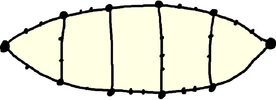
A simple ladder between and is a nonsingular disc diagram that is the union of a sequence of -cells such that each intersects and in a nontrivial boundary arc, and is a nontrivial internal arc when , and when , finally the startpoint of lies in the interior of , and the endpoint of lies in the interior of . See Figure 1.
Definition 3.3 (Quasigeodesic).
Let be a graph and let be the induced length metric when all edges have length 1. For real constants , a combinatorial path is a -quasigeodesic if for each subpath of between vertices and , the length is at most . A -quasigeodesic is called a -quasigeodesic.
Proposition 3.4 (Simple Ladder).
Let be a -hyperbolic graph. For each , there is an integer such that for all the following property holds:
If and are embedded -quasigeodesics with the same startpoint and endpoint, and with no common interior points. Then there is an embedded disc diagram between and such that is a simple ladder.
For the proof of Proposition 3.4, we recall the following well-known fact, a proof of which can found in [2, Chapter III.H, Corollary 1.8].
Lemma 3.5 (Slim rectangles).
Let be a -hyperbolic graph. For any there exists a constant with the following property. If is a closed path such that each is a -quasigeodesic, then each vertex of is contained in the -neighborhood of the set of vertices of .
Lemma 3.6 (Fellow traveling).
Let be a -hyperbolic graph. Let be an embedded -quasigeodesic, and let be a geodesic, such that have the same startpoint and endpoint. Let of Lemma 3.5. Suppose is the concatenation of edge-paths such that:
For each , let be a geodesic from the startpoint of to . Notice that and is an edge-path. For , let be the subpath of from the endpoint of to the endpoint of , and let be the subpath of from the endpoint of to the endpoint of .
Then and have at most one point in common when . Consequently, .
Proof.
First, is an edge-path for each since it starts and ends at 0-cells and is embedded. Moreover, for each by Lemma 3.5, since is a -quasigeodesic rectangle. Using this, and applying Lemma 3.5 again, the Hausdorff distance between and is at most , since is a -quasigeodesic rectangle.
Suppose that and have more than one point in common. It follows that the minimal distance between and is less than . Since is a geodesic, if then the minimal distance between and is at least . Therefore, we can assume that . Since is an embedded path, either is contained in or vice-versa. If then applying Lemma 3.5 twice, and using that each twice, we see that is contained in the neighborhood of . Since is a geodesic, this can only happen if .
The second conclusion follows from the first since the concatenation covering has no backtracks. ∎

Proof of Proposition 3.4.
Suppose that . Let be a geodesic between the common startpoints and endpoints of . We will describe the -skeleton of a disc diagram between and .
If , then is a circuit of length at most and thus bounds a disc diagram with a single -cell yielding the claim trivially.
We now assume that , and express as the concatenation with
As described in Lemma 3.6, the paths and are concatenations and with the following properties (See Figure 2):
- •
For each there is a geodesic (respectively ) from the startpoint of to the startpoint of (respectively, the startpoint of ) such that and (respectively ) have only one vertex in common.
- •
are edge-paths of length .
- •
Since and are geodesics with the same startpoint, by possibly re-choose them, we can assume that and where intersect only at their startpoint.
- •
The paths are disjoint if , and hence the same holds for .
Let denote the embedded path from the startpoint of to the startpoint of . It is immediate that . Since and are embedded with disjoint interior, the closed path is a circuit. Moreover, the circuits and intersect only if .
Notice that
The union of the circuits forms the -skeleton of an embedded simple ladder in between and . ∎
Theorem 3.7 below is a strong fellow traveling property property for hyperbolic fine graphs admitting a cocompact action. Its proof is an application of the definition of fine graph and Proposition 3.4.
Theorem 3.7 (Strong Fellow Travel Property).
Let be a fine hyperbolic graph, and let be a group acting on with finitely many orbits of edges.
Suppose the vertex set of is partitioned into subsets and such that no pair of vertices in are adjacent. Let be a proper metric on invariant under the action of .
For any , there exists a constant with the following property. If and are embedded -quasigeodesics between the same pair of vertices, then for any -vertex of there is a -vertex of such that .

Proof.
Let be sufficiently large so that satisfies the conclusion of Proposition 3.4 for the given . Since acts cocompactly on the fine graph , there is a finite number of boundary cycles of 2-cells in up to the action of . Combining this with is -equivariant shows that there is constant such that for any pair of -vertices in the boundary cycle of a 2-cell.
Let and be embedded -quasigeodesics in with the same startpoint and endpoint. Without loss of generality, assume that and have no common interior points.
By Proposition 3.4, there is an embedded simple ladder between and . Combining that each 2-cell of intersects both and in nontrivial arcs, and that no two -vertices are connected by an edge, it follows that each 2-cell of has -vertices in and in (See Figure 3). Since each -vertex of belongs to a 2-cell of , it follows that for any -vertex of there is a -vertex of such that . ∎
4. Equivalences of Formulations of Relative quasiconvexity
In this section we prove Theorem 1.7 on the equivalence between relative quasiconvexity of Definition 1.3, labelled by , and relative quasiconvexity of Definition 1.6, labelled by , in the context of countable relatively hyperbolic groups.
The argument introduces two auxiliary definitions of relative quasiconvexity, labelled by and , and then the theorem follows after proving the following equivalences:
| (1) |
The section is divided in six short parts as follows. First we recall the notion of coned-off Cayley graph, and deduce a strong version of the fellow travel property using the main result of Section 3. The second part shows that relative quasiconvexity of Definition 1.6, labelled by , implies finite relative generation. The third part state the two auxiliary definitions. The remaining three parts correspond to each of the three equivalences in illustration (1).
For the rest of the section, let be a hyperbolic group relative to a collection of subgroups , let be a finite relative generating set for , and let be a proper left-invariant metric on .
4.1. The Coned-off Cayley Graph
Definition 4.1 (Cayley Graph).
Let be a subset of a group , and assume that is closed under inverses. The Cayley graph is an oriented labelled 1-complex with vertex set and edge set . An edge goes from the vertex to the vertex and has label . Observe that is connected if and only if is a generating set of .
The notion of coned-off Cayley graph is originally due to Farb [4] and the following generalization is taking from [5, Sec. 3.4].
Definition 4.2 (Coned-off Cayley Graph ).
Let be a finite relative generating set for and assume that is closed under inverses. The coned-off Cayley graph is the graph constructed from the Cayley graph as follows: For each left coset with and , add a new vertex to , and add a -cell from this new vertex to each element of . These new vertices of that are not in are called cone-vertices. Each -cell of between an element of and a cone vertex is a cone-edge. Note that the coned-off Cayley graph is connected since is a relative generating set for .
There is a related (genuine) Cayley graph of with respect to the generating set defined as the disjoint union which we denote by .
Proposition 4.3 below appeared in Dahmani’s thesis [3, Proof Lemma A.4] and in Hruska’s work [5, Proof (RH-4) (RH-5)]. We included a proof using the results of Section 2.
Proposition 4.3.
Suppose that is a -graph. If is a finite relative generating set for , then there exists a -graph such that and both embed equivariantly and simplicially into .
In particular, is a -graph.

Proof.
We will perform finitely many arc -attachments to to obtain a graph where equivariantly embeds in . Then Lemmas 2.7 and 2.9 will imply that is a -graph, and that is a quasi-isometric embedding.
The graph is obtained as follows. By -attaching a triangle around an edge of , we obtain a new where acts freely on triangle-tops. See Figure 4. We identify with a triangle-top orbit. Performing an additional edge -attachment to for each element of yields a graph . Finally, for each group , choose a vertex stabilize by and perform a -attachment of an edge between and of to obtain a graph . Observe that equivariantly embeds in , and that is a -graph by Lemmas 2.7 and 2.9.
By Lemma 2.4, all infinite valence vertices of are contained in . Since has finitely many -orbits of edges, is obtained from after finitely many -removals of vertices of finite valence together with their adjacent vertices. Since is a -graph, Lemma 2.11 implies that is a -graph and that is a -equivariant quasi-isometry. ∎
Proposition 4.4 (Strong Fellow Travel for ).
Let be a finite relative generating set for , and let be a proper left-invariant metric on .
For any , there exists a constant with the following property. If and are embedded -quasigeodesics in between the same pair of elements of , then for each element of , there is an element of such that .
Proof.
Corollary 4.7 below is an analogous result to Proposition 4.4 for the Cayley graph . A version of this result for the case that is finitely generated appears as [9, Prop. 3.15]. Its hypothesis requires that the quasigeodesics do not backtrack in the following sense based on [9, Def. 3.9]:
Definition 4.5 (Phase Vertices and Backtracking in ).
Let be a path in . For a subgroup , a nontrivial subpath of is called a -component of if all edges of are labelled by elements of , in particular, all vertices of belong to the same left coset of .
An -component of is called maximal if it is not a proper subpath of -component of . The path is said to backtrack if has two disjoint and maximal -components for some . A vertex of is called a phase vertex if is not an interior vertex of a -component of .
Remark.
Since is a Cayley graph of with respect to the disjoint union , a -component and a -component of can not have edges in common if and are different.
Lemma 4.6 ( and are quasi-isometric).
The identity map of induces a natural -quasi-isometry with the following property. If is an embedded path, with only phase vertices, and without backtracking in , then is embedded in .
Proof.
The quasi-isometry maps edges labelled by elements of to the corresponding edge in , and edges labelled by an element of are map to a -path passing through a cone-vertex of a left coset of . Observe that if is embedded and is not embedded, then either contains a -component of length at least two, or backtracks. ∎
Corollary 4.7 (Strong Fellow Travel for ).
Let be a finite relative generating set for , and let be a proper left-invariant metric on .
For any , there exists a constant with the following property. If and are embedded -quasigeodesics without backtracking in between the same pair of elements of , then for each phase vertex of , there is a phase vertex of such that .
Proof.
Let be the quasi-isometry given by Lemma 4.6. If and contain only phase vertices, the conclusion follows immediately after mapping and to and applying Proposition 4.4.
The Corollary holds for general and after the following observation. Let be a -quasigeodesic in , and let be the path obtained from after replacing by a single edge each maximal -component (for each ). The new path contains only phase vertices, its vertex set equals the set of phase vertices of , and is also a -quasigeodesic (since the process from to is only shortening distances). ∎
4.2. Finite Relative Generation
Lemma 4.8 (Bounded Intersection).
Proof.
Suppose the statement is false for the constant . Then there are sequences and such that , , , and
Since balls are finite in the metric space , without loss of generality assume is a constant sequence . For any and , observe that , and hence and are in the same right coset of , say . It follows that
for any , a contradiction. ∎
Lemma 4.9 (Parabolic Approximation).
For each subgroup and each , there is with the following property: If is a product of the form where , , and for some . Then where , , and . (See Figure 5.)

Proof.
For each and , let be the constant provided by Lemma 4.8. Since is proper and is a finite collection of subgroups,
is a well-defined positive integer.
Suppose that is a product of the form where , , and for . Observe that
where the neighborhoods are in with respect to the metric , and the second inclusion is a consequence of Lemma 4.8. The conclusion of the lemma is immediate. ∎
Proposition 4.10 ( Finite Relative Generation).
Suppose that satisfies Definition 1.6 of relative quasiconvexity for a proper left-invariant metric on , and a constant . Then is finitely generated relative to the finite collection of subgroups
Proof.
Let , and let be the constant provided by Lemma 4.9. Let
We will show that is a finite relative generating set for with respect to the finite collection of subgroups .
Let , and let be a geodesic in from the identity element to . Here each is an (oriented) edge of . For each , there is an (oriented) path from the startpoint of to an element of such that the -distance between its endpoints is at most . Let be the element of defined as the difference between the endpoint and startpoint of , and the label of the (oriented) edge . Then let , and notice that and for each . See Figure 6.
If is labelled by an element of , that is , then
and hence .
Suppose that is labelled by a parabolic element, that is . Then the element can be approximated by a parabolic. Namely, by Lemma 4.9, where , , and . Hence is a product of an element of a subgroup in , and an element of .
It follows that each element can be expressed as a product of elements of and elements of the subgroups in . ∎

4.3. Auxiliary Definitions
Since acts on the connected graph with finitely many orbits of edges, an standard argument shows that is finitely generated relative to . This justifies the existence of finite relative generating sets in the following two definitions.
Definition 4.11 (() Auxiliary definition in ).
Let be a finite relative generating set for , and let be a proper left-invariant metric on . A subgroup of is quasiconvex relative to if there exists a constant such that the following holds: Let , be two elements of , and let be an arbitrary geodesic path from to in . For any non-cone vertex of , there exists a non-cone vertex in such that .
Definition 4.12 ( Second auxiliary definition in ).
Let be a finite relative generating set for . A subgroup of is quasiconvex relative to if there is a non-empty connected -invariant subgraph of that is quasi-isometrically embedded and has finitely many -orbits of edges.
4.4. The equivalence
Proposition 4.13 ().
Relative quasiconvexity of Definition 1.6 and relative quasiconvexity of Definition 4.11 are equivalent notions.
In particular, Definition 4.11 is independent of the generating set and the left-invariant metric on .
Proof.
Let be the natural quasi-isometry induced by the identity map on , see Lemma 4.6.
Suppose that satisfies Definition 4.11 for a constant . Let be a geodesic in between elements of . Then maps to a -quasigeodesic . Let be a geodesic in between the endpoints of . By Proposition 4.4, there is a constant such that for each non-cone vertex of , there is a non-cone vertex such that . By Definition 4.11, for each non-cone vertex of , there is such that . Since the vertices of map to the non-cone vertices of , it follows that for each vertex of , there is a vertex of such that . Therefore, satisfies Definition 1.6.
Conversely, suppose that satisfies Definition 1.6 for a constant , and let be a geodesic in between elements of . Let be a geodesic in between the endpoints of . Observe that there is an embedded -quasigeodesic in that maps onto by , has only phase vertices, and does not backtrack. Then Proposition 4.7 implies that there is a constant such that the vertices of and (and hence ) are -closed with respect to the metric . Since the vertices of are -close to the elements of with respect to , we conclude that satisfies Definition 4.11 for the constant . ∎
4.5. The equivalence
Proposition 4.14 ().
Proof.
Let be a proper left-invariant metric on , and let be a finite relative generating set of . Suppose that satisfies Definition 4.11 for some .
Choosing the subgraph . By Proposition 4.13, also satisfies relative quasiconvexity of Definition 1.6. Thus by Proposition 4.10, is generated by a finite subset relative to the finite collection of subgroups
where is positive constant. Without loss of generality assume that .
Let be the cone-vertices associated to the subgroups in . Let be a finite connected subgraph of containing . By Lemma 2.13 the graph is connected.
The inclusion is a quasi-isometric embedding with respect to the combinatorial path metrics. Let and denote the combinatorial path metrics of and respectively. Specifically we will show that there is a constant such that for any we have .
We define our constant with the help of four auxiliary constants. Let , and observe that since , is connected, and . Let , and notice that is a finite number since . Let be the constant provided by Lemma 4.9. Let
and notice that is finite since is a proper metric. Let .
Let and let be a geodesic in from to . Express as a concatenation of paths so that each is either a single edge with endpoints in , or is a shortcut consisting of two cone-edges meeting at a cone-point. Note that each shortcut has also endpoints in ). For each let denote the endpoint of .
Since satisfies Definition 4.11 for the constant , for each , there is an element with . Let denote the startpoint of and let denote the endpoint of .
If is a single edge, then , and therefore
If is a shortcut, then where , , and for some . By Lemma 4.9, where , , and . Since , the cone-vertex is contained in , and therefore Hence
To conclude, observe that
Proposition 4.15 ().
Proof.
Let be a proper left-invariant metric on , and let be a finite relative generating set of . Suppose that satisfies Definition 4.12.
Let be connected quasi-isometrically embedded subgraph of that is -equivariant and has finitely many -orbits of edges. The following statements about hold.
- (1)
Since is connected, it has at least one vertex that is not a cone-vertex. Without loss of generality, assume that the identity is a vertex of . In particular, we assume that all elements of are vertices of .
- (2)
Since acts cocompactly on , there is such that each vertex of is either a cone-vertex, or an element of is at distance at most from with respect to .
- (3)
Since is quasi-isometrically embedded subgraph of , there is such that any geodesic in is a -quasi-geodesic in .
Let be the constant provided by Proposition 4.4. Let be a geodesic in with endpoints in . Let be a geodesic in between the endpoints of . By Statement (3), is a -quasigeodesic. Therefore, Proposition 4.4 implies that for each non-cone vertex of , there is a non-cone vertex of such that . Combining this with Statement (2) shows that for each non-cone vertex of there is a non-cone vertex such that . Therefore, satisfies Definition 4.11. ∎
4.6. The equivalence
Proposition 4.16 ().
References
- [1] B.H. Bowditch. Relatively hyperbolic groups. preprint, 1999.
- [2] Martin R. Bridson and André Haefliger. Metric spaces of non-positive curvature, volume 319 of Grundlehren der Mathematischen Wissenschaften [Fundamental Principles of Mathematical Sciences]. Springer-Verlag, Berlin, 1999.
- [3] F. Dahmani. Les groupes relativement hyperboliques et leurs bords. PhD thesis, Univ. Louis Pasteur, Strasbourg, France, 2003.
- [4] B. Farb. Relatively hyperbolic groups. GAFA, Geom. funct. anal., 8(5):810–840, 1998.
- [5] G. Christopher Hruska. Relative hyperbolicity and relative quasiconvexity for countable groups. Algebr. Geom. Topol., 10(3):1807–1856, 2010.
- [6] Jason Fox Manning and Eduardo Martínez-Pedroza. Separation of relatively quasiconvex subgroups. Pacific J. Math., 244(2):309–334, 2010.
- [7] Eduardo Martínez-Pedroza. Combination of quasiconvex subgroups of relatively hyperbolic groups. Groups Geom. Dyn., 3(2):317–342, 2009.
- [8] Eduardo Martínez-Pedroza and Daniel T. Wise. Local quasiconvexity of groups acting on small cancellation complexes. J. Pure Appl. Algebra., to appear. Preprint at arXiv:1009.3407.
- [9] Denis V. Osin. Relatively hyperbolic groups: intrinsic geometry, algebraic properties, and algorithmic problems. Mem. Amer. Math. Soc., 179(843):vi+100, 2006.
- [10] Pekka Tukia. Conical limit points and uniform convergence groups. J. Reine Angew. Math., 501:71–98, 1998.