跳到论文正文
W Papers独立论文阅读器 arXiv:1009.3524 论文正文 计算阅读时间 · 0%
引用这篇论文根据当前论文元数据生成,正式投稿前建议核对。


License: arXiv.org perpetual non-exclusive license
arXiv:1009.3524v2 [math.DG] 20 Dec 2011

Minimal surfaces with limit ends in ℍ2×ℝ\mathbb{H}^{2}\times{\mathbb{R}}

M. Magdalena Rodríguez ††thanks: Research partially supported by a Spanish MEC-FEDER Grant no. MTM2007-61775, a Regional J. Andalucía Grant no. P09-FQM-5088 and "Grupo Singular" of the UCM.
Abstract

For any m⩾1m\geqslant 1, we construct properly embedded minimal surfaces in ℍ2×ℝ\mathbb{H}^{2}\times{\mathbb{R}} with genus zero, infinitely many vertical planar ends and mm limit ends. We also provide examples with an infinite countable number of limit ends. All these examples are vertical bi-graphs.

Mathematics Subject Classification: Primary 53A10, Secondary 49Q05, 53C42

1 Introduction

The theory of properly embedded minimal surfaces with genus zero (i.e. those which are topologically a punctured sphere) in Euclidean space ℝ3{\mathbb{R}}^{3} has been largely studied (see [1, 2, 8, 9] and the references therein). The final classification of such surfaces was given by Bill Meeks, Joaquín Pérez and Antonio Ros in [10]. The only examples with infinite topology are Riemann minimal surfaces. They form a 1-parameter family whose natural limits are the catenoid and the helicoid. When the planar ends are horizontally placed, each Riemann minimal example is invariant by a non-horizontal translation, its intersection with any horizontal plane is either a circle or a straight line, it has infinitely many annular ends asymptotic to horizontal planes, and has exactly two limit ends11 1 A limit end ee of a non-compact surface MM is an accumulation point of the set ℰ⁡(M)\mathcal{E}(M) of ends of MM. See [9].: one top and one bottom limit end.

Laurent Hauswirth [5] constructed Riemann-type minimal surfaces in ℍ2×ℝ\mathbb{H}^{2}\times{\mathbb{R}}, which are properly embedded and have genus zero, infinitely many ends asymptotic to horizontal slices and two limit ends: one top and one bottom limit end. It is natural to ask if there are examples of properly embedded minimal surfaces in ℍ2×ℝ\mathbb{H}^{2}\times{\mathbb{R}} with genus zero, infinitely many ends and m0m_{0} limit ends, with m0≠2m_{0}\neq 2. In this paper we construct examples for any m0≥1m_{0}\geq 1, and we also construct examples with an infinite countable number of limit ends.

In a joint work with Filippo Morabito [11], we have recently constructed a (2​k−3)(2k-3)-parameter family ℱk\mathcal{F}_{k} of properly embedded minimal surfaces in ℍ2×ℝ\mathbb{H}^{2}\times{\mathbb{R}} with total (intrinsic) curvature 4​π​(1−k)4\pi(1-k), genus zero and kk vertical planar ends (i.e. annular ends asymptotic to vertical geodesic planes), for any k⩾2k\geqslant 2. We call them minimal kk-noids. Each surface in this family is invariant by reflection symmetry about the horizontal slice ℍ2×{0}\mathbb{H}^{2}\times\{0\}. Pyo [13] has constructed independently a 1-parameter family of surfaces with the same properties. The examples given by Pyo, which are included in ℱk\mathcal{F}_{k}, are also invariant by reflection symmetry about kk vertical geodesic planes forming an angle π/k\pi/k. The examples with genus zero and infinitely many ends we construct in the present paper are obtained by taking limits when k→+∞k\to+\infty of certain surfaces Mk∈ℱkM_{k}\in\mathcal{F}_{k}.

The simple ends (i.e. non-limit ends) of the surfaces we construct are vertical planar ends. Fixed an orientation of ℍ2\mathbb{H}^{2}, we can order these simple ends cyclically. If a limit end can be obtained as accumulation of simple ends ordered following the negative orientation (resp. the positive orientation) but it cannot be obtained as accumulation of simple ends ordered following the positive orientation (resp. negative orientation), we will say that it is a left (resp. right) limit end. In other case, we will say that it is a 2-sided limit end.

Now we state the main results of this paper.

Theorem 1.1.

For any m0≥1m_{0}\geq 1, there exists a properly embedded minimal surface Σ\Sigma in ℍ2×ℝ\mathbb{H}^{2}\times{\mathbb{R}} with genus zero, infinitely many vertical planar ends and m0m_{0} limit ends, which is symmetric with respect to a horizontal slice (in fact, it is a vertical bi-graph). Moreover, if we denote by E∞1,…,E∞m0E_{\infty}^{1},\ldots,E_{\infty}^{m_{0}} the limit ends of Σ\Sigma, we can prescribe each E∞mE_{\infty}^{m} to be left, right or 2-sided.

If we take limits of appropriately chosen minimal surfaces in ℱk\mathcal{F}_{k}, we can also obtain properly embedded minimal surfaces in ℍ2×ℝ{\mathbb{H}^{2}}\times{\mathbb{R}} with genus zero, infinitely many vertical planar ends and an infinite countable number of limit ends.

Theorem 1.2.

There exists a properly embedded minimal surface in ℍ2×ℝ{\mathbb{H}^{2}}\times{\mathbb{R}} with genus zero, infinitely many vertical planar ends and an infinite countable number of limit ends {E∞m}m∈ℕ\{E_{\infty}^{m}\}_{m\in{\mathbb{N}}}, which is symmetric with respect to a horizontal slice (in fact, it is a vertical bi-graph). Moreover, we can prescribe each E∞mE_{\infty}^{m} to be left, right or 2-sided.

All the examples constructed in Theorems 1.1 and 1.2 are obtained by reflection symmetry about the horizontal slice ℍ2×{0}{\mathbb{H}^{2}}\times\{0\} from a vertical graph contained in ℍ2×[0,+∞){\mathbb{H}^{2}}\times[0,+\infty) whose boundary lies on ℍ2×{0}{\mathbb{H}^{2}}\times\{0\}.

The author would like to thank Joaquín Pérez for some helpful conversations.

2 Preliminaries

We consider the half-plane model of ℍ2{\mathbb{H}^{2}},

ℍ2={(x,y)∈ℝ2|y>0},\mathbb{H}^{2}=\{(x,y)\in{\mathbb{R}}^{2}\ |\ y>0\},

with the hyperbolic metric g−1=1y2​(d​x2+d​y2)g_{-1}=\frac{1}{y^{2}}(dx^{2}+dy^{2}). We denote by tt the coordinate in ℝ{\mathbb{R}} and consider in ℍ2×ℝ{\mathbb{H}^{2}}\times{\mathbb{R}} the usual product metric,

d​s2=1y2​(d​x2+d​y2)+d​t2.ds^{2}=\frac{1}{y^{2}}(dx^{2}+dy^{2})+dt^{2}.

Given an open domain Ω⊂ℍ2\Omega\subset{\mathbb{H}}^{2} and a smooth function u:Ω→ℝu:\Omega\to{\mathbb{R}}, the graph of uu is a minimal surface in ℍ2×ℝ{\mathbb{H}^{2}}\times{\mathbb{R}} when

(1) div⁡(∇u1+|∇u|2)=0,{\rm div}\left(\frac{\nabla u}{\sqrt{1+|\nabla u|^{2}}}\right)=0,

where all terms are calculated with respect to the metric of ℍ2{\mathbb{H}^{2}}.

Finally, we denote by ∂∞ℍ2\partial_{\infty}\mathbb{H}^{2} the infinite boundary of ℍ2\mathbb{H}^{2}, i.e.

∂∞ℍ2={(x,y)∈ℝ2|y=0}.\partial_{\infty}\mathbb{H}^{2}=\{(x,y)\in{\mathbb{R}}^{2}\ |\ y=0\}.

2.1 Flux of a minimal graph along a curve

Let uu be a minimal graph defined on a domain Ω⊂ℍ2\Omega\subset{\mathbb{H}^{2}}. Assume ∂Ω\partial\Omega is piecewise smooth and uu extends continuously to Ω¯\overline{\Omega} (possibly with infinite values). We define the flux of uu along a curve Γ⊂∂Ω\Gamma\subset\partial\Omega as

Fu​(Γ)=∫Γ⟨∇u1+|∇u|2,η⟩​𝑑s,F_{u}(\Gamma)=\int_{\Gamma}\left\langle\frac{\nabla u}{\sqrt{1+|\nabla u|^{2}}},\eta\right\rangle ds,

where η\eta is the outer normal to ∂Ω\partial\Omega in ℍ2{\mathbb{H}^{2}} and d​sds is the arc-length of ∂Ω\partial\Omega.

In the case Γ⊂Ω\Gamma\subset{\Omega}, we can see Γ\Gamma in the boundary of different subdomains of Ω{\Omega}, with two possible induced orientations. The flux Fu​(Γ)F_{u}(\Gamma) of uu along Γ{\Gamma} is then well-defined up to sign, and |Fu​(Γ)||F_{u}(\Gamma)| is well-defined.

Given an arc C⊂ℍ2C\subset{\mathbb{H}^{2}}, we will denote by |C||C| the length of CC in ℍ2{\mathbb{H}^{2}}. The proof of the following result can be found in [12], Lemmae 1 and 2.

Lemma 2.1 ([12]).

Let uu be a minimal graph on a domain Ω⊂ℍ2\Omega\subset{\mathbb{H}^{2}}.

  • (i)

    For every subdomain Ω′⊂Ω\Omega^{\prime}\subset\Omega such that Ω′¯\overline{{\Omega}^{\prime}} is compact, we have Fu​(∂Ω′)=0F_{u}(\partial\Omega^{\prime})=0.

  • (ii)

    Let CC be a piecewise smooth curve contained in the interior of Ω{\Omega}, or a convex curve in ∂Ω\partial\Omega where uu extends continuously and takes finite values. If CC has finite length, then |Fu​(C)|<|C||F_{u}(C)|<|C|.

  • (iii)

    Let T⊂∂ΩT\subset\partial\Omega be a geodesic arc of finite length such that uu diverges to +∞+\infty (resp. −∞-\infty) as one approaches TT within Ω\Omega. Then Fu​(T)=|T|F_{u}(T)=|T| (resp. Fu​(T)=−|T|F_{u}(T)=-|T|).

The last statement in Lemma 2.1 admits the following generalization.

Lemma 2.2 ([12]).

For each n∈ℕn\in{\mathbb{N}}, let unu_{n} be a minimal graph on a fixed domain Ω⊂ℍ2\Omega\subset{\mathbb{H}^{2}} which extends continuously to Ω¯\overline{\Omega}, and let TT be a geodesic arc of finite length in ∂Ω\partial\Omega.

  • (i)

    If {un}n\{u_{n}\}_{n} diverges uniformly to +∞+\infty on compact subsets of TT while remaining uniformly bounded in compact subsets of Ω\Omega, then Fun​(T)→|T|F_{u_{n}}(T)\to|T|.

  • (ii)

    If {un}n\{u_{n}\}_{n} diverges uniformly to +∞+\infty in compact subsets of Ω\Omega while remaining uniformly bounded on compact subsets of TT, then Fun​(T)→−|T|F_{u_{n}}(T)\to-|T|.

2.2 Divergence lines

Let Ω⊂ℍ2\Omega\subset{\mathbb{H}^{2}} be a polygonal domain (i.e. a domain whose edges are geodesic arcs of ℍ2{\mathbb{H}^{2}}) with vertices in ℍ2∪∂∞ℍ2\mathbb{H}^{2}\cup\partial_{\infty}\mathbb{H}^{2}, possibly infinitely many. Given a sequence {uk}k\{u_{k}\}_{k} of minimal graphs defined on Ω\Omega, we define its convergence domain as

ℬ={p∈Ω|{|∇uk(p)|}k is bounded},\mathcal{B}=\left\{p\in\Omega\ |\ \{|\nabla u_{k}(p)|\}_{k}\mbox{ is bounded}\right\},

and the divergence set of {uk}k\{u_{k}\}_{k} as

𝒟=Ω−ℬ.\mathcal{D}=\Omega-\mathcal{B}.

From Lemma 4.3 in [7], we know that the divergence set 𝒟\mathcal{D} is composed of geodesic arcs contained in Ω{\Omega}, called divergence lines, each one joining two points of ∂Ω\partial\Omega (including the vertices of Ω\Omega). The following proposition describes the convergence domain and the divergence set of a sequence of minimal graphs. Its proof can be found in [7], Lemmae 4.2 and 4.3 and Proposition 4.4.

Proposition 2.3 ([7]).

Let Ω⊂ℍ2\Omega\subset\mathbb{H}^{2} be a polygonal domain, and {uk}k\{u_{k}\}_{k} a sequence of minimal graphs on Ω\Omega. Suppose that 𝒟\mathcal{D} is a countable set of divergence lines. Then passing to a subsequence we have:

  1. 1.

    𝒟\mathcal{D} is composed of pairwise disjoint geodesic arcs contained in Ω{\Omega} (called divergence lines), each one joining two points in ∂Ω\partial\Omega (including the vertices of Ω\Omega).

  2. 2.

    {|Fuk​(T)|}k\{|F_{u_{k}}(T)|\}_{k} converges to |T||T| as k→+∞k\to+\infty, for any geodesic arc TT with finite length contained in a divergence line L⊂𝒟L\subset\mathcal{D}.

  3. 3.

    ℬ\mathcal{B} is an open set. Moreover, for any component Ω′\Omega^{\prime} of ℬ\mathcal{B} and any p∈Ω′p\in\Omega^{\prime}, {uk−uk​(p)}k\{u_{k}-u_{k}(p)\}_{k} converges uniformly on compact subsets of Ω′\Omega^{\prime} to a minimal graph u∞u_{\infty}.

2.3 Jenkins-Serrin graphs on semi-ideal polygonal domains

Let Ω\Omega be a polygonal domain. We say that Ω\Omega is semi-ideal when no two consecutive vertices of Ω{\Omega} are either in ℍ2\mathbb{H}^{2} or at ∂∞ℍ2\partial_{\infty}\mathbb{H}^{2} (see Figure 1). We call interior vertices of Ω{\Omega} to those which are contained in ℍ2{\mathbb{H}^{2}}; ideal vertices of Ω\Omega to those lying on ∂∞ℍ2\partial_{\infty}{\mathbb{H}^{2}}; and limit ideal vertices of Ω{\Omega} to the limit points of ideal vertices of Ω{\Omega}.

Refer to caption
Figure 1: Example of a convex Jenkins-Serrin semi-ideal polygonal domain which verifies condition (⋆)(\star).

Fix a semi-ideal polygonal domain Ω{\Omega} with a finite number of vertices p1,…,p2​kp_{1},\ldots,p_{2k} (cyclically ordered). We can assume the odd vertices p2​i−1p_{2i-1} are ideal, and then the even vertices p2​ip_{2i} are interior.

For each i=1,…,ki=1,\ldots,k, we call AiA_{i} (resp. BiB_{i}) the geodesic arc joining p2​i−1,p2​ip_{2i-1},p_{2i} (resp. p2​i,p2​i+1p_{2i},p_{2i+1}). We consider a horocycle H2​i−1H_{2i-1} at p2​i−1p_{2i-1}. Assume H2​i−1∩H2​j−1=∅H_{2i-1}\cap H_{2j-1}=\emptyset for any i≠ji\neq j. Given a polygonal domain 𝒫\mathcal{P} inscribed in Ω\Omega (i.e. a polygonal domain 𝒫⊂Ω\mathcal{P}\subset\Omega whose vertices are vertices of Ω\Omega, possibly at ∂∞ℍ2\partial_{\infty}{\mathbb{H}^{2}}), we denote by Γ⁡(𝒫)\Gamma(\mathcal{P}) the part of ∂𝒫\partial\mathcal{P} outside the horocycles (observe that Γ⁡(𝒫)=∂𝒫\Gamma(\mathcal{P})=\partial\mathcal{P} in the case all the vertices of 𝒫\mathcal{P} are interior). Also let us call

α⁡(𝒫)=∑i=1k|Ai∩Γ⁡(𝒫)|andβ⁡(𝒫)=∑i=1k|Bi∩Γ⁡(𝒫)|,{\alpha}(\mathcal{P})=\sum_{i=1}^{k}\left|A_{i}\cap\Gamma(\mathcal{P})\right|\qquad{\rm and}\qquad{\beta}(\mathcal{P})=\sum_{i=1}^{k}\left|B_{i}\cap\Gamma(\mathcal{P})\right|,

where we recall that |∙|=lengthℍ2(∙)|\bullet|=\mbox{length}_{\mathbb{H}^{2}}(\bullet). See Figure 1.

Definition 2.4.

Let Ω\Omega be a semi-ideal polygonal domain with a finite number of vertices p1,…,p2​kp_{1},\ldots,p_{2k}, where p2​i−1∈∂∞ℍ2p_{2i-1}\in\partial_{\infty}{\mathbb{H}^{2}} and p2​i∈ℍ2p_{2i}\in{\mathbb{H}^{2}}. We say that Ω\Omega is Jenkins-Serrin if for some choice of horocycles H2​i−1H_{2i-1} as above it holds:

  • (i)

    α⁡(Ω)=β⁡(Ω){\alpha}(\Omega)={\beta}(\Omega).

  • (ii)

    2​α​(𝒫)<|Γ⁡(𝒫)|2{\alpha}(\mathcal{P})<\left|\Gamma(\mathcal{P})\right| and 2​β​(𝒫)<|Γ⁡(𝒫)|2{\beta}(\mathcal{P})<\left|\Gamma(\mathcal{P})\right|, for every polygonal domain 𝒫\mathcal{P} inscribed in Ω\Omega, 𝒫≠Ω\mathcal{P}\neq\Omega.

We remark that condition (i) in the above definition does not depend on the choice of horocycles; and if the inequalities of condition (ii) are satisfied for some choice of horocycles, then they continue to hold for “smaller” horocycles (see the argument given by Pascal Collin and Harold Rosenberg in [3], pages 1884 and 1885). The following result is a particular case of Theorem 4.12 in [7].

Theorem 2.5 ([7]).

Let Ω\Omega be a semi-ideal polygonal domain with edges A1,B1,…,Ak,BkA_{1},B_{1},\ldots,A_{k},B_{k} (cyclically ordered). There exists a solution uu for the minimal graph equation (1) in Ω{\Omega} with boundary values

u|Ai=+∞andu|Bi=−∞,for any ​i=1,…,k,u|_{A_{i}}=+\infty\quad\mbox{and}\quad u|_{B_{i}}=-\infty,\quad\mbox{for any }\ i=1,\ldots,k,

if, and only if, Ω\Omega is a Jenkins-Serrin domain. Moreover, such a solution is unique up to an additive constant, when it exists.

Refer to caption
Figure 2: Example of a convex semi-ideal polygonal domain satisfying condition (⋆)(\star) which is not Jenkins-Serrin, since 2​α​(𝒫)>|Γ⁡(𝒫)|2{\alpha}(\mathcal{P})>|\Gamma(\mathcal{P})| because |A2∩Γ⁡(𝒫)|>|L∩Γ⁡(𝒫)||A_{2}\cap\Gamma(\mathcal{P})|>|L\cap\Gamma(\mathcal{P})|.

We will work with convex semi-ideal polygonal domains Ω{\Omega} satisfying the following additional condition (see Figures 1 and 2):

(⋆\star) There exists a choice of pairwise disjoint horocycles H2​i−1H_{2i-1} at the ideal
vertices p2​i−1∈∂∞ℍ2p_{2i-1}\in\partial_{\infty}{\mathbb{H}^{2}} such that
       distℍ2​(p2​i−2,H2​i−1)=distℍ2​(p2​i,H2​i−1)\mbox{dist}_{\mathbb{H}^{2}}(p_{2i-2},H_{2i-1})=\mbox{dist}_{\mathbb{H}^{2}}(p_{2i},H_{2i-1})
for any i=1,…,ki=1,\ldots,k, using the cyclical notation p0=p2​kp_{0}=p_{2k}.

We remark that condition (⋆\star) does not depend on the choice of horocycles H2​i−1H_{2i-1}, and it is equivalent to the existence of a horocycle C2​i−1C_{2i-1} at p2​i−1p_{2i-1} passing through p2​i−2,p2​ip_{2i-2},p_{2i}, for any i=1,…,ki=1,\ldots,k. We call D2​i−1D_{2i-1} the component of ℍ2−C2​i−1{\mathbb{H}^{2}}-C_{2i-1} whose only point of ∂∞ℍ2\partial_{\infty}{\mathbb{H}^{2}} at its infinite boundary is p2​i−1p_{2i-1} (i.e. D2​i−1D_{2i-1} is the horodisk at p2​i−1p_{2i-1} bounded by C2​i−1C_{2i-1}), and D2​i−1¯=D2​i−1∪C2​i−1\overline{D_{2i-1}}=D_{2i-1}\cup C_{2i-1}.

Before finishing this subsection, we describe geometrically when a semi-ideal polygonal domain with a finite number of vertices and satisfying condition (⋆\star) is a Jenkins-Serrin domain. See Figure 2.

Lemma 2.6.

Let Ω{\Omega} be a semi-ideal polygonal domain with vertices p1,…,p2​kp_{1},\ldots,p_{2k} cyclically ordered so that p2​i−1∈∂∞ℍ2p_{2i-1}\in\partial_{\infty}{\mathbb{H}}^{2} and p2​i∈ℍ2p_{2i}\in{\mathbb{H}^{2}}, for any i=1,…,ki=1,\ldots,k. Suppose Ω{\Omega} satisfies condition (⋆\star) above. Then the following assertions are equivalent:

  1. 1.

    Ω{\Omega} is a Jenkins-Serrin domain.

  2. 2.

    p2​j∈ℍ2−D2​i−1¯p_{2j}\in\mathbb{H}^{2}-\overline{D_{2i-1}}, for any jj and any i∉{j,j+1}i\not\in\{j,j+1\}.

Proof.

Before proving the lemma, let us fix some notation. For any i=1,…,ki=1,\ldots,k, consider the nested sequence of horocycles {H2​i−1​(n)}n\{H_{2i-1}(n)\}_{n} at p2​i−1p_{2i-1} contained in D2​i−1D_{2i-1} and converging to p2​i−1p_{2i-1} as n→+∞n\to+\infty, such that distℍ2​(H2​i−1​(n),C2​i−1)=n\mbox{dist}_{\mathbb{H}^{2}}\left(H_{2i-1}(n),C_{2i-1}\right)=n, for any nn. Then

distℍ2​(p2​i−2,H2​i−1​(n))=distℍ2​(p2​i,H2​i​(n))=n.\mbox{dist}_{\mathbb{H}^{2}}(p_{2i-2},H_{2i-1}(n))=\mbox{dist}_{\mathbb{H}^{2}}(p_{2i},H_{2i}(n))=n.

Let us now prove Lemma 2.6. First suppose Ω{\Omega} is Jenkins-Serrin and there exists some p2​j∈D2​i−1¯p_{2j}\in\overline{D_{2i-1}}, with i∉{j,j+1}i\not\in\{j,j+1\}. We then have

distℍ2​(p2​j,H2​i−1​(n))⩽n\mbox{dist}_{\mathbb{H}^{2}}(p_{2j},H_{2i-1}(n))\leqslant n

for nn large. Let LL be the geodesic arc from p2​jp_{2j} to p2​i−1p_{2i-1}, and 𝒫\mathcal{P} be the component of Ω−{\Omega}- containing AiA_{i} on its boundary (see Figure 2). Clearly, 𝒫\mathcal{P} is a polygonal domain inscribed in Ω{\Omega}. And, for this choice of horocycles H2​i−1​(n)H_{2i-1}(n), it holds |Aℓ∩Γ⁡(𝒫)|=n\left|A_{\ell}\cap\Gamma(\mathcal{P})\right|=n (resp. |Bℓ∩Γ⁡(𝒫)|=n\left|B_{\ell}\cap\Gamma(\mathcal{P})\right|=n) for any ℓ\ell such that Aℓ⊂∂𝒫A_{\ell}\subset\partial{\mathcal{P}} (resp. Bℓ⊂∂𝒫B_{\ell}\subset\partial{\mathcal{P}}). Thus β⁡(𝒫)=α⁡(𝒫)−n\beta(\mathcal{P})={\alpha}(\mathcal{P})-n, and then

|Γ⁡(𝒫)|=distℍ2​(p2​j,H2​i−1​(n))+α⁡(𝒫)+β⁡(𝒫)⩽2​α​(𝒫).|\Gamma(\mathcal{P})|=\mbox{dist}_{\mathbb{H}^{2}}(p_{2j},H_{2i-1}(n))+{\alpha}(\mathcal{P})+\beta(\mathcal{P})\leqslant 2{\alpha}(\mathcal{P}).

This holds for every nn large, which contradicts that Ω{\Omega} is a Jenkins-Serrin domain. This proves ​(1)⇒​(2)\emph{(1)}\Rightarrow\emph{(2)}.

Now assume p2​j∈ℍ2−D2​i−1¯p_{2j}\in\mathbb{H}^{2}-\overline{D_{2i-1}}, for any jj and any i∉{j,j+1}i\not\in\{j,j+1\}, and let us prove that Ω{\Omega} is a Jenkins-Serrin domain. As we have remarked above, we have α⁡(Ω)=β⁡(Ω){\alpha}({\Omega})={\beta}({\Omega}). Suppose there exists an inscribed polygonal domain 𝒫\mathcal{P} in Ω{\Omega}, 𝒫≠Ω\mathcal{P}\neq{\Omega}, such that

|Γ⁡(𝒫)|⩽2​α​(𝒫)|\Gamma(\mathcal{P})|\leqslant 2{\alpha}(\mathcal{P})

(the case |Γ⁡(𝒫)|⩽2​β​(𝒫)|\Gamma(\mathcal{P})|\leqslant 2{\beta}(\mathcal{P}) follows similarly). Since 𝒫≠Ω\mathcal{P}\neq{\Omega}, there is at least an interior geodesic γ1{\gamma}_{1} in ∂𝒫\partial{\mathcal{P}} (i.e. γ1⊂∂𝒫∩Ω{\gamma}_{1}\subset\partial{\mathcal{P}}\cap{\Omega}). We can assume there are no two consecutive interior geodesics γ1,γ2{\gamma}_{1},{\gamma}_{2} in ∂𝒫\partial{\mathcal{P}}: We would replace 𝒫\mathcal{P} by another inscribed polygonal domain satisfying the same properties as 𝒫\mathcal{P} by replacing γ1∪γ2{\gamma}_{1}\cup{\gamma}_{2} by the geodesic γ3{\gamma}_{3} such that γ1∪γ2∪γ3{\gamma}_{1}\cup{\gamma}_{2}\cup{\gamma}_{3} bounds a geodesic triangle contained in Ω{\Omega}. In a similar way, we can assume that

∂𝒫=Ai1∪γ1∪…∪Aij∪γj∪Aij+1∪…∪Ais∪γs,\partial{\mathcal{P}}=A_{i_{1}}\cup{\gamma}_{1}\cup\ldots\cup A_{i_{j}}\cup{\gamma}_{j}\cup A_{i_{j+1}}\cup\ldots\cup A_{i_{s}}\cup{\gamma}_{s},

where each γj{\gamma}_{j} is either an interior geodesic or a BiB_{i} edge, and at least γ1⊂Ω{\gamma}_{1}\subset{\Omega}. In particular, each γj{\gamma}_{j} joins an even vertex p2​ijp_{2i_{j}} to an odd vertex p2​ij+1−1p_{2i_{j+1}-1}. (Observe that, when γj{\gamma}_{j} is a BiB_{i} edge, then γj=Bij{\gamma}_{j}=B_{i_{j}} and ij+1=ij+1i_{j+1}=i_{j}+1.)

Hence ∑j=1s|γj∩Γ⁡(𝒫)|=|Γ⁡(𝒫)|−α⁡(𝒫)⩽α⁡(𝒫)=s​n\sum_{j=1}^{s}|{\gamma}_{j}\cap\Gamma(\mathcal{P})|=|\Gamma(\mathcal{P})|-{\alpha}(\mathcal{P})\leqslant{\alpha}(\mathcal{P})=sn, from where we deduce there must be an interior geodesic γj⊂∂𝒫{\gamma}_{j}\subset\partial{\mathcal{P}} whose length is smaller than or equal to nn. But this implies the vertex p2​ijp_{2i_{j}} lies on D¯2​ij+1−1\overline{D}_{2i_{j+1}-1} and ij∉{ij+1−1,ij+1}i_{j}\not\in\{i_{j+1}-1,i_{j+1}\}, a contradiction. ∎

2.4 Conjugate surfaces in ℍ2×ℝ{\mathbb{H}^{2}}\times{\mathbb{R}}

In this subsection we briefly recall how to obtain minimal surfaces in ℍ2×ℝ{\mathbb{H}^{2}}\times{\mathbb{R}} by conjugation from other known minimal examples. For more details see Daniel [4, Section 4] and Hauswirth, Sa Earp and Toubiana [6].

Let Σ\Sigma be a 2-sided minimal surface in ℍ2×ℝ{\mathbb{H}^{2}}\times{\mathbb{R}}. We call height function of Σ\Sigma to the horizontal projection h:Σ→ℝh:\Sigma\to{\mathbb{R}}, which is known to be a real harmonic map. And we denote by F:Σ→ℍ2F:\Sigma\to{\mathbb{H}^{2}} the vertical projection, which is a harmonic map, and by

Q=⟨Fz​F¯z⟩​(d​z)2Q=\langle F_{z}\bar{F}_{z}\rangle(dz)^{2}

the Hopf differential associated to FF, where zz is a local conformal coordinate on Σ\Sigma. Finally, we denote by NN a globally defined unit normal vector field on Σ\Sigma and by ν=⟨N,∂∂t⟩\nu=\langle N,\frac{\partial}{\partial t}\rangle the angle function of Σ\Sigma.

Theorem 2.7 ([4, 6]).

Let Σ\Sigma be a simply-connected minimal surface in ℍ2×ℝ{\mathbb{H}^{2}}\times{\mathbb{R}}. There exists a minimal surface Σ∗⊂ℍ2×ℝ\Sigma^{*}\subset{\mathbb{H}^{2}}\times{\mathbb{R}}, called conjugate surface of Σ\Sigma, such that:

  1. 1.

    Σ\Sigma and Σ∗\Sigma^{*} are isometric. (If we identify points in Σ\Sigma and Σ∗\Sigma^{*} via an isometry, we can assume that the angle function ν∗\nu^{*}, the height function h∗h^{*}, the vertical projection F∗F^{*} of Σ∗\Sigma^{*}, and the Hopf differential Q∗Q^{*} associated to F∗F^{*}, are all defined on Σ\Sigma.)

  2. 2.

    The angle functions ν,ν∗\nu,\nu^{*} coincide.

  3. 3.

    The height functions h,h∗h,h^{*} are real harmonic conjugate.

  4. 4.

    Q∗=−QQ^{*}=-Q.

The conjugate surface Σ∗\Sigma^{*} is well-defined up to an isometry of ℍ2×ℝ\mathbb{H}^{2}\times{\mathbb{R}}. Finally, the conjugation exchanges the following Schwarz reflections:

  • •

    The symmetry with respect to a vertical geodesic plane of ℍ2×ℝ\mathbb{H}^{2}\times{\mathbb{R}} containing a geodesic curvature line of Σ\Sigma becomes the rotation of ℍ2×ℝ\mathbb{H}^{2}\times{\mathbb{R}} by angle π\pi with respect to a horizontal geodesic contained in Σ∗\Sigma^{*}, and viceversa.

  • •

    The symmetry with respect to a horizontal slice containing a geodesic curvature line of Σ\Sigma becomes the rotation by angle π\pi with respect to a vertical straight line contained in Σ∗\Sigma^{*}, and viceversa.

We will use the above correspondence to study the conjugate surface of a minimal graph defined on a convex semi-ideal polygonal domain of ℍ2{\mathbb{H}^{2}}. The surface constructed in this way is a minimal graph (and consequently embedded), as ensured by the following Krust-type theorem.

Theorem 2.8 ([6]).

If Σ\Sigma is a minimal graph over a convex domain Ω{\Omega} of ℍ2{\mathbb{H}^{2}}, then Σ∗\Sigma^{*} is also a minimal graph over a (non-necessarily convex) domain Ω∗⊂ℍ2{\Omega}^{*}\subset{\mathbb{H}^{2}}.

2.5 Minimal kk-noids of ℍ2×ℝ{\mathbb{H}^{2}}\times{\mathbb{R}}

In this subsection we briefly explain the construction of the properly embedded minimal surfaces of ℍ2×ℝ\mathbb{H}^{2}\times{\mathbb{R}} given in [11, 13], which have genus zero, k≥2k\geq 2 vertical planar ends and finite total (intrinsic) curvature 4​π​(1−k)4\pi(1-k). We call them minimal kk-noids of ℍ2×ℝ{\mathbb{H}^{2}}\times{\mathbb{R}}.

Let Ω{\Omega} be a convex Jenkins-Serrin semi-ideal polygonal domain with 2​k2k vertices p1,…,p2​kp_{1},\ldots,p_{2k}, cyclically ordered, so that the even vertices p2​ip_{2i} are located in the interior of ℍ2{\mathbb{H}^{2}}, and the odd vertices p2​i−1p_{2i-1} are at ∂∞ℍ2\partial_{\infty}{\mathbb{H}}^{2}, for i=1,…,ki=1,\ldots,k. We call AiA_{i} the edge of Ω{\Omega} whose endpoints are p2​i−1,p2​ip_{2i-1},p_{2i}, and BiB_{i} the edge of Ω{\Omega} whose endpoints are p2​i,p2​i+1p_{2i},p_{2i+1}. We also require that Ω{\Omega} satisfies the condition (⋆\star) defined in Subsection 2.3.

By Theorem 2.5, there exists a unique solution uu to the minimal graph equation (1) defined over Ω{\Omega} with boundary values +∞+\infty on AiA_{i} and −∞-\infty on BiB_{i} such that u⁡(p0)=0u(p_{0})=0, for some fixed point p0∈Ωp_{0}\in\Omega. Denote by Σ\Sigma the graph surface of uu; Σ\Sigma is bounded by the kk vertical straight lines Γi={p2​i}×ℝ\Gamma_{i}=\{p_{2i}\}\times{\mathbb{R}}, i=1,…,ki=1,\ldots,k.

Refer to caption
Figure 3: Vertical projection of the conjugate surface Σ∗\Sigma^{*} in a symmetric case.

The conjugate surface Σ∗\Sigma^{*} of Σ\Sigma is a minimal graph over a (non-necessarily convex) domain Ω∗⊂ℍ2{\Omega}^{*}\subset{\mathbb{H}^{2}}, by Theorem 2.8 (see Figure 3). And ∂Σ∗\partial\Sigma^{*} consists of kk horizontal geodesic curvature lines Γi∗\Gamma_{i}^{*}. In [11] it is proved that Γi∗⊂ℍ2×{0}\Gamma_{i}^{*}\subset{\mathbb{H}^{2}}\times\{0\} for any ii and that Σ∗\Sigma^{*} is contained in one of the half-spaces determined by ℍ2×{0}{\mathbb{H}^{2}}\times\{0\}. By reflecting Σ∗\Sigma^{*} with respect to ℍ2×{0}{\mathbb{H}^{2}}\times\{0\}, we get a properly embedded minimal surface MM with genus zero and kk vertical planar ends, which has total (intrinsic) curvature 4​π​(1−k)4\pi(1-k). The ends of MM are asymptotic to the vertical geodesic planes ηi∗×ℝ\eta_{i}^{*}\times{\mathbb{R}}, where the ηi∗\eta_{i}^{*} are the complete geodesics such that ∂Ω∗=Γ1∗∪η1∗∪…∪Γk∗∪ηk∗\partial{\Omega}^{*}={\Gamma}_{1}^{*}\cup\eta_{1}^{*}\cup\ldots\cup{\Gamma}_{k}^{*}\cup\eta_{k}^{*} (cyclically ordered).

3 Proof of Theorem 1.1: examples with m0m_{0} limit ends

Firstly, let us recall some definitions. A limit end ee of a non-compact surface MM is an accumulation point of the set ℰ⁡(M)\mathcal{E}(M) of ends of MM. This makes sense since ℰ⁡(M)\mathcal{E}(M) can be endowed with a natural topology for which it is a compact, totally disconnected subspace of the real interval [0,1][0,1]. See [9] for more details. We call simple ends of MM to its non-limit ends.

Assume the simple ends of MM are asymptotic to vertical geodesic planes (called vertical planar ends) which can be ordered cyclically22 2 The surface MM we want to construct will be obtained as a limit of minimal kk-noids, and it is got by reflection symmetry from a minimal graph with boundary values 0,+∞0,+\infty, alternately. The vertical projection of MM will be bounded by strictly concave curves Γi∗\Gamma_{i}^{*} and geodesic curves ηi∗\eta_{i}^{*}, disposed alternately and asymptotic at ∂∞ℍ2\partial_{\infty}{\mathbb{H}^{2}}. The ends of MM will be asymptotic to the vertical geodesic planes ηi∗×ℝ\eta_{i}^{*}\times{\mathbb{R}}, which are cyclically ordered., fixed an orientation of ∂∞ℍ2\partial_{\infty}{\mathbb{H}^{2}}. If the limit end can be obtained as accumulation of simple ends ordered following the negative orientation (resp. the positive orientation) but it cannot be obtained as accumulation of simple ends ordered following the positive orientation (resp. negative orientation), we will say that it is a left (resp. right) limit end. In other case, we will say that it is a 2-sided limit end.

In this section we construct properly embedded minimal surfaces in ℍ2×ℝ{\mathbb{H}^{2}}\times{\mathbb{R}} with genus zero, infinitely many vertical planar ends and m0m_{0} limit ends, for any m0≥1m_{0}\geq 1. Furthermore, we can prescribe the behavior of the limit ends; more precisely, if we denote by E∞1,…,E∞m0E_{\infty}^{1},\ldots,E_{\infty}^{m_{0}} (cyclically ordered) the limit ends of such a surface, we can prescribe if each E∞mE_{\infty}^{m} is either a left, a right or a 2-sided limit end.

Now let us explain our construction. In a first step we will construct, by taking limits of convex Jenkins-Serrin semi-ideal polygonal domains Ωk{\Omega}_{k} with finitely many vertices, a convex semi-ideal polygonal domain Ω∞{\Omega}_{\infty} with an infinite countable set 𝒮\mathcal{S} of ideal vertices and m0{m_{0}} limit points p∞1,…,p∞m0p_{\infty}^{1},\ldots,p_{\infty}^{m_{0}} (cyclically ordered) such that, if E∞mE_{\infty}^{m} is prescribed to be a left (resp. a right or a 2-sided) limit end, then p∞mp_{\infty}^{m} is a left (resp. a right or a 2-sided) limit point, see Definition 3.1 below. We will say that such a limit point p∞mp_{\infty}^{m} is a left (resp. a right or a 2-sided) limit ideal vertex of Ω∞{\Omega}_{\infty}.

Definition 3.1.

Let 𝒮\mathcal{S} be a set of points in ∂∞ℍ2={y=0}\partial_{\infty}{\mathbb{H}^{2}}=\{y=0\}. We will say that p∞∈𝒮p_{\infty}\in\mathcal{S} is a limit point if every neighborhood of p∞p_{\infty} in ∂∞ℍ2\partial_{\infty}{\mathbb{H}^{2}} contains a point of 𝒮\mathcal{S} other than p∞p_{\infty} itself; i.e. if p∞=(x∞,0)p_{\infty}=(x_{\infty},0), then 𝒮∩{y=0, 0<|x−x∞|<ε}≠∅\mathcal{S}\cap\{y=0,\ 0<|x-x_{\infty}|<{\varepsilon}\}\neq\emptyset for every ε>0{\varepsilon}>0; or p∞=∞p_{\infty}=\infty and 𝒮∩{y=0,|x|>M}≠∅\mathcal{S}\cap\{y=0,\ |x|>M\}\neq\emptyset for every M>0M>0.

A limit point p∞=(x∞,0)p_{\infty}=(x_{\infty},0) of 𝒮\mathcal{S} is said to be a left (resp. a right) limit point if there exists some ε>0{\varepsilon}>0 such that 𝒮∩{−ε<x−x∞<0}=∅\mathcal{S}\cap\{-{\varepsilon}<x-x_{\infty}<0\}=\emptyset (resp. 𝒮∩{0<x−x∞<ε}=∅\mathcal{S}\cap\{0<x-x_{\infty}<{\varepsilon}\}=\emptyset); and it is said to be a 2-sided limit point in other case.

If p∞=∞p_{\infty}=\infty is a limit point of 𝒮\mathcal{S}, we say that it is a left (resp. a right) limit point if there exists some M>0M>0 such that 𝒮∩{x>M}=∅\mathcal{S}\cap\{x>M\}=\emptyset (resp. 𝒮∩{x<−M}=∅\mathcal{S}\cap\{x<-M\}=\emptyset); and it is a 2-sided limit point in other case.

Next we will get a Jenkins-Serrin minimal graph Σ\Sigma over Ω∞{\Omega}_{\infty} as a limit of Jenkins-Serrin minimal graphs over the Ωk{\Omega}_{k} domains. Finally, we will prove that the conjugate surface of Σ\Sigma is a minimal graph Σ∗⊂ℍ2×[0,+∞)\Sigma^{*}\subset{\mathbb{H}^{2}}\times[0,+\infty) whose boundary, which consists of horizontal geodesic curvature lines, is contained in the horizontal slice ℍ2×{0}{\mathbb{H}^{2}}\times\{0\}. The desired surface is obtained from Σ∗\Sigma^{*} by reflection symmetry about ℍ2×{0}{\mathbb{H}^{2}}\times\{0\}.

3.1 Construction of the domains

This subsection deals with the construction of the convex semi-ideal polygonal domain Ω∞{\Omega}_{\infty} in the argument explained above. We will construct a sequence of convex Jenkins-Serrin semi-ideal polygonal domains Ωk{\Omega}_{k} satisfying condition (⋆)(\star) defined in Subsection 2.3, each Ωk{\Omega}_{k} with a finite number of vertices, with Ωk⊂Ωk+1{\Omega}_{k}\subset{\Omega}_{k+1} for any kk, and such that they converge to a domain Ω∞{\Omega}_{\infty} in the desired conditions.

Consider m0m_{0} different ideal points in ∂∞ℍ2\partial_{\infty}{\mathbb{H}^{2}}:

p∞1=∞,p∞2=(x∞2,0),…,p∞m0=(x∞m0,0),p^{1}_{\infty}=\infty,\ p^{2}_{\infty}=(x_{\infty}^{2},0),\ldots,\ p^{m_{0}}_{\infty}=(x_{\infty}^{m_{0}},0),

with −∞<x∞2<…<x∞m0<+∞-\infty<x_{\infty}^{2}<\ldots<x_{\infty}^{m_{0}}<+\infty, when m0≥2m_{0}\geq 2; in the case m0=1m_{0}=1, we only have p∞1=∞p_{\infty}^{1}=\infty. These points will be the limit ideal vertices of Ω∞{\Omega}_{\infty}.

We call ℳ={m∈ℕ| 1≤m≤m0}\mathcal{M}=\{m\in{\mathbb{N}}\ |\ 1\leq m\leq m_{0}\}. For any m∈ℳm\in\mathcal{M}, choose two ideal points p−1m=(x−1m,0),p1m=(x1m,0)p_{-1}^{m}=(x_{-1}^{m},0),\ p_{1}^{m}=(x_{1}^{m},0) with x∞m<x−1m<x1m<x∞m+1x_{\infty}^{m}<x_{-1}^{m}<x_{1}^{m}<x_{\infty}^{m+1}, where x∞1=−∞x_{\infty}^{1}=-\infty and x∞m0+1=+∞x_{\infty}^{m_{0}+1}=+\infty.

Refer to caption
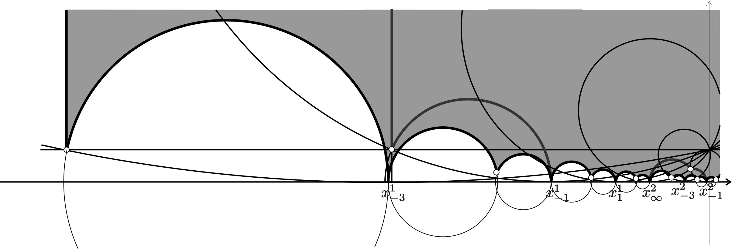
Figure 4: The shadowed region is an example of Ω1{\Omega}_{1} for three limit ideal vertices, where p∞1=∞{p^{1}_{\infty}=\infty} and pim=(xim,0)p^{m}_{i}=(x^{m}_{i},0) for the remaining values of i,mi,m. The interior vertices in white correspond, from the left to the right, to q−21,p01,q21,q−22,p02,q22,q−23,p03,q23q_{-2}^{1},p_{0}^{1},q_{2}^{1},q_{-2}^{2},p_{0}^{2},q_{2}^{2},q_{-2}^{3},p_{0}^{3},q_{2}^{3}.

For any m∈ℳm\in\mathcal{M} and any j∈{−1,1,∞}j\in\{-1,1,\infty\}, we call CjmC^{m}_{j} the horocycle at pjmp^{m}_{j} passing through P0=(0,1)P_{0}=(0,1). Denote by p0mp_{0}^{m} (resp. q−2m,q2mq_{-2}^{m},\ q_{2}^{m}) the point in C−1m∩C1mC_{-1}^{m}\cap C_{1}^{m} (resp. C∞m∩C−1mC_{\infty}^{m}\cap C_{-1}^{m}, C1m∩C∞m+1C_{1}^{m}\cap C_{\infty}^{m+1}) which is different from P0P_{0}, see Figure 4. We define Ω1{\Omega}_{1} as the semi-ideal polygonal domain with set of vertices

{p∞m,q−2m,p−1m,p0m,p1m,q2m|m∈ℳ}.\{p_{\infty}^{m},q_{-2}^{m},p_{-1}^{m},p_{0}^{m},p_{1}^{m},q_{2}^{m}\ |\ m\in\mathcal{M}\}.

By definition of q−2m,p0m,q2mq_{-2}^{m},p_{0}^{m},q_{2}^{m}, it is clear that Ω1{\Omega}_{1} satisfies condition (⋆)(\star). Now let us see we can choose the ideal vertices p−1m,p1mp_{-1}^{m},p_{1}^{m} to assure Ω1{\Omega}_{1} is convex. It suffices to choose appropriately x−1m,x1mx_{-1}^{m},x_{1}^{m} such that q−2m,p0m,q2m⊂{0<y<1}q_{-2}^{m},p_{0}^{m},q_{2}^{m}\subset\{0<y<1\}, except for q−21,q2m0∈{y=1}q_{-2}^{1},q_{2}^{m_{0}}\in\{y=1\}.

  • •

    If x∞m≥0x_{\infty}^{m}\geq 0 or x∞m+1≤0x_{\infty}^{m+1}\leq 0, then x−1m,x1mx_{-1}^{m},x_{1}^{m} can be chosen arbitrarily.

  • •

    In the case x∞m<0<x∞m+1x_{\infty}^{m}<0<x_{\infty}^{m+1}, we take max⁡{x∞m,−1}<x−1m<0<x1m<min⁡{x∞m+1,1}\max\{x_{\infty}^{m},-1\}<x_{-1}^{m}<0<x_{1}^{m}<\min\{x_{\infty}^{m+1},1\}.

With the choice above, the domain Ω1{\Omega}_{1} is convex. Finally, let us check that Ω1{\Omega}_{1} is a Jenkins-Serrin domain. Using Lemma 2.6 it suffices to get that p0mp_{0}^{m} (resp. q−2mq_{-2}^{m}; q2mq_{2}^{m}) lies outside Cjm′C_{j}^{m^{\prime}}, for any j∈{−1,1,∞}j\in\{-1,1,\infty\} and any m′∈ℳm^{\prime}\in\mathcal{M} such that Cjm′C_{j}^{m^{\prime}} is different from C−1mC_{-1}^{m}, C1mC_{1}^{m} (resp. C∞mC_{\infty}^{m}, C−1mC_{-1}^{m}; C1mC_{1}^{m}, C∞m+1C_{\infty}^{m+1}). By the choice above, this is the case when Cjm′=C∞1C_{j}^{m^{\prime}}=C_{\infty}^{1}. Let us assume Cjm′≠C∞1C_{j}^{m^{\prime}}\neq C_{\infty}^{1}. We prove it for p0mp_{0}^{m} (for q−2mq_{-2}^{m} q2mq_{2}^{m} it can be obtained similarly): If we denote p0m=(x0m,y0m)p_{0}^{m}=(x_{0}^{m},y_{0}^{m}), we have x−1m<x0m<x1mx_{-1}^{m}<x_{0}^{m}<x_{1}^{m}. If xjm′>x1mx_{j}^{m^{\prime}}>x_{1}^{m} (resp. xjm′<x−1mx_{j}^{m^{\prime}}<x_{-1}^{m}), then Cjm′C_{j}^{m^{\prime}} divides C1mC_{1}^{m} (resp. C−1mC_{-1}^{m}) in two components, one of them containing both p0mp_{0}^{m} and p1mp_{1}^{m} (resp. p−1mp_{-1}^{m}). That says that p0mp_{0}^{m} is outside Cjm′C_{j}^{m^{\prime}}.

Now we consider the subsets of ℳ\mathcal{M} given by

ℳ+={m∈ℳ|E∞m+1 is prescribed to be either a right or a 2-sided limit end},\mathcal{M}^{+}=\{m\in\mathcal{M}\ |\ E_{\infty}^{m+1}\ \mbox{ is prescribed to be either a right or a 2-sided limit end}\},
ℳ−={m∈ℳ|E∞m is prescribed to be either a left or a 2-sided limit end}.\mathcal{M}^{-}=\{m\in\mathcal{M}\ |\ E_{\infty}^{m}\ \mbox{ is prescribed to be either a left or a 2-sided limit end}\}.

For any k≥2k\geq 2, we define Ωk{\Omega}_{k} as the semi-ideal polygonal domain with set of vertices 𝒱k−∪𝒱0∪𝒱k+\mathcal{V}_{k}^{-}\cup\mathcal{V}^{0}\cup\mathcal{V}_{k}^{+}, where

𝒱k−={q−2​km,p1−2​km,p2−2​km,…,p−3m,p−2m|m∈ℳ−}∪{q−2m|m∈ℳ−ℳ−},\mathcal{V}_{k}^{-}=\{q_{-2k}^{m},p_{1-2k}^{m},p_{2-2k}^{m},\ldots,p_{-3}^{m},p_{-2}^{m}\ |\ m\in\mathcal{M}^{-}\}\cup\{q_{-2}^{m}\ |\ m\in\mathcal{M}-\mathcal{M}^{-}\},
𝒱k0={p∞m,p−1m,p0m,p1m|m∈ℳ},\mathcal{V}_{k}^{0}=\{p_{\infty}^{m},p_{-1}^{m},p_{0}^{m},p_{1}^{m}\ |\ m\in\mathcal{M}\},
𝒱k+={p2m,p3m,…,p2​k−2m,p2​k−1m,q2​km|m∈ℳ+}∪{q2m|m∈ℳ−ℳ+}.\mathcal{V}_{k}^{+}=\{p_{2}^{m},p_{3}^{m},\ldots,p_{2k-2}^{m},p_{2k-1}^{m},q_{2k}^{m}\ |\ m\in\mathcal{M}^{+}\}\cup\{q_{2}^{m}\ |\ m\in\mathcal{M}-\mathcal{M}^{+}\}.

and the vertices p±im,q±2​kmp_{\pm i}^{m},q_{\pm 2k}^{m} are defined by induction as follows:

  1. 1.

    Suppose that m∈ℳ+m\in\mathcal{M}^{+} and that we have defined the ideal vertices

    p1m=(x1m,0),…,p2​k−1m=(x2​k−1m,0),p_{1}^{m}=(x_{1}^{m},0),\ \ldots,\ p_{2k-1}^{m}=(x_{2k-1}^{m},0),

    with k≥1k\geq 1 and x1m<…<x2​k−1m<x∞mx_{1}^{m}<\ldots<x_{2k-1}^{m}<x_{\infty}^{m}. These ideal vertices determine the following data: For 1≤i≤k1\leq i\leq k,

    • •

      let C2​i−1mC_{2i-1}^{m} be the horocycle at p2​i−1mp_{2i-1}^{m} passing through P0P_{0};

    • •

      p2​i−2mp_{2i-2}^{m} is defined as the intersection point in C2​i−3m∩C2​i−1mC_{2i-3}^{m}\cap C_{2i-1}^{m} different from P0P_{0};

    • •

      q2​imq_{2i}^{m} is the intersection point in C2​i−1m∩C∞m+1C_{2i-1}^{m}\cap C_{\infty}^{m+1} different from P0P_{0}.

    This choice of p2​i−2m,q2​imp_{2i-2}^{m},q_{2i}^{m} will assure that Ωk{\Omega}_{k} is a convex Jenkins-Serrin semi-ideal polygonal domain which satisfies condition (⋆)(\star).

    Let us now define p2​k+1mp_{2k+1}^{m}. We call Γ2​km\Gamma_{2k}^{m} (resp. γ2​km\gamma_{2k}^{m}) the complete geodesic curve with endpoint p2​k−1mp_{2k-1}^{m} (resp. p∞m+1p^{m+1}_{\infty}) passing through q2​kmq_{2k}^{m}. Let (a2​km,0)(a_{2k}^{m},0) (resp. (b2​km,0)(b_{2k}^{m},0)) be the endpoint of Γ2​km\Gamma_{2k}^{m} (resp. γ2​km\gamma_{2k}^{m}) different from p2​k−1mp_{2k-1}^{m} (resp. p∞m+1p^{m+1}_{\infty}). We take p2​k+1m=(x2​k+1m,0)p_{2k+1}^{m}=(x_{2k+1}^{m},0) satisfying b2​km≤x2​k+1m≤a2​kmb_{2k}^{m}\leq x_{2k+1}^{m}\leq a_{2k}^{m}. We consider that property for p2​k+1mp_{2k+1}^{m} in order to get Ωk⊂Ωk+1{\Omega}_{k}\subset{\Omega}_{k+1}.

    We remark that both p2​k+1mp_{2k+1}^{m} and p2​kmp^{m}_{2k} converge to p∞m+1p_{\infty}^{m+1} as k→+∞k\to+\infty.

    Refer to caption
    Figure 5: The shadowed region is a piece of Ω2{\Omega}_{2}, with 1∈ℳ−−ℳ+1\in\mathcal{M}^{-}-\mathcal{M}^{+} and 2∈ℳ−2\in\mathcal{M}^{-}.
  2. 2.

    The corresponding definition for m∈ℳ−m\in\mathcal{M}^{-} follows analogously: Suppose m∈ℳ−m\in\mathcal{M}^{-} and that, for k≥1k\geq 1, we have defined the ideal vertices

    p1−2​km=(x1−2​km,0),…,p−1m=(x−1m,0),p_{1-2k}^{m}=(x_{1-2k}^{m},0),\ \ldots,\ p_{-1}^{m}=(x_{-1}^{m},0),

    with x∞m<x1−2​km<…<x−1mx_{\infty}^{m}<x_{1-2k}^{m}<\ldots<x_{-1}^{m}. These ideal vertices determine the following data: For 1≤i≤k1\leq i\leq k,

    • •

      let C1−2​imC_{1-2i}^{m} be the horocycle at p1−2​imp_{1-2i}^{m} passing through P0P_{0};

    • •

      p2−2​imp_{2-2i}^{m} is defined as the intersection point in C1−2​im∩C3−2​imC_{1-2i}^{m}\cap C_{3-2i}^{m} different from P0P_{0};

    • •

      q−2​imq_{-2i}^{m} is the intersection point in C∞m∩C1−2​imC_{\infty}^{m}\cap C_{1-2i}^{m} different from P0P_{0}.

    Let us now define p−1−2​kmp_{-1-2k}^{m}. We call Γ−2​km\Gamma_{-2k}^{m} (resp. γ−2​km\gamma_{-2k}^{m}) the complete geodesic curve with endpoint p1−2​kmp_{1-2k}^{m} (resp. p∞mp^{m}_{\infty}) passing through q−2​kmq_{-2k}^{m}. Let (a−2​km,0)(a_{-2k}^{m},0) (resp. (b−2​km,0)(b_{-2k}^{m},0)) be the endpoint of Γ−2​km\Gamma_{-2k}^{m} (resp. γ−2​km\gamma_{-2k}^{m}) different from p1−2​kmp_{1-2k}^{m} (resp. p∞mp^{m}_{\infty}). We choose p−1−2​km=(x−1−2​km,0)p_{-1-2k}^{m}=(x_{-1-2k}^{m},0), with b−2​km≤x−1−2​km≤a−2​kmb_{-2k}^{m}\leq x_{-1-2k}^{m}\leq a_{-2k}^{m}. With this choice of ideal vertices, we get Ωk⊂Ωk+1\Omega_{k}\subset\Omega_{k+1} and that both p−1−2​kmp_{-1-2k}^{m} and p−2​kp_{-2k} converges to p∞mp_{\infty}^{m} as k→+∞k\to+\infty.

By definition of the interior vertices p2​i−2m,q2​imp_{2i-2}^{m},q_{2i}^{m}, the semi-ideal polygonal domain Ωk{\Omega}_{k} satisfies condition (⋆)(\star). As x2​k−1mx_{2k-1}^{m} has the same sign as x2​k−3mx_{2k-3}^{m} and x∞m+1x_{\infty}^{m+1}, then p2​i−2m,q2​im⊂{0<y<1}p_{2i-2}^{m},q_{2i}^{m}\subset\{0<y<1\}. That fact assures that Ωk{\Omega}_{k} is convex. Moreover, as the horocycles Cjm′C_{j}^{m^{\prime}} can be ordered from the left to the right and they all pass through P0P_{0}, we can deduce (as in the case of Ω1{\Omega}_{1}) that the interior vertices p2​imp_{2i}^{m}, q−2​kmq_{-2k}^{m}, q2​kmq_{2k}^{m} are outside the horocycles Cjm′C_{j}^{m^{\prime}}, except for those used for defining them (i.e. their consecutive ones). Then Ωk{\Omega}_{k} is a Jenkins-Serrin domain, by Lemma 2.6.

Finally, we have defined the ideal vertices p2​i−1mp_{2i-1}^{m} to get Ωk⊂Ωk+1{\Omega}_{k}\subset{\Omega}_{k+1}; for instance, when m∈ℳ+m\in\mathcal{M}^{+} and kk is positive, the geodesics Akm,Bkm,A~k+1mA^{m}_{k},B^{m}_{k},\widetilde{A}^{m}_{k+1} do not intersect A~km\widetilde{A}^{m}_{k}, where AkmA^{m}_{k} (resp. Bkm;A~k+1m;A~kmB^{m}_{k};\widetilde{A}^{m}_{k+1};\widetilde{A}^{m}_{k}) is defined as the geodesic arc joining p2​k−1m,p2​kmp^{m}_{2k-1},p^{m}_{2k} (resp. p2​km,p2​k+1mp^{m}_{2k},p^{m}_{2k+1}; p2​k+1m,q2​k+2mp^{m}_{2k+1},q^{m}_{2k+2}; p2​k−1m,q2​kmp^{m}_{2k-1},q^{m}_{2k}).

Let Ω∞{\Omega}_{\infty} be the semi-ideal polygonal domain with set of vertices 𝒱∞−∪𝒱0∪𝒱∞+\mathcal{V}_{\infty}^{-}\cup\mathcal{V}^{0}\cup\mathcal{V}_{\infty}^{+}, where

𝒱∞−={p−2​km,p1−2​km|m∈ℳ−,k∈ℕ}∪{q−2m|m∈ℳ−ℳ−},\mathcal{V}_{\infty}^{-}=\{p_{-2k}^{m},p_{1-2k}^{m}\ |\ m\in\mathcal{M}^{-},\ k\in{\mathbb{N}}\}\cup\{q_{-2}^{m}\ |\ m\in\mathcal{M}-\mathcal{M}^{-}\},
𝒱∞+={p2​k−1m,p2​km|m∈ℳ+,k∈ℕ}∪{q2m|m∈ℳ−ℳ+}.\mathcal{V}_{\infty}^{+}=\{p_{2k-1}^{m},p_{2k}^{m}\ |\ m\in\mathcal{M}^{+},\ k\in{\mathbb{N}}\}\cup\{q_{2}^{m}\ |\ m\in\mathcal{M}-\mathcal{M}^{+}\}.

It is clear that Ωk→Ω∞{\Omega}_{k}\to{\Omega}_{\infty} as k→+∞k\to+\infty. We can deduce, arguing as above for Ωk{\Omega}_{k}, that Ω∞{\Omega}_{\infty} is a convex semi-ideal polygonal domain verifying condition (⋆)(\star) (the same condition can be defined for the case of infinitely many vertices).

Since p2​k−1→p∞mp_{2k-1}\to p_{\infty}^{m} as k→+∞k\to+\infty when m∈ℳ+m\in\mathcal{M}^{+}, and p2​k−1→p∞m−1p_{2k-1}\to p_{\infty}^{m-1} as k→−∞k\to-\infty when m∈ℳ−m\in\mathcal{M}^{-}, then each p∞mp^{m}_{\infty} is a limit ideal vertex of Ω∞{\Omega}_{\infty} and it is:

  • •

    left when m∈ℳ−m\in{\cal M}^{-} and m−1∉ℳ+m-1\not\in{\cal M}^{+};

  • •

    right when m∉ℳ−m\not\in{\cal M}^{-} and m−1∈ℳ+m-1\in{\cal M}^{+};

  • •

    or 2-sided when m∈ℳ−m\in{\cal M}^{-} and m−1∈ℳ+m-1\in{\cal M}^{+}.

3.2 Construction of the Jenkins-Serrin minimal graphs

Let Ωk,Ω∞\Omega_{k},{\Omega}_{\infty} be the domains constructed above. We call AimA^{m}_{i} (resp. BimB^{m}_{i}) the geodesic arc joining p2​i−1m,p2​imp^{m}_{2i-1},p^{m}_{2i} (resp. p2​im,p2​i+1mp^{m}_{2i},p^{m}_{2i+1}), when they are defined; and A~km\widetilde{A}^{m}_{k} (resp. B~km\widetilde{B}^{m}_{k}; A~−km\widetilde{A}^{m}_{-k}; B~−km\widetilde{B}^{m}_{-k}) the geodesic arc joining p2​k−1m,q2​kmp^{m}_{2k-1},q^{m}_{2k} (resp. q2​km,p∞m+1q^{m}_{2k},p^{m+1}_{\infty}; p∞m,q−2​kmp^{m}_{\infty},q^{m}_{-2k}; q−2​km,p1−2​kmq^{m}_{-2k},p^{m}_{1-2k}).

By Theorem 2.5, there exists a solution uku_{k} (unique up to an additive constant) for the minimal graph equation (1) in Ωk{\Omega}_{k} with boundary values +∞+\infty (resp. −∞-\infty) on edges Aim,A~km,A~−kmA^{m}_{i},\widetilde{A}^{m}_{k},\widetilde{A}^{m}_{-k} (resp. Bim,B~km,B~−kmB^{m}_{i},\widetilde{B}^{m}_{k},\widetilde{B}^{m}_{-k}) which lie on ∂Ωk\partial{\Omega}_{k}.

Fix a point P∈Ω1P\in{\Omega}_{1}. We translate vertically the Jenkins-Serrin graphs so that uk​(P)=0{u_{k}(P)=0}, for any kk.

Lemma 3.2.

The sequence {uk}k\{u_{k}\}_{k} has no divergence lines.

Proof.

Firstly, let us introduce some notation: For μ=2​i−1\mu=2i-1 or μ=∞\mu=\infty, consider a sequence of nested horocycles Hμm​(n)H^{m}_{\mu}(n) at pμmp^{m}_{\mu} (in the case pμmp^{m}_{\mu} is defined) contained in CμmC^{m}_{\mu} such that distℍ2​(Hμm​(n),Cμm)=n\mbox{dist}_{\mathbb{H}^{2}}(H^{m}_{\mu}(n),C^{m}_{\mu})=n for any nn. In particular, the horocycles H2​i−1m​(n)H^{m}_{2i-1}(n) are pairwise disjoint for nn large. Given a polygonal domain 𝒫k{\cal P}_{k} inscribed in Ωk{\Omega}_{k}, denote by 𝒫k​(n){\cal P}_{k}(n) the polygonal domain bounded by the part of ∂𝒫k\partial{\cal P}_{k} outside the horocycles H2​i−1m​(n),H∞m​(n)H^{m}_{2i-1}(n),H^{m}_{\infty}(n) together with geodesic arcs joining points in ∂𝒫k∩((∪m,iH2​i−1m(n))∪(∪mH∞m(n)))\partial{\cal P}_{k}\cap\left((\cup_{m,i}H^{m}_{2i-1}(n))\cup(\cup_{m}H^{m}_{\infty}(n))\right). Also denote

αk​(n)=∑m=1m0(∑i=1−kk−1|Aim∩∂𝒫k​(n)|+|A~−km∩∂𝒫k​(n)|+|A~km∩∂𝒫k​(n)|),{\alpha}_{k}(n)=\sum_{m=1}^{m_{0}}\left(\sum_{i=1-k}^{k-1}|A^{m}_{i}\cap\partial{\cal P}_{k}(n)|+|\widetilde{A}^{m}_{-k}\cap\partial{\cal P}_{k}(n)|+|\widetilde{A}^{m}_{k}\cap\partial{\cal P}_{k}(n)|\right),
βk​(n)=∑m=1m0(∑i=1−kk−1|Bim∩∂𝒫k​(n)|+|B~−km∩∂𝒫k​(n)|+|B~km∩∂𝒫k​(n)|),{\beta}_{k}(n)=\sum_{m=1}^{m_{0}}\left(\sum_{i=1-k}^{k-1}|B^{m}_{i}\cap\partial{\cal P}_{k}(n)|+|\widetilde{B}^{m}_{-k}\cap\partial{\cal P}_{k}(n)|+|\widetilde{B}^{m}_{k}\cap\partial{\cal P}_{k}(n)|\right),
εk​(n)=|∂𝒫k​(n)−∂𝒫k|.{\varepsilon}_{k}(n)=|\partial{\cal P}_{k}(n)-\partial{\cal P}_{k}|.

We observe that, for any fixed kk, εk​(n)→0{\varepsilon}_{k}(n)\to 0 as n→+∞n\to+\infty.

Now, let us prove Lemma 3.2. Suppose there exists a divergence line LL of {uk}k\{u_{k}\}_{k}. As {Ωk}k\{{\Omega}_{k}\}_{k} is a monotone increasing sequence of domains converging to Ω∞{\Omega}_{\infty}, then we can suppose kk is large enough so that L⊂ΩkL\subset{\Omega}_{k}. We denote by L⁡(n)L(n) the geodesic arc in LL outside the horocycles H2​i−1m​(n),H∞m​(n)H^{m}_{2i-1}(n),H^{m}_{\infty}(n). By Proposition 2.3, |Fuk(L(n))|→|L(n))||F_{u_{k}}(L(n))|\to|L(n))| as k→+∞k\to+\infty.

We fix a component 𝒫k{\cal P}_{k} of Ωk−L{\Omega}_{k}-L. By Lemma 2.1,

|Fuk​(L⁡(n))+αk​(n)−βk​(n)|≤εk​(n),|F_{u_{k}}(L(n))+{\alpha}_{k}(n)-{\beta}_{k}(n)|\leq{\varepsilon}_{k}(n),

where αk​(n),βk​(n),εk​(n){\alpha}_{k}(n),{\beta}_{k}(n),{\varepsilon}_{k}(n) are defined as above for this choice of 𝒫k{\cal P}_{k}.

  • •

    In the case LL has finite length, we have L⁡(n)=LL(n)=L for nn large enough. And αk​(n)−βk​(n)=c{\alpha}_{k}(n)-{\beta}_{k}(n)=c is constant. Taking limits when nn goes to +∞+\infty, we get Fuk​(L)=−cF_{u_{k}}(L)=-c. This contradicts the fact that |Fuk​(L)|<|L||F_{u_{k}}(L)|<|L| but |Fuk​(L)|→|L||F_{u_{k}}(L)|\to|L| as k→+∞k\to+\infty. Then LL must have infinite length.

  • •

    If LL joins either two ideal vertices p2​i−1m,p2​j−1m′p^{m}_{2i-1},p^{m^{\prime}}_{2j-1}, two limit ideal vertices p∞m,p∞m′p^{m}_{\infty},p^{m^{\prime}}_{\infty} or an ideal vertex p2​i−1mp^{m}_{2i-1} to a limit ideal vertex p∞m′p^{m^{\prime}}_{\infty}, then we have αk​(n)=βk​(n){\alpha}_{k}(n)={\beta}_{k}(n) because of the choice of horocycles above. For any compact geodesic arc T⊂L⁡(n)T\subset L(n) and kk large, we have |Fuk​(T)|≤|Fuk​(L⁡(n))|≤εk​(n)|F_{u_{k}}(T)|\leq|F_{u_{k}}(L(n))|\leq{\varepsilon}_{k}(n). Taking n→+∞n\to+\infty, we get Fuk​(T)=0F_{u_{k}}(T)=0. But this contradicts |Fuk​(T)|→|T||F_{u_{k}}(T)|\to|T| as k→+∞k\to+\infty.

  • •

    Then LL must join a vertex pμmp^{m}_{\mu}, with μ=2​i−1\mu=2i-1 or μ=∞\mu=\infty, to a point qq in ∂Ωk∩ℍ2\partial\Omega_{k}\cap\mathbb{H}^{2}. Either qq is an interior vertex, and we denote it by q~\widetilde{q}, either it lies on an edge of Ωk\Omega_{k} and we call q~\widetilde{q} the interior endpoint of such an edge. We can choose 𝒫k{\cal P}_{k} to have βk​(n)≥αk​(n)\beta_{k}(n)\geq\alpha_{k}(n). Hence for nn large enough we have that βk​(n)−αk​(n)=n−c\beta_{k}(n)-\alpha_{k}(n)=n-c, where c=distℍ2​(q,q~)c=\mbox{dist}_{\mathbb{H}^{2}}(q,\widetilde{q}). Then

    Fuk​(L⁡(n))=n−c−Fuk​(∂𝒫k​(n)−∂𝒫k).F_{u_{k}}(L(n))=n-c-F_{u_{k}}(\partial{\cal P}_{k}(n)-\partial{\cal P}_{k}).

    (Observe that, in the case LL finishes at p∞mp^{m}_{\infty}, all the vertices q2​imq_{2i}^{m} are contained in the same horocycle C∞mC^{m}_{\infty}.) Since |L⁡(n)|−n=d|L(n)|-n=d is constant for nn large, we get |L⁡(n)|−|Fuk​(L⁡(n))|→d+c|L(n)|-|F_{u_{k}}(L(n))|\to d+c as n→+∞n\to+\infty. On the other hand, |Fuk(L(n))|→|L(n))||F_{u_{k}}(L(n))|\to|L(n))| as k→+∞k\to+\infty. So it must hold c+d=0c+d=0. Therefore,

    distℍ2​(q~,∂Hμm​(n))≤distℍ2​(q~,q)+distℍ2​(q,∂Hμm​(n))=c+|L⁡(n)|=n,\mbox{dist}_{\mathbb{H}^{2}}(\widetilde{q},\partial H_{\mu}^{m}(n))\leq\mbox{dist}_{\mathbb{H}^{2}}(\widetilde{q},q)+\mbox{dist}_{\mathbb{H}^{2}}(q,\partial H_{\mu}^{m}(n))=c+|L(n)|=n,

    which implies that q~\widetilde{q} is contained in the horodisk bounded by CμmC_{\mu}^{m}, in contradiction with the fact that Ωk\Omega_{k} is a Jenkins-Serrin dommain (see Lemma 2.6).

∎

Proposition 3.3.

Passing to a subsequence, {uk}k\{u_{k}\}_{k} converges uniformly on compact subsets of Ω∞{\Omega}_{\infty} to a minimal graph u∞u_{\infty} such that it goes to +∞+\infty (resp. −∞-\infty) as we approach within Ω∞{\Omega}_{\infty} to each AimA^{m}_{i} and each A~−1m\widetilde{A}^{m}_{-1} (resp. each BimB^{m}_{i} and eahc B~1m\widetilde{B}^{m}_{1}) in the boundary of Ω∞\Omega_{\infty}.

Proof.

Since we have translated vertically the graphs uku_{k} so that uk​(P)=0{u_{k}(P)=0} for any kk, we get from Lemma 3.2 and Proposition 2.3 that, after passing to a subsequence, {uk}k\{u_{k}\}_{k} converges to a minimal graph u∞u_{\infty}, and the convergence is uniform on compact subsets of Ω∞{\Omega}_{\infty}. It is clear that u∞​(P)=0u_{\infty}(P)=0.

For any bounded geodesic arc T⊂AimT\subset A^{m}_{i} we have Fuk​(T)=|T|F_{u_{k}}(T)=|T| by Proposition 2.3; and then Fu∞​(T)=|T|F_{u_{\infty}}(T)=|T|. Hence u∞u_{\infty} goes to +∞+\infty as we approach TT within Ω∞{\Omega}_{\infty}. This proves u∞|Aim=+∞u_{\infty}|_{A^{m}_{i}}=+\infty. Similarly we get u∞|A~−1m=+∞u_{\infty}|_{\widetilde{A}^{m}_{-1}}=+\infty, u∞|Bim=−∞u_{\infty}|_{B^{m}_{i}}=-\infty and u∞|B~1m=−∞u_{\infty}|_{\widetilde{B}^{m}_{1}}=-\infty, which finishes Proposition 3.3. ∎

3.3 Passing to the conjugate surface

Denote by Σ∞\Sigma_{\infty} (resp. Σk\Sigma_{k}) the graph surface of u∞u_{\infty} (resp. uku_{k}). Observe that, if m∈ℳ+m\in{\cal M}^{+} (resp. m∈ℳ−m\in{\cal M}^{-}) and i≥1i\geq 1 (resp. i≤−1i\leq-1), then the vertical straight line Γim={p2​im}×ℝ\Gamma^{m}_{i}=\{p^{m}_{2i}\}\times{\mathbb{R}} is contained in the boundary of Σ∞\Sigma_{\infty} and of Σk\Sigma_{k}, for any kk large; and Γ0m={p0m}×ℝ⊂∂Σ∞∩∂Σk\Gamma^{m}_{0}=\{p^{m}_{0}\}\times{\mathbb{R}}\subset\partial\Sigma_{\infty}\cap\partial\Sigma_{k}, for any mm and any kk. We also denote Γ~im={q2​im}×ℝ\widetilde{\Gamma}^{m}_{i}=\{q^{m}_{2i}\}\times{\mathbb{R}}. Then Γ~km⊂∂Σk\widetilde{\Gamma}^{m}_{k}\subset\partial\Sigma_{k} and Γ~−1m⊂∂Σ∞\widetilde{\Gamma}^{m}_{-1}\subset\partial\Sigma_{\infty} when m∈ℳ+m\in{\cal M}^{+}; and Γ~−km⊂∂Σk\widetilde{\Gamma}^{m}_{-k}\subset\partial\Sigma_{k} and Γ~1m⊂∂Σ∞\widetilde{\Gamma}^{m}_{1}\subset\partial\Sigma_{\infty}, when m∈ℳ−m\in{\cal M}^{-}.

We call Σk∗\Sigma_{k}^{*} the conjugate surface of Σk\Sigma_{k}. If Γ\Gamma is a curve in ∂Σk\partial\Sigma_{k}, then we denote by Γ​(k)∗\Gamma(k)^{*} the corresponding curve in Σk∗\Sigma_{k}^{*}. We know (see Subsection 2.5; or [11], section 4) that Σk∗\Sigma_{k}^{*} is a minimal graph bounded by horizontal geodesic curvature lines contained in the same horizontal slice,

∂Σk∗=∪m∈ℳ(Υkm−∪Γ0m(k)∗∪Υkm+),\partial\Sigma_{k}^{*}=\cup_{m\in{\cal M}}\left(\Upsilon_{k}^{m-}\cup\Gamma^{m}_{0}(k)^{*}\cup\Upsilon_{k}^{m+}\right),

where

Υkm−={Γ~−km​(k)∗∪Γ1−km​(k)∗∪Γ2−km​(k)∗∪…∪Γ−1m​(k)∗, if ​m∈ℳ−Γ~−1m​(k)∗, if ​m∈ℳ−ℳ−\Upsilon_{k}^{m-}=\left\{\begin{array}[]{ll}\widetilde{\Gamma}^{m}_{-k}(k)^{*}\cup\Gamma^{m}_{1-k}(k)^{*}\cup\Gamma^{m}_{2-k}(k)^{*}\cup\ldots\cup\Gamma^{m}_{-1}(k)^{*}&\mbox{, if }\ m\in{\cal M}^{-}\\[8.53581pt] \widetilde{\Gamma}^{m}_{-1}(k)^{*}&\mbox{, if }\ m\in{\cal M}-{\cal M}^{-}\end{array}\right.
Υkm+={Γ1m​(k)∗∪…∪Γk−2m​(k)∗∪Γk−1m​(k)∗∪Γ~km​(k)∗, if ​m∈ℳ+Γ~1m​(k)∗, if ​m∈ℳ−ℳ+\Upsilon_{k}^{m+}=\left\{\begin{array}[]{ll}\Gamma^{m}_{1}(k)^{*}\cup\ldots\cup\Gamma^{m}_{k-2}(k)^{*}\cup\Gamma^{m}_{k-1}(k)^{*}\cup\widetilde{\Gamma}^{m}_{k}(k)^{*}&\mbox{, if }\ m\in{\cal M}^{+}\\[8.53581pt] \widetilde{\Gamma}^{m}_{1}(k)^{*}&\mbox{, if }\ m\in{\cal M}-{\cal M}^{+}\end{array}\right.

Up to an isometry of ℍ2×ℝ{\mathbb{H}^{2}}\times{\mathbb{R}}, we can assume that the horizontal geodesic curvature lines Γim​(k)∗\Gamma^{m}_{i}(k)^{*} are contained in the horizontal slice ℍ2×{0}{\mathbb{H}^{2}}\times\{0\}, and Σk∗⊂{t≥0}\Sigma_{k}^{*}\subset\{t\geq 0\}. Each Γim​(k)∗,Γ~im​(k)∗⊂∂Σk∗\Gamma^{m}_{i}(k)^{*},\widetilde{\Gamma}^{m}_{i}(k)^{*}\subset\partial\Sigma_{k}^{*} corresponds by conjugation, respectively, to Γim,Γ~im⊂∂Σk\Gamma^{m}_{i},\widetilde{\Gamma}^{m}_{i}\subset\partial\Sigma_{k}.

If we denote by Ωk∗{\Omega}_{k}^{*} the vertical projection of Σk∗\Sigma_{k}^{*} over ℍ2≡ℍ2×{0}{\mathbb{H}^{2}}\equiv{\mathbb{H}^{2}}\times\{0\}, then

∂Ωk∗=∪m=1m0(Λkm−∪Γ0m(k)∗∪η0m(k)∗∪Λkm+),\partial{\Omega}_{k}^{*}=\cup_{m=1}^{m_{0}}\Big(\Lambda_{k}^{m-}\cup\Gamma^{m}_{0}(k)^{*}\cup\eta^{m}_{0}(k)^{*}\cup\Lambda_{k}^{m+}\Big),

cyclically ordered, where

Λkm−={Γ~m−k(k)∗∪ηm−k(k)∗∪(∪i=1−k−1(Γmi(k)∗∪ηmi(k)∗)), if ​m∈ℳ−Γ~−1m​(k)∗∪η−1m​(k)∗, if ​m∈ℳ−ℳ−\Lambda_{k}^{m-}=\left\{\begin{array}[]{ll}\widetilde{\Gamma}^{m}_{-k}(k)^{*}\cup\eta^{m}_{-k}(k)^{*}\cup(\cup_{i=1-k}^{-1}\left(\Gamma^{m}_{i}(k)^{*}\cup\eta^{m}_{i}(k)^{*}\right))&\mbox{, if }\ m\in{\cal M}^{-}\\[8.53581pt] \widetilde{\Gamma}^{m}_{-1}(k)^{*}\cup\eta^{m}_{-1}(k)^{*}&\mbox{, if }\ m\in{\cal M}-{\cal M}^{-}\end{array}\right.
Λkm+={(∪i=1k−1(Γmi(k)∗∪ηmi(k)∗))∪Γ~mk(k)∗∪ηmk(k)∗, if ​m∈ℳ+Γ~1m​(k)∗∪η1m​(k)∗, if ​m∈ℳ−ℳ+\Lambda_{k}^{m+}=\left\{\begin{array}[]{ll}(\cup_{i=1}^{k-1}\left(\Gamma^{m}_{i}(k)^{*}\cup\eta^{m}_{i}(k)^{*}\right))\cup\widetilde{\Gamma}^{m}_{k}(k)^{*}\cup\eta^{m}_{k}(k)^{*}&\mbox{, if }\ m\in{\cal M}^{+}\\[8.53581pt] \widetilde{\Gamma}^{m}_{1}(k)^{*}\cup\eta^{m}_{1}(k)^{*}&\mbox{, if }\ m\in{\cal M}-{\cal M}^{+}\end{array}\right.

and each ηim​(k)∗\eta^{m}_{i}(k)^{*} denotes a complete geodesic curve joining at ∂∞ℍ2\partial_{\infty}{\mathbb{H}^{2}} the corresponding curves in ∂Σk∗\partial\Sigma_{k}^{*}. Furthermore, the curves Γim​(k)∗\Gamma^{m}_{i}(k)^{*}, Γ~im​(k)∗\widetilde{\Gamma}^{m}_{i}(k)^{*} are strictly concave with respect to Ωk∗{\Omega}_{k}^{*} (by the maximum principle).

Similarly, we denote by Σ∞∗\Sigma_{\infty}^{*} the conjugate surface of Σ∞\Sigma_{\infty}.

Proposition 3.4.

Σ∞∗⊂{t≥0}\Sigma_{\infty}^{*}\subset\{t\geq 0\} is a minimal graph over a domain Ω∞∗⊂ℍ2{\Omega}_{\infty}^{*}\subset{\mathbb{H}^{2}}. Moreover, ∂Σ∞∗⊂ℍ2×{0}\partial\Sigma_{\infty}^{*}\subset{\mathbb{H}^{2}}\times\{0\} consists of a collection of geodesic curvature lines,

∂Σ∞∗=∪m=1m0(Υ∞m−∪Γ0m∗∪Υ∞m+)\partial\Sigma_{\infty}^{*}=\cup_{m=1}^{m_{0}}\Big(\Upsilon_{\infty}^{m-}\cup{\Gamma^{m}_{0}}^{*}\cup\Upsilon_{\infty}^{m+}\Big)

(cyclically ordered), where

Υ∞m−={∪i=−∞−1Γmi∗, if ​m∈ℳ−Γ−1m~∗, if ​m∈ℳ−ℳ−\Upsilon_{\infty}^{m-}=\left\{\begin{array}[]{ll}\cup_{i=-\infty}^{-1}{\Gamma^{m}_{i}}^{*}&\mbox{, if }\ m\in{\cal M}^{-}\\[8.53581pt] \widetilde{\Gamma^{m}_{-1}}^{*}&\mbox{, if }\ m\in{\cal M}-{\cal M}^{-}\end{array}\right.
Υ∞m+={∪i=1+∞Γmi∗, if ​m∈ℳ+Γ1m~∗, if ​m∈ℳ−ℳ+\Upsilon_{\infty}^{m+}=\left\{\begin{array}[]{ll}\cup_{i=1}^{+\infty}{\Gamma^{m}_{i}}^{*}&\mbox{, if }\ m\in{\cal M}^{+}\\[8.53581pt] \widetilde{\Gamma^{m}_{1}}^{*}&\mbox{, if }\ m\in{\cal M}-{\cal M}^{+}\end{array}\right.

Each Γim∗{\Gamma^{m}_{i}}^{*} is strictly concave with respect to Ω∞∗\Omega_{\infty}^{*}. Moreover,

∂Ω∞∗=∪m=1m0(Λ∞m−∪Γ0m∪η0m∗∪Λ∞m+)\partial{\Omega}_{\infty}^{*}=\cup_{m=1}^{m_{0}}\Big(\Lambda_{\infty}^{m-}\cup\Gamma^{m}_{0}\cup{\eta^{m}_{0}}^{*}\cup\Lambda_{\infty}^{m+}\Big)

(cyclically ordered), with

Λ∞m−={∪i=−∞−1(Γmi∗∪ηmi∗), if ​m∈ℳ−Γ−1m~∗∪η−1m∗, if ​m∈ℳ−ℳ−\Lambda_{\infty}^{m-}=\left\{\begin{array}[]{ll}\cup_{i=-\infty}^{-1}\left({\Gamma^{m}_{i}}^{*}\cup{\eta^{m}_{i}}^{*}\right)&\mbox{, if }\ m\in{\cal M}^{-}\\[8.53581pt] \widetilde{\Gamma^{m}_{-1}}^{*}\cup{\eta^{m}_{-1}}^{*}&\mbox{, if }\ m\in{\cal M}-{\cal M}^{-}\end{array}\right.
Λ∞m+={∪i=1+∞(Γmi∗∪ηmi∗), if ​m∈ℳ+Γ1m~∗∪η1m∗, if ​m∈ℳ−ℳ+\Lambda_{\infty}^{m+}=\left\{\begin{array}[]{ll}\cup_{i=1}^{+\infty}\left({\Gamma^{m}_{i}}^{*}\cup{\eta^{m}_{i}}^{*}\right)&\mbox{, if }\ m\in{\cal M}^{+}\\[8.53581pt] \widetilde{\Gamma^{m}_{1}}^{*}\cup{\eta^{m}_{1}}^{*}&\mbox{, if }\ m\in{\cal M}-{\cal M}^{+}\end{array}\right.

where ηim∗{\eta^{m}_{i}}^{*} denotes a complete geodesic curve asymptotic to its consecutive curves of ∂Ω∞∗\partial{\Omega}_{\infty}^{*} at ∂∞ℍ2\partial_{\infty}{\mathbb{H}^{2}}.

Proof.

Theorem 2.8 says Σ∞∗\Sigma_{\infty}^{*} is a minimal graph over certain domain Ω∞∗⊂ℍ2{\Omega}_{\infty}^{*}\subset{\mathbb{H}^{2}}, because Σ∞\Sigma_{\infty} is a minimal graph over a convex domain. Moreover, since ∂Σ∞=∪m,iΓmi\partial\Sigma_{\infty}=\cup_{m,i}\Gamma^{m}_{i} and each Γim\Gamma^{m}_{i} is a vertical geodesic curve, we get by Theorem 2.7 that the boundary of Σ∞∗\Sigma_{\infty}^{*} is composed of horizontal geodesic curvature lines Γim∗{\Gamma^{m}_{i}}^{*}. But we do not know a priori if they are all contained in the same horizontal slice.

Let us prove that Σ∞∗\Sigma_{\infty}^{*} can be obtained as a limit of a subsequence of the conjugate graphs Σk∗\Sigma_{k}^{*}, when kk goes to +∞+\infty (in which case the curves Γim​(k)∗⊂∂Σk∗\Gamma^{m}_{i}(k)^{*}\subset\partial\Sigma_{k}^{*} converge to Γim∗{\Gamma^{m}_{i}}^{*}). This holds by [11, Proposition 2.10], but we give the idea of the proof: If we prove that, after passing to a subsequence, the graphs Σk∗\Sigma_{k}^{*} converge to a surface SS, then up to isometries of ℍ2×ℝ{\mathbb{H}^{2}}\times{\mathbb{R}} we get S=Σ∞∗S=\Sigma_{\infty}^{*} by Theorem 6 in [6] (both Σ∞∗,S\Sigma_{\infty}^{*},S are isometric to Σ∞\Sigma_{\infty}; and the Hopf differentials associated to their vertical projection coincide with −Q∞-Q_{\infty}, where Q∞Q_{\infty} is the Hopf differential associated to the vertical projection of Σ∞\Sigma_{\infty}). So we only have to obtain that the sequence {Σk∗}\{\Sigma_{k}^{*}\} converges. We know that the convergence domain associated to {uk}k\{u_{k}\}_{k} coincides with Ω∞{\Omega}_{\infty}. Then, if we denote by νk\nu_{k} the angle function of Σk\Sigma_{k}, then {νk}k\{\nu_{k}\}_{k} is uniformly bounded away from zero on compact subsets. Since the angle function νk∗\nu_{k}^{*} of Σk∗\Sigma_{k}^{*} coincides with the one of Σk\Sigma_{k}, then the same happens for {νk∗}k\{\nu_{k}^{*}\}_{k}. We deduce from here that there are no divergence lines for {uk∗}k\{u_{k}^{*}\}_{k}, and we get the convergence of the graphs Σk∗\Sigma_{k}^{*}, passing to a subsequence.

Since the graphs Σk∗\Sigma_{k}^{*} converge to Σ∞∗\Sigma_{\infty}^{*}, then Σ∞∗⊂{t≥0}\Sigma_{\infty}^{*}\subset\{t\geq 0\} and ∂Σ∞∗⊂{t=0}\partial\Sigma_{\infty}^{*}\subset\{t=0\}. We also deduce that the curves Γim∗{\Gamma^{m}_{i}}^{*} are cyclically ordered as follows: Γim∗≤Γjm′∗{\Gamma^{m}_{i}}^{*}\leq{\Gamma^{m^{\prime}}_{j}}^{*} if, and only if, m<m′m<m^{\prime} or m=m′m=m^{\prime} and i≤ji\leq j. By the maximum principle (using vertical geodesic planes), each Γim∗⊂∂Ω∞∗{\Gamma^{m}_{i}}^{*}\subset\partial{\Omega}_{\infty}^{*} is strictly concave with respect to Ω∞∗{\Omega}_{\infty}^{*}.

Let us now prove that Γim∗,Γi+1m∗{\Gamma^{m}_{i}}^{*},{\Gamma^{m}_{i+1}}^{*} cannot finish at the same point QQ of ∂∞ℍ2\partial_{\infty}{\mathbb{H}^{2}}. Suppose this is the case. Since Γim∗,Γi+1m∗{\Gamma^{m}_{i}}^{*},{\Gamma^{m}_{i+1}}^{*} are strictly concave with respect to Ω∞∗{\Omega}_{\infty}^{*}, we get distℍ2​(Γim∗,Γi+1m∗)=0\mbox{dist}_{{\mathbb{H}^{2}}}({\Gamma^{m}_{i}}^{*},{\Gamma^{m}_{i+1}}^{*})=0. Consider a triangle T⊂Ω∞∗T\subset\Omega_{\infty}^{*} bounded by subarcs of Γim∗,Γi+1m∗{\Gamma^{m}_{i}}^{*},{\Gamma^{m}_{i+1}}^{*} and a geodesic arc c′c^{\prime} joining points in Γim∗,Γi+1m∗{\Gamma^{m}_{i}}^{*},{\Gamma^{m}_{i+1}}^{*}. Let u∞∗:T→ℝu_{\infty}^{*}:T\to{\mathbb{R}} define the graph Σ∞∗\Sigma_{\infty}^{*} over TT. Then u∞∗u_{\infty}^{*} has boundary values 00 on Γim∗,Γi+1m∗{\Gamma^{m}_{i}}^{*},{\Gamma^{m}_{i+1}}^{*} and a bounded continuous function over c′c^{\prime}. We call cc the complete geodesic of ℍ2{\mathbb{H}^{2}} containing c′c^{\prime} and we consider the minimal graph w+w^{+} (resp. w−w^{-}) over the component Δ\Delta of ℍ2−c{\mathbb{H}^{2}}-c which contains TT, which has boundary values +∞+\infty (resp. −∞-\infty) over cc and 00 over ∂Δ∩∂∞ℍ2\partial\Delta\cap\partial_{\infty}{\mathbb{H}^{2}}. By the maximum principle, w−|T≤u∞∗≤w+|Tw^{-}|_{T}\leq u_{\infty}^{*}\leq w^{+}|_{T}. Hence we deduce that u∞∗u_{\infty}^{*} converges to 00 as we approach QQ in any direction, and then distΣ∞∗​(Γim∗,Γi+1m∗)=0\mbox{dist}_{\Sigma_{\infty}^{*}}({\Gamma^{m}_{i}}^{*},{\Gamma^{m}_{i+1}}^{*})=0. But Σ∞,Σ∞∗\Sigma_{\infty},\Sigma_{\infty}^{*} are isometric and distΣ∞​(Γim,Γi+1m)≥distℍ2​(p2​im,p2​i+2m)>0\mbox{dist}_{\Sigma_{\infty}}({\Gamma^{m}_{i}},{\Gamma^{m}_{i+1}})\geq\mbox{dist}_{{\mathbb{H}^{2}}}({p^{m}_{2i}},{p^{m}_{2i+2}})>0, a contradiction.

Therefore, the geodesics ηim​(k)∗\eta^{m}_{i}(k)^{*} in the boundary of Ωk∗\Omega_{k}^{*} converge to a geodesic ηim∗⊂∂Ω∞∗{\eta^{m}_{i}}^{*}\subset\partial\Omega_{\infty}^{*} over which Σ∞∗\Sigma_{\infty}^{*} goes to +∞+\infty. Thus ∂Ω∞∗=∪m=1m0(∪i=−∞+∞(Γim∗∪ηim∗))\partial{\Omega}_{\infty}^{*}=\cup_{m=1}^{m_{0}}\Big(\cup_{i=-\infty}^{+\infty}\left(\Gamma^{m\,*}_{i}\cup\eta^{m\,*}_{i}\right)\Big), cyclically ordered. This finishes the proof of Proposition 3.4. ∎

If we reflect Σ∞∗\Sigma_{\infty}^{*} with respect to ℍ2×{0}{\mathbb{H}^{2}}\times\{0\}, we get a properly embedded minimal surface MM of genus zero and infinitely many planar ends in ℍ2×ℝ{\mathbb{H}^{2}}\times{\mathbb{R}}. The non-limit ends of MM are asymptotic to the vertical geodesic planes ηm∗i×ℝ\eta^{m\,*}_{i}\times{\mathbb{R}}. We can deduce that there is exactly one limit end from ηm∗0×ℝ\eta^{m\,*}_{0}\times{\mathbb{R}} to ηm+1∗0×ℝ\eta^{m+1\,*}_{0}\times{\mathbb{R}}, that we call E∞mE^{m}_{\infty}; and E∞mE^{m}_{\infty} is a left (resp. right, 2-sided) limit end when p∞mp^{m}_{\infty} is a left (resp. right, 2-sided) limit ideal vertex.

4 Proof of Theorem 1.1: infinite countable case

In this section we construct properly embedded minimal surfaces in ℍ2×ℝ{\mathbb{H}^{2}}\times{\mathbb{R}} with genus zero, infinitely many vertical planar ends and an infinite countable number of limit ends {E∞m|m∈ℕ}\{E^{m}_{\infty}\ |\ m\in{\mathbb{N}}\}. Furthermore, as in the finite case, we can prescribe if each limit end E∞kE^{k}_{\infty} is left, right or 2-sided.

We follow the same sketch as in section 3. We firstly construct, by taking limits of a monotone increasing sequence of convex Jenkins-Serrin semi-ideal polygonal domains Ωk{\Omega}_{k} with finitely many vertices and satisfying condition (⋆)(\star), a convex semi-ideal polygonal domain Ω∞{\Omega}_{\infty} with an infinite countable number of limit ideal vertices {p∞m|m∈ℕ}\{p_{\infty}^{m}\ |\ m\in{\mathbb{N}}\} such that, if E∞mE_{\infty}^{m} is prescribed to be a left (resp. a right or a 2-sided) limit end, then p∞mp_{\infty}^{m} is a left (resp. a right or a 2-sided) limit ideal vertex. The remaining part of the construction follows exactly as in Section 3, replacing m0m_{0} by +∞+\infty and ℳ{\cal M} by ℕ{\mathbb{N}}.

4.1 Construction of the domains

Consider p∞1=∞p_{\infty}^{1}=\infty and two ideal points p∞2=(x∞2,0)p_{\infty}^{2}=(x_{\infty}^{2},0) and p∞3=(x∞3,0)p_{\infty}^{3}=(x_{\infty}^{3},0), with −1<x∞2<x∞3≤1-1<x_{\infty}^{2}<x_{\infty}^{3}\leq 1. These points will be limit ideal vertices of Ω∞{\Omega}_{\infty}. We call C∞1={y=1}C^{1}_{\infty}=\{y=1\} and C∞2C_{\infty}^{2} (resp. C∞3C_{\infty}^{3}) the horocycle at p∞2p_{\infty}^{2} (resp. p∞3p_{\infty}^{3}) passing through P0=(0,1)P_{0}=(0,1).

Refer to caption
Figure 6: Choice of p∞4p_{\infty}^{4}.

Let q3q^{3} be the point in C∞3∩C∞1C_{\infty}^{3}\cap C_{\infty}^{1} different from P0P_{0}, α3{\alpha}^{3} be the complete geodesic curve with endpoint p∞3p_{\infty}^{3} passing through q3q^{3} and β3={x=b3}{\beta}^{3}=\{x=b^{3}\}, where b3b^{3} is the constant for which β3{\beta}^{3} passes through q3q^{3}. We take any point p∞4=(x∞4,0)p_{\infty}^{4}=(x_{\infty}^{4},0) with b3≤x∞4≤a3b^{3}\leq x_{\infty}^{4}\leq a^{3}, where (a3,0)(a^{3},0) is the endpoint of α3{\alpha}^{3} different from p∞3p_{\infty}^{3}, see Figure 6.

Let us now define by induction the remaining limit ideal vertices p∞kp_{\infty}^{k}, k∈ℕk\in{\mathbb{N}}, of Ω∞{\Omega}_{\infty}. Assume we have define p∞4=(x∞4,0),…,p∞k=(x∞k,0)p_{\infty}^{4}=(x_{\infty}^{4},0),\ldots,p_{\infty}^{k}=(x_{\infty}^{k},0), with x∞3<x∞4<…<x∞k<+∞x_{\infty}^{3}<x_{\infty}^{4}<\ldots<x_{\infty}^{k}<+\infty. For any 4≤i≤k4\leq i\leq k, let C∞iC_{\infty}^{i} be the horocycle at p∞ip_{\infty}^{i} passing through P0=(0,1)P_{0}=(0,1), and qiq^{i} be the point in C∞i∩C∞1C_{\infty}^{i}\cap C_{\infty}^{1} different from P0P_{0}. We also consider the complete geodesic curve αi{\alpha}^{i} with endpoint p∞ip_{\infty}^{i} passing through qiq^{i} and βi={x=bi}{\beta}^{i}=\{x=b^{i}\} the geodesic which contains qiq^{i}. Denote by (ai,0)(a^{i},0) the endpoint of αi{\alpha}^{i} different from p∞ip_{\infty}^{i}. We assume that bi−1≤x∞i≤ai−1b^{i-1}\leq x_{\infty}^{i}\leq a^{i-1}. We now define p∞k+1p_{\infty}^{k+1} with the same property: We take any point p∞k+1=(x∞k+1,0)p_{\infty}^{k+1}=(x_{\infty}^{k+1},0) such that bk≤x∞k+1≤akb^{k}\leq x_{\infty}^{k+1}\leq a^{k}.

We now want to define the non-limit ideal vertices of Ω∞{\Omega}_{\infty}. We consider:

ℳ+={m∈ℕ|E∞m+1 is prescribed to be either a right or a 2-sided limit end},\mathcal{M}^{+}=\{m\in{\mathbb{N}}\ |\ E_{\infty}^{m+1}\ \mbox{ is prescribed to be either a right or a 2-sided limit end}\},
ℳ−={m∈ℕ|E∞m is prescribed to be either a left or a 2-sided limit end}.\mathcal{M}^{-}=\{m\in{\mathbb{N}}\ |\ E_{\infty}^{m}\ \mbox{ is prescribed to be either a left or a 2-sided limit end}\}.

For any m∈ℕm\in{\mathbb{N}}, we define exactly as in Subsection 3.1 (using this new definition of the sets ℳ+,ℳ−\mathcal{M}^{+},\mathcal{M}^{-}) the ideal vertices p2​i−1mp_{2i-1}^{m} of Ω∞{\Omega}_{\infty} placed from p∞mp_{\infty}^{m} to p∞m+1p_{\infty}^{m+1}, the horocycles C2​i−1mC_{2i-1}^{m}, the interior vertices p2​imp_{2i}^{m} and the interior points q2​imq_{2i}^{m}.

We can now define the monotone sequence of semi-ideal Jenkins-Serrin polygonal domains Ωk{\Omega}_{k}: We call Ω1{\Omega}_{1} the semi-ideal polygonal domain with vertices

{p∞m,q−2m,p−1m,p0m,p1m,q2m| 1≤m≤2}∪{p∞3,q3}.\{p_{\infty}^{m},q_{-2}^{m},p_{-1}^{m},p_{0}^{m},p_{1}^{m},q_{2}^{m}\ |\ 1\leq m\leq 2\}\cup\{p_{\infty}^{3},\,q^{3}\}.

For k≥2k\geq 2, let Ωk{\Omega}_{k} be defined as the semi-ideal polygonal domain with vertices

{p∞m,p−1m,p0m,p1m| 1≤m≤k+1}∪𝒱k−∪𝒱k+∪{p∞k+2,qk+2},\{p_{\infty}^{m},p_{-1}^{m},p_{0}^{m},p_{1}^{m}\ |\ 1\leq m\leq k+1\}\cup\mathcal{V}_{k}^{-}\cup\mathcal{V}_{k}^{+}\cup\{p_{\infty}^{k+2},\,q^{k+2}\},

where

𝒱k−={q−2​km,p1−2​km,p2−2​km,…,p−3m,p−2m| 1≤m≤k+1,m∈ℳ−}\mathcal{V}_{k}^{-}=\{q_{-2k}^{m},p_{1-2k}^{m},p_{2-2k}^{m},\ldots,p_{-3}^{m},p_{-2}^{m}\ |\ 1\leq m\leq k+1,\ m\in\mathcal{M}^{-}\}
∪{q−2m| 1≤m≤k+1,m∈ℳ−ℳ−},\cup\{q_{-2}^{m}\ |\ 1\leq m\leq k+1,\ m\in\mathcal{M}-\mathcal{M}^{-}\},
𝒱k+={p2m,p3m,…,p2​k−2m,p2​k−1m,q2​km| 1≤m≤k+1,m∈ℳ+}\mathcal{V}_{k}^{+}=\{p_{2}^{m},p_{3}^{m},\ldots,p_{2k-2}^{m},p_{2k-1}^{m},q_{2k}^{m}\ |\ 1\leq m\leq k+1,\ m\in\mathcal{M}^{+}\}
∪{q2m| 1≤m≤k+1,m∈ℳ−ℳ+}.\cup\{q_{2}^{m}\ |\ 1\leq m\leq k+1,\ m\in\mathcal{M}-\mathcal{M}^{+}\}.
Refer to caption
Figure 7: Sketch of the vertices of Ω2{\Omega}_{2} in the case p∞1p_{\infty}^{1} and p∞3p_{\infty}^{3} are right limit ideal vertices, p∞2p_{\infty}^{2} is a 2-sided limit ideal vertex and p∞4p_{\infty}^{4} is a left limit ideal vertex .

The domain Ωk{\Omega}_{k} has 4​(k+1)+2+N4(k+1)+2+N vertices, where 2​(k+1)≤N≤2​(k+1)​(2​k−1)2(k+1)\leq N\leq 2(k+1)(2k-1) depends on the number of left, right or 2-sided limit ideal ends in {E∞1,…,E∞k+1}\{E_{\infty}^{1},\ldots,E_{\infty}^{k+1}\}. As in Subsection 3.1, Ωk{\Omega}_{k} is a convex Jenkins-Serrin semi-ideal polygonal domain satisfying condition (⋆)(\star), and Ωk⊂Ωk+1{\Omega}_{k}\subset{\Omega}_{k+1}. When kk goes to +∞+\infty, Ωk{\Omega}_{k} converges to the convex semi-ideal polygonal domain Ω∞{\Omega}_{\infty} with set of vertices 𝒱∞−∪𝒱0∪𝒱∞+\mathcal{V}_{\infty}^{-}\cup\mathcal{V}^{0}\cup\mathcal{V}_{\infty}^{+}, where

𝒱∞−={p−2​km,p1−2​km|k∈ℕ,m∈ℳ−}∪{q−2m|m∈ℳ−ℳ−},\mathcal{V}_{\infty}^{-}=\{p_{-2k}^{m},p_{1-2k}^{m}\ |\ k\in{\mathbb{N}},\ m\in\mathcal{M}^{-}\}\cup\{q_{-2}^{m}\ |\ m\in\mathcal{M}-\mathcal{M}^{-}\},
𝒱∞0={p∞m,p−1m,p0m,p1m|m∈ℕ}\mathcal{V}_{\infty}^{0}=\{p_{\infty}^{m},p_{-1}^{m},p_{0}^{m},p_{1}^{m}\ |\ m\in{\mathbb{N}}\}
𝒱∞+={p2​k−1m,p2​km|k∈ℕ,m∈ℳ+}∪{q2m|m∈ℳ−ℳ+}.\mathcal{V}_{\infty}^{+}=\{p_{2k-1}^{m},p_{2k}^{m}\ |\ k\in{\mathbb{N}},\ m\in\mathcal{M}^{+}\}\cup\{q_{2}^{m}\ |\ m\in\mathcal{M}-\mathcal{M}^{+}\}.

References

  • [1] T. H. Colding and W. P. Minicozzi II, Minimal surfaces, volume 4 of Courant Lecture Notes in Mathematics, New York University Courant Institute of Mathematical Sciences, New York (1999).
  • [2] T. H. Colding and W. P. Minicozzi II, An excursion into geometric analysis, in Surveys of Differential Geometry IX - Eigenvalues of Laplacian and other geometric operators, pages 83–146. International Press, edited by Alexander Grigor’yan and Shing Tung Yau (2004).
  • [3] P. Collin and H. Rosenberg, Construction of harmonic diffeomorphisms and minimal graphs, Annals of Math., 172 (2010), 1879–1906.
  • [4] B. Daniel, Isometric immersions into 𝕊n×ℝ\mathbb{S}^{n}\times\mathbb{R} and ℍn×ℝ\mathbb{H}^{n}\times\mathbb{R} and applications to minimal surfaces, Trans. Amer. Math. Soc., 361 (2009), 6255–6282.
  • [5] L. Hauswirth, Minimal surfaces of riemann type in three-dimensional product manifolds, Pacific Journal of Math., 224 (2006), 91–117.
  • [6] L. Hauswirth, R. Sa Earp, and E. Toubiana, Associate and conjugate minimal immersions ℍ2×ℝ\mathbb{H}^{2}\times\mathbb{R}, Tohoku Math. J., 60 (2008), 267–286.
  • [7] L. Mazet, M.M. Rodríguez, and H. Rosenberg, The Dirichlet problem for the minimal surface equation with possible infinite boundary data over domains in a riemannian surface, Proc. London Math. Soc., 102 (2011), 985–1023.
  • [8] W. H. Meeks III and J. Pérez, Embedded minimal surfaces of finite topology, preprint, available at http://www.ugr.es/local/jperez/papers/papers.htm.
  • [9] W. H. Meeks III and J. Pérez, Conformal properties in classical minimal surface theory, in Surveys of Differential Geometry IX - Eigenvalues of Laplacian and other geometric operators, pages 275–336. International Press, edited by Alexander Grigor’yan and Shing Tung Yau (2004).
  • [10] W. H. Meeks III, J. Pérez, and A. Ros, Properly embedded minimal planar domains, preprint, available at http://www.ugr.es/local/jperez/papers/papers.htm.
  • [11] F. Morabito and M.M. Rodríguez, Saddle towers and minimal kk-noids in ℍ2×ℝ\mathbb{H}^{2}\times\mathbb{R}, to appear in J. Inst. Math. Jussieu, arXiv:math/0910.5676.
  • [12] B. Nelli and H. Rosenberg, Minimal surfaces in ℍ2×ℝ\mathbb{H}^{2}\times\mathbb{R}, Bull. Braz. Math. Soc., 33 (2002), 263–292. MR1940353, Zbl 1038.53011.
  • [13] J. Pyo, New complete embedded minimal surfaces in ℍ2×ℝ\mathbb{H}^{2}\times\mathbb{R}, preprint, arXiv:math/0911.5577.

M. Magdalena Rodríguez
Departamento de Geometría y Topología
Universidad de Granada
Campus de Fuentenueva, s/n
18071, Granada, Spain
e-mail: magdarp@ugr.es