Bit-Interleaved Coded Multiple Beamforming with Perfect Coding

When Channel State Information (CSI) is available at both the transmitter and the receiver, beamforming techniques exploiting Singular Value Decomposition (SVD) are applied in a Multiple-Input Multiple-Output (MIMO) system to achieve spatial multiplexing¹¹ 1 In this paper, the term “spatial multiplexing” is used to describe the number of spatial subchannels, as in [1]. Note that the term is different from “spatial multiplexing gain” defined in [2]. and thereby increase the data rate, or to enhance the performance [3]. However, spatial multiplexing without channel coding results in the loss of the full diversity order [4]. To overcome the diversity degradation, Bit-Interleaved Coded Multiple Beamforming (BICMB), which interleaves the codewords through the multiple subchannels with different diversity orders, was proposed [5], [6]. BICMB can achieve both full diversity and full multiplexing as long as the code rate $R_{c}$ and the number of employed subchannels $S$ satisfy the condition $R_{c}S\leq 1$ [7], [8]. In [9], [10], X-Codes and Y-Codes were introduced to increase the diversity of multiple beamforming which transmits multiple streams. These techniques do not guarantee full diversity when the number of transmit or receive antennas is larger than $2$, and require relatively high precoding complexity. In [11], [12], [13], [14], it was shown that by employing the constellation precoding technique, which has very low precoding complexity, full diversity and full multiplexing can be achieved simultaneously for both uncoded and convolutional coded SVD systems with the trade-off of a higher decoding complexity. Specifically, in the uncoded case, full diversity requires that all streams are precoded, i.e., Fully Precoded Multiple Beamforming (FPMB). A similar result was reported in [15] with a technique employing the rotated Quadrature Amplitude Modulation (QAM) constellation. On the other hand, for the convolutional coded SVD systems without the condition $R_{c}S\leq 1$, other than full precoding, i.e., Bit-Interleaved Coded Multiple Beamforming with Full Precoding (BICMB-FP), partial precoding, i.e., Bit-Interleaved Coded Multiple Beamforming with Partial Precoding (BICMB-PP) could also achieve both full diversity and full multiplexing with the properly designed combination of the convolutional code, the bit interleaver, and the constellation precoder.

In [16], the Perfect Space-Time Block Code (PSTBC) was introduced for dimensions $2$, $3$, $4$, and $6$. PSTBCs have the full rate, full diversity, nonvanishing minimum determinant for increasing spectral efficiency, uniform average transmitted energy per antenna, good shaping of the constellation, and high coding gain. In [17], PSTBCs were generalized to any dimension. However, it was proved in [18] that particular PSTBCs, yielding increased coding gain, only exist in dimensions $2$, $3$, $4$, and $6$. Due to the advantages of PSTBCs, the Golden Code (GC), which is the best known PSTBC for MIMO systems with two transmit and two receive antennas [19], [20], has been incorporated into the $802.16$e Worldwide Interoperability for Microwave Access (WiMAX) standard [21].

In our previous work [22], Perfect Coded Multiple Beamforming (PCMB) was proposed. PCMB combines PSTBCs with uncoded multiple beamforming, and achieves full diversity, full multiplexing, and full rate at the same time, in a similar fashion to a MIMO system employing PSTBC and FPMB. It was shown that for dimensions $2$ and $4$, all these three techniques have close Bit Error Rate (BER) performance, while the worst-case decoding complexity of PCMB is significantly less than a MIMO system employing PSTBC for both low and high Signal-to-Noise Ratio (SNR), and is much lower than FPMB for low SNR, which provides the advantage of PCMB.

In this paper, a new technique with both full diversity and full multiplexing for convolutional coded SVD systems, Bit-Interleaved Coded Multiple Beamforming with Perfect Coding (BICMB-PC), is proposed. BICMB-PC transmits bit-interleaved codewords of PSTBC, instead of PSTBC codewords without channel coding for PCMB, through the multiple subchannels. Diversity analysis of BICMB-PC is carried out to prove that it achieves the full diversity order. Simulation results show that BICMB-PC achieves almost the same BER performance as BICMB-FP, which is also a technique for convolutional coded SVD systems with both full diversity and full multiplexing. Moreover, the decoding complexity analysis shows the advantage of BICMB-PC, which has much lower complexity than BICMB-FP for both low and high SNR in dimensions $2$ and $4$. The reason is that the real and imaginary parts of the received signal of BICMB-PC can be separated, which is not applied for BICMB-FP, and only the part corresponding to the coded bit is required to calculate one bit metric for the Viterbi decoder. Compared to the uncoded system, the complexity reduction from BICMB-FP to BICMB-PC is greater than the reduction from FPMB to PCMB achieved in [22] for dimensions $2$ and $4$. Moreover, since the precoded part of BICMB-PP could be considered as a smaller dimensional BICMB-FP, BICMB-PC of dimensions $2$ and $4$ could be applied to replace the precoded part and reduce the complexity for BICMB-PP.

The remainder of this paper is organized as follows: In Section II, the description of BICMB-PC is given. In Section III, the diversity analysis of BICMB-PC is provided. In Section IV, the decoding technique and complexity analysis of BICMB-PC are shown. In Section V, simulation results are shown. Finally, a conclusion is provided in Section VI.

The structure of BICMB-PC is presented in Fig. 1. First, the convolutional encoder of code rate $R_{c}$, possibly combined with a perforation matrix [23] for a high rate punctured code, generates the bit codeword $\mathbf{c}$ from the information bits. Then, a random bit-interleaver is applied to generate the interleaved bit sequence, which is then modulated by $M$-QAM or $M$-HEX [24] and mapped by Gray encoding. Then $D^{2}$ consecutive complex-valued scalar symbols are encoded into one PSTBC codeword, where $D\in\{2,3,4,6\}$ is the system dimension. Hence, the $k$th PSTBC codeword $\mathbf{Z}_{k}$ is constructed as

$$\mathbf{Z}_{k}=\sum_{v=1}^{D}{\mathrm{diag}(\mathbf{G}\mathbf{x}_{v,k})\mathbf{E}^{v-1}},$$

(1)

where $\mathbf{G}$ is an $D\times D$ unitary matrix, $\mathbf{x}_{v,k}$ is an $D\times 1$ vector whose elements are the $v$th $D$ input modulated scalar symbols, and

$\displaystyle\mathbf{E}=\left[\begin{array}[]{ccccc}0&1&\cdots&0&0\\ 0&0&1&\cdots&\vdots\\ \vdots&\vdots&\ddots&\ddots&\vdots\\ 0&\cdots&\cdots&\cdots&1\\ g&0&\cdots&0&0\end{array}\right],$

with

$\displaystyle g=\left\{\begin{array}[]{cc}i,&D=2,4,\\ e^{\frac{2{\pi}i}{3}},&D=3,\\ -e^{\frac{2{\pi}i}{3}},&D=6,\end{array}\right.$

and $\mathrm{diag}(\mathbf{w}=[w_{1},\ldots,w_{D}]^{T})$ denotes a diagonal matrix with diagonal entries $w_{1},\ldots,w_{D}$. The selection of the $\mathbf{G}$ matrix for different dimensions can be found in [16].

The MIMO channel $\mathbf{H}\in\mathbb{C}^{N_{r}\times N_{t}}$ is assumed to be quasi-static, Rayleigh, and flat fading, and known by both the transmitter and the receiver, where $N_{r}$ and $N_{t}$ denote the number of receive and transmit antennas respectively, and $\mathbb{C}$ stands for the set of complex numbers. The beamforming matrices are determined by the SVD of the MIMO channel, i.e., $\mathbf{H}=\mathbf{U\Lambda V}^{H}$, where $\mathbf{U}$ and $\mathbf{V}$ are unitary matrices, and $\mathbf{\Lambda}$ is a diagonal matrix whose $s$th diagonal element, $\lambda_{s}\in\mathbb{R}^{+}$, is a singular value of $\mathbf{H}$ in decreasing order, where $\mathbb{R}^{+}$ denotes the set of positive real numbers. When $S$ streams are transmitted at the same time, the first $S$ vectors of $\mathbf{U}$ and $\mathbf{V}$ are chosen to be used as beamforming matrices at the receiver and the transmitter, respectively. In the case of BICMB-PC, $N_{r}=N_{t}=S=D$.

The received signal corresponding to the $k$th PSTBC codeword is

$\displaystyle\mathbf{Y}_{k}=\mathbf{{\Lambda}}\mathbf{Z}_{k}+\mathbf{N}_{k},$

(2)

where $\mathbf{Y}_{k}$ is an $D\times D$ complex-valued matrix, and $\mathbf{N}_{k}$ is the $D\times D$ complex-valued additive white Gaussian noise matrix whose elements have zero mean and variance $N_{0}=D/SNR$. The channel matrix $\mathbf{H}$ is complex Gaussian with zero mean and unit variance. The total transmitted power is scaled as $D$ in order to make the received SNR $SNR$.

The location of the coded bit $c_{k^{\prime}}$ within the PSTBC codeword sequence is denoted as $k^{\prime}\rightarrow(k,(m,n),j)$, where $k$, $(m,n)$, and $j$ are the index of the PSTBC codewords, the symbol position in $\mathbf{X}_{k}=[\mathbf{x}_{1,k},\ldots,\mathbf{x}_{D,k}]$, and the bit position on the label of the scalar symbol $x_{(m,n),k}$, respectively. Let $\chi$ denote the signal set of the modulation scheme, and let $\chi_{b}^{j}$ denote a subset of $\chi$ whose labels have $b\in\{0,1\}$ in the $j$th bit position. Define the one-to-one mapping from $\mathbf{X}_{k}$ to $\mathbf{Z}_{k}$ as $\mathbf{Z}_{k}=\mathbb{M}\{\mathbf{X}_{k}\}$. By using the location information and the input-output relation in (2), the receiver calculates the Maximum Likelihood (ML) bit metrics for $c_{k^{\prime}}=b$ as

$\displaystyle\Gamma^{(m,n),j}(\mathbf{Y}_{k},c_{k^{\prime}})=\min_{\mathbf{X}\in\eta_{c_{k^{\prime}}}^{(m,n),j}}\|\mathbf{Y}_{k}-\mathbf{\Lambda}\mathbb{M}\{\mathbf{X}\}\|^{2},$

(3)

where $\eta_{c_{k^{\prime}}}^{(m,n),j}$ is defined as

$\displaystyle\eta_{b}^{(m,n),j}=\{\mathbf{X}:x_{(u,v)=(m,n)}\in\chi_{b}^{j},\,\mathrm{and}\,x_{(u,v)\neq(m.n)}\in\chi\}.$

Finally, the ML decoder, which uses the soft-input Viterbi decoding [25] to find a codeword with the minimum sum weight, makes decisions according to the rule given by [26] as

$\displaystyle\mathbf{\hat{c}}=\arg\min_{\mathbf{c}}\sum_{k^{\prime}}\Gamma^{(m,n),j}(\mathbf{Y}_{k},c_{k^{\prime}}).$

(4)

Based on the bit metrics in (3), the instantaneous Pairwise Error Probability (PEP) between the transmitted codeword $\mathbf{c}$ and the decoded codeword $\mathbf{\hat{c}}$ is

$\displaystyle\mathrm{Pr}\left(\mathbf{c}\rightarrow\hat{\mathbf{c}}\mid\mathbf{H}\right)=\mathrm{Pr}\left(\sum_{k^{\prime}}\min_{\mathbf{X}\in\eta_{c_{k^{\prime}}}^{(m,n),j}}\|\mathbf{Y}_{k}-\mathbf{\Lambda}\mathbb{M}\{\mathbf{X}\}\|^{2}\geq\right.\left.\sum_{k^{\prime}}\min_{\mathbf{X}\in\eta_{\hat{c}_{k^{\prime}}}^{(m,n),j}}\|\mathbf{Y}_{k}-\mathbf{\Lambda}\mathbb{M}\{\mathbf{X}\}\|^{2}\mid\mathbf{H}\right).$

(5)

Let $d_{H}$ denote the Hamming distance between $\mathbf{c}$ and $\hat{\mathbf{c}}$. Since the bit metrics corresponding to the same coded bits between the pairwise errors are the same, (5) is rewritten as

$\displaystyle\mathrm{Pr}\left(\mathbf{c}\rightarrow\hat{\mathbf{c}}\mid\mathbf{H}\right)=\mathrm{Pr}\left(\sum_{k^{\prime},d_{H}}\min_{\mathbf{X}\in\eta_{c_{k^{\prime}}}^{(m,n),j}}\|\mathbf{Y}_{k}-\mathbf{\Lambda}\mathbb{M}\{\mathbf{X}\}\|^{2}\geq\right.\left.\sum_{k^{\prime},d_{H}}\min_{\mathbf{X}\in\eta_{\hat{c}_{k^{\prime}}}^{(m,n),j}}\|\mathbf{Y}_{k}-\mathbf{\Lambda}\mathbb{M}\{\mathbf{X}\}\|^{2}\mid\mathbf{H}\right),$

(6)

where $\sum_{k^{\prime},d_{H}}$ stands for the summation of the $d_{H}$ values corresponding to the different coded bits between the bit codewords.

Define $\tilde{\mathbf{X}}_{k}$ and $\hat{\mathbf{X}}_{k}$ as

$$\begin{split}\tilde{\mathbf{X}}_{k}=\arg\min_{\mathbf{X}\in\eta_{c_{k^{\prime}}}^{(m,n),j}}\|\mathbf{Y}_{k}-\mathbf{\Lambda}\mathbb{M}\{\mathbf{X}\}\|^{2},\\ \hat{\mathbf{X}}_{k}=\arg\min_{\mathbf{X}\in\eta_{\bar{c}_{k^{\prime}}}^{(m,n),j}}\|\mathbf{Y}_{k}-\mathbf{\Lambda}\mathbb{M}\{\mathbf{X}\}\|^{2},\end{split}$$

(7)

where $\bar{c}_{k^{\prime}}$ is the complement of $c_{k^{\prime}}$ in binary. It is easily found that $\tilde{\mathbf{X}}_{k}$ is different from $\hat{\mathbf{X}}_{k}$ since the sets that $x_{(m,n)}$ belong to are disjoint, as can be seen from the definition of $\eta_{c_{k^{\prime}}}^{(m,n),j}$. In the same manner, it is clear that $\mathbf{X}_{k}$ is different from $\hat{\mathbf{X}}_{k}$. With $\tilde{\mathbf{Z}}_{k}=\mathbb{M}\{\tilde{\mathbf{X}}_{k}\}$ and $\hat{\mathbf{Z}}_{k}=\mathbb{M}\{\hat{\mathbf{X}}_{k}\}$, (6) is rewritten as

$\displaystyle\mathrm{Pr}\left(\mathbf{c}\rightarrow\hat{\mathbf{c}}\mid\mathbf{H}\right)=\mathrm{Pr}\left(\sum_{k^{\prime},d_{H}}\|\mathbf{Y}_{k}-\mathbf{\Lambda}\tilde{\mathbf{Z}}_{k}\|^{2}\geq\right.\left.\sum_{k^{\prime},d_{H}}\|\mathbf{Y}_{k}-\mathbf{\Lambda}\hat{\mathbf{Z}}_{k}\|^{2}\right).$

(8)

Based on the fact that $\|\mathbf{Y}_{k}-\mathbf{\Lambda}\mathbf{Z}_{k}\|^{2}\geq\|\mathbf{Y}_{k}-\mathbf{\Lambda}\tilde{\mathbf{Z}}_{k}\|^{2}$ and the relation in (2), equation (8) is upper-bounded by

$\displaystyle\mathrm{Pr}(\mathbf{c}\rightarrow\hat{\mathbf{c}}\mid\mathbf{H})\leq\mathrm{Pr}\left(\xi\geq\sum_{k^{\prime},d_{H}}\|\mathbf{\Lambda}(\mathbf{Z}_{k}-\hat{\mathbf{Z}}_{k})\|^{2}\right),$

(9)

where $\xi=\sum_{k^{\prime},d_{H}}\mathrm{Tr}[-(\mathbf{Z}_{k}-\hat{\mathbf{Z}_{k}})^{H}\mathbf{\Lambda}^{H}\mathbf{N}_{k}-\mathbf{N}_{k}^{H}\mathbf{\Lambda}(\mathbf{Z}_{k}-\hat{\mathbf{Z}}_{k})]$. Since $\xi$ is a zero-mean Gaussian random variable with variance $2N_{0}\sum_{k^{\prime},d_{H}}\|\mathbf{\Lambda}(\mathbf{Z}_{k}-\hat{\mathbf{Z}}_{k})\|^{2}$, (9) is replaced by the $Q$ function as

$\displaystyle\mathrm{Pr}(\mathbf{c}\rightarrow\hat{\mathbf{c}}\mid\mathbf{H})\leq\mathrm{Q}\left(\sqrt{\frac{\sum_{k^{\prime},d_{H}}\|\mathbf{\Lambda}(\mathbf{Z}_{k}-\hat{\mathbf{Z}}_{k})\|^{2}}{2N_{0}}}\right).$

(10)

By using the upper bound on the $Q$ function $Q(x)\leq\frac{1}{2}e^{-x^{2}/2}$, the average PEP can be upper bounded as

	$\displaystyle\mathrm{Pr}\left(\mathbf{c}\rightarrow\hat{\mathbf{c}}\right)$	$\displaystyle=E\left[\mathrm{Pr}\left(\mathbf{c}\rightarrow\hat{\mathbf{c}}\mid\mathbf{H}\right)\right]$
		$\displaystyle\leq E\left[\frac{1}{2}\exp\left(-\frac{\sum_{k^{\prime},d_{H}}\|\mathbf{\Lambda}(\mathbf{Z}_{k}-\hat{\mathbf{Z}}_{k})\|^{2}}{4N_{0}}\right)\right].$		(11)

In [22], it was shown that

	$\displaystyle\|\mathbf{\Lambda}\mathbf{Z}_{k}\|^{2}$	$\displaystyle=\mathrm{Tr}[\mathbf{Z}_{k}^{H}\mathbf{\Lambda}^{H}\mathbf{\Lambda}\mathbf{Z}_{k}]$
		$\displaystyle=\sum_{u=1}^{S}{\lambda}_{u}^{2}\sum_{v=1}^{D}|\mathbf{g}^{T}_{u}\mathbf{x}_{v,k}|^{2},$		(12)

where $\mathbf{g}^{T}_{u}$ denotes the $u$th row of $\mathbf{G}$. By replacing $\mathbf{Z}_{k}$ in (12) by $\mathbf{Z}_{k}-\hat{\mathbf{Z}}_{k}$, (11) is then rewritten as

	$\displaystyle\mathrm{Pr}\left(\mathbf{c}\rightarrow\hat{\mathbf{c}}\right)$	$\displaystyle\leq E\left[\frac{1}{2}\exp\left(-\frac{\sum_{k^{\prime},d_{H}}\sum_{u=1}^{D}\lambda_{u}^{2}\rho_{u,k}}{4N_{0}}\right)\right]$
		$\displaystyle=E\left[\frac{1}{2}\exp\left(-\frac{\sum_{u=1}^{D}\lambda_{u}^{2}\sum_{k^{\prime},d_{H}}\rho_{u,k}}{4N_{0}}\right)\right],$		(13)

where

$\displaystyle\rho_{u,k}=\sum_{v=1}^{D}|\mathbf{g}^{T}_{u}(\mathbf{x}_{v,k}-\hat{\mathbf{x}}_{v,k})|^{2}.$

(14)

The upper bound in (13) can be further bounded by employing a theorem from [27] which is given below.

It was shown in [22] that each element of $\mathbf{\Lambda}\mathbf{Z}_{k}$ in (2) is related to only one of the $\mathbf{x}_{v,k}$. Consequently, the elements of $\mathbf{\Lambda}\mathbf{Z}_{k}$ can be divided into $D$ groups, where the $v$th group contains elements related to $\mathbf{x}_{v,k}$, and $v=1,\cdots,D$.

Take GC ($D=2$) as an example,

$\displaystyle\mathbf{\Lambda}\mathbf{Z}_{k}=\left[\begin{array}[]{cc}{\lambda}_{1}\mathbf{g}^{T}_{1}\mathbf{x}_{1,k}&{\lambda}_{1}\mathbf{g}^{T}_{1}\mathbf{x}_{2,k}\\ i{\lambda}_{2}\mathbf{g}^{T}_{2}\mathbf{x}_{2,k}&{\lambda}_{2}\mathbf{g}^{T}_{2}\mathbf{x}_{1,k}\end{array}\right].$

The input-output relation in (2) is then decomposed into two equations as

$\displaystyle\begin{split}&\mathbf{\breve{y}}_{1,k}=\left[\begin{array}[]{c}Y_{(1,1),k}\\ Y_{(2,2),k}\end{array}\right]=\left[\begin{array}[]{c}{\lambda}_{1}\mathbf{g}^{T}_{1}\mathbf{x}_{1,k}\\ {\lambda}_{2}\mathbf{g}^{T}_{2}\mathbf{x}_{1,k}\end{array}\right]+\left[\begin{array}[]{c}N_{(1,1),k}\\ N_{(2,2),k}\end{array}\right],\\ &\mathbf{\breve{y}}_{2,k}=\left[\begin{array}[]{c}Y_{(1,2),k}\\ Y_{(2,1),k}\end{array}\right]=\left[\begin{array}[]{c}{\lambda}_{1}\mathbf{g}^{T}_{1}\mathbf{x}_{2,k}\\ i{\lambda}_{2}\mathbf{g}^{T}_{2}\mathbf{x}_{2,k}\end{array}\right]+\left[\begin{array}[]{c}N_{(1,2),k}\\ N_{(2,1),k}\end{array}\right],\end{split}$

(18)

where $Y_{(m,n),k}$ and $N_{(m,n),k}$ denote the $(m,n)$th element of $\mathbf{Y}_{k}$ and $\mathbf{N}_{k}$ respectively. Let $\mathbf{\breve{n}}_{1,k}=[N_{(1,1),k},N_{(2,2),k}]^{T}$ and $\mathbf{\breve{n}}_{2,k}=[N_{(1,2),k},N_{(2,1),k}]^{T}$, then (18) can be further rewritten as

$\displaystyle\begin{split}&\breve{\mathbf{y}}_{1,k}=\mathbf{\Lambda G}\mathbf{x}_{1,k}+\breve{\mathbf{n}}_{1,k},\\ &\breve{\mathbf{y}}_{2,k}=\mathbf{\Phi\Lambda G}\mathbf{x}_{2,k}+\breve{\mathbf{n}}_{2,k},\end{split}$

(19)

where

$\displaystyle\mathbf{\Phi}=\left[\ \begin{array}[]{cc}1&0\\ 0&i\end{array}\right].$

A similar procedure can be applied to larger dimensions. Then in general, the received signal, which is divided into $D$ parts, can be represented as

$\displaystyle\breve{\mathbf{y}}_{v,k}=\mathbf{\Phi}_{v}\mathbf{\Lambda G}\mathbf{x}_{v,k}+\breve{\mathbf{n}}_{v,k},$

(20)

where $v=1,\ldots,D$ and $\mathbf{\Phi}_{v}=\mathrm{diag}(\phi_{v,1},\ldots,\phi_{v,D})$ is a diagonal unitary matrix whose elements satisfy

$\displaystyle{\phi}_{v,u}=\left\{\begin{array}[]{cc}1,&1\leq u\leq D+1-v,\\ g,&D+2-v\leq u\leq D.\end{array}\right.$

By using the QR decomposition of $\mathbf{\Lambda G}=\mathbf{Q}\mathbf{R}$, where $\mathbf{R}$ is an upper triangular matrix, and the matrix $\mathbf{Q}$ is unitary, and moving $\mathbf{\Phi}_{v}\mathbf{Q}$ to the left hand, (20) is rewritten as

$\displaystyle\tilde{\mathbf{y}}_{v,k}=\mathbf{Q}^{H}\mathbf{\Phi}_{v}^{H}\breve{\mathbf{y}}_{v,k}=\mathbf{R}\mathbf{x}_{v,k}+\tilde{\mathbf{n}}_{v,k},$

(21)

where $\tilde{\mathbf{n}}_{v,k}=\mathbf{Q}^{H}\mathbf{\Phi}_{v}^{H}\breve{\mathbf{n}}_{v,k}$. Then the ML bit metrics in (3) can be simplified as

$\displaystyle\Gamma^{(m,n),j}(\mathbf{Y}_{k},c_{k^{\prime}})=\min_{\mathbf{x}\in\xi_{c_{k^{\prime}}}^{n,j}}\|\tilde{\mathbf{y}}_{m,k}-\mathbf{R}\mathbf{x}\|^{2},$

(22)

where $\xi_{c_{k^{\prime}}}^{n,j}$ is a subset of $\chi^{D}$, defined as

$\displaystyle\xi_{b}^{n,j}=\{\mathbf{x}=[x_{1}\,\cdots\,x_{D}]^{T}:x_{d=n}\in\chi_{b}^{j},\,\mathrm{and}\,x_{d\neq n}\in\chi\}.$

The simplified ML bit metrics (22) are similar to BICMB-FP presented in [12], [13], [14], which are used to calculate ${1\over 2}M^{D}$ points by exhaustive search for one bit metric. Hence, the complexity is proportional to $M^{D}$, denoted by $\mathcal{O}(M^{D})$. Sphere Decoding (SD) is an alternative for ML with reduced complexity [28], which reduces the average complexity and provides the worst-case complexity of $\mathcal{O}(M^{D})$. Moreover, if an efficient implementation of a slicer [29] is applied, the worst-case complexity is then $\mathcal{O}(M^{D}-1)$.

Particularly, it was proved in [22] that $\mathbf{R}$ is a real-valued matrix for dimensions $2$ and $4$, which implies that the real and imaginary parts of $\tilde{\mathbf{y}}_{m,k}$ in (22) can be separated, and only the part corresponding to the coded bit is required for calculating one bit metric of the Viterbi decoder. As a result, the decoding complexity of BICMB-PC can be further reduced. Assume that square $M$-QAM is used, whose real and imaginary parts are Gray coded separately as two $\sqrt{M}$-PAM signals. Define $\Re[\xi_{c_{k^{\prime}}}^{n,j}]$ and $\Im[\xi_{c_{k^{\prime}}}^{n,j}]$ as the signal sets of the real and the imaginary axes of $\xi_{c_{k^{\prime}}}^{n,j}$, respectively. Therefore, the ML bit metrics in (22) can be further simplified for dimensions $2$ and $4$ as

$\displaystyle\Gamma^{(m,n),j}(\mathbf{Y}_{k},c_{k^{\prime}})=\min_{\Re[\mathbf{{x}}]\in\Re[\xi_{c_{k^{\prime}}}^{n,j}]}\|\Re[\tilde{\mathbf{y}}_{m,k}]-\mathbf{R}\Re[\mathbf{x}]\|^{2},$

(23)

if the bit position of $c_{k^{\prime}}$ is on the real part, or

$\displaystyle\Gamma^{(m,n),j}(\mathbf{Y}_{k},c_{k^{\prime}})=\min_{\Im[\mathbf{{x}}]\in\Im[\xi_{c_{k^{\prime}}}^{n,j}]}\|\Im[\tilde{\mathbf{y}}_{m,k}]-\mathbf{R}\Im[\mathbf{x}]\|^{2},$

(24)

if the bit position of $c_{k^{\prime}}$ is on the imaginary part, where $\Re[\tilde{\mathbf{y}}_{m,k}]$ and $\Im[\tilde{\mathbf{y}}_{m,k}]$ denote the real and imaginary parts of $\tilde{\mathbf{y}}_{m,k}$, respectively. For (23) and (24), the worst-case decoding complexity is only $\mathcal{O}(M^{\frac{D}{2}}-0.5)$ when SD with rounding (or quantization) procedure for the last layer is employed, which is much lower than BICMB-FP of $\mathcal{O}(M^{D}-1)$.

Note that in [22], for the uncoded SVD systems with both full diversity and full multiplexing, the decoding problem of PCMB is to solve two $D$-dimensional real-valued problems, while that of FPMB is an $D$-dimensional complex-valued problem in the case of dimensions $2$ and $4$. In the convolutional coded case as shown in this paper, the metric calculation problem of BICMB-PC is only one $D$-dimensional real-valued problem compared to one $D$-dimensional complex-valued problem of BICMB-FP for dimensions $2$ and $4$. Therefore, the complexity reduction from BICMB-FP to BICMB-PC is greater than the reduction from FPMB to PCMB achieved in [22] for dimensions $2$ and $4$. Moreover, since the precoded part of BICMB-PP could be considered as a smaller dimensional BICMB-FP, BICMB-PC of dimensions $2$ and $4$ could be applied to replace the precoded part and reduce the complexity for BICMB-PP.

Note that (23) and (24) could be further simplified with the trade-off of some performance degradation. One way is to replace the square of the difference with the absolute value. Another way is to multiply $\mathbf{R}^{-1}$ with $\Re[\tilde{\mathbf{y}}_{m,k}]$ and $\Im[\tilde{\mathbf{y}}_{m,k}]$, which is actually a modified Zero-Forcing (ZF) method. Since we focus on ML decoding, further details of the trade-off between performance and complexity are not provided.

Fig. 2 and Fig. 3 show BER-SNR performance comparison of BICMB-PC and BICMB-FP using different modulation schemes for $R_{c}=2/3$, $2\times 2$ systems, and $R_{c}=4/5$, $4\times 4$ systems, respectively. The constellation precoders for FPMB are selected as the best ones introduced in [11]. Simulation results show that BICMB-PC and BICMB-FP achieve almost the same performance for both dimensions with all the considered modulation schemes. Moreover, the worst-case decoding complexity of $\mathcal{O}(M^{\frac{D}{2}}-0.5)$ to get one bit metric for BICMB-PC is much lower than $\mathcal{O}(M^{D}-1)$ for BICMB-FP.

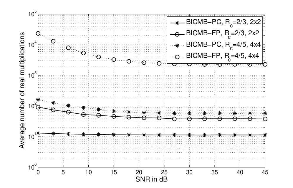
In order to measure the decoding complexity, the average number of real multiplications which are the most expensive operations in terms of machine cycles, for acquiring one bit metric is calculated at different SNR for BICMB-PC and BICMB-FP, respectively. In [30], [31], an efficient reduced complexity decoding technique was introduced for BICMB-FP, which is applied in this paper. For fair comparisons, a similar decoding technique is applied to BICMB-PC. Fig. 4 shows the complexity comparisons for BICMB-PC and BICMB-FP in dimensions of $2$ and $4$ using $64$-QAM. For the dimension of $2$, the complexity of BICMB-PC is $0.8$ and $0.5$ orders of magnitude lower than BICMB-FP at low and high SNR respectively. In the dimension of $4$ case, the improvements reach $2.2$ and $1.6$ orders of magnitude.

Additionally, Fig. 5 shows the complexity comparisons for uncoded full-diversity full-multiplexing SVD systems of FPMB and PCMB in dimensions of $2$ and $4$ using $64$-QAM. In [30], [32], an efficient reduced complexity SD technique was introduced, which is applied in this paper. For the dimension of $2$, the complexity of GCMB is $0.5$ order of magnitude lower than FPMB at low SNR and similar to FPMB at high SNR. In the dimension of $4$ case, the complexity of GCMB is $1.7$ orders of magnitude lower than FPMB at low SNR and similar to FPMB at high SNR. Fig. 4 and Fig. 5 show that the complexity reduction from BICMB-FP to BICMB-PC is greater than the reduction from FPMB to PCMB achieved in [22] for dimensions $2$ and $4$.

In this paper, BICMB-PC which combines PSTBC and multiple beamforming technique is proposed. It is a new technique with both full diversity and full multiplexing for convolutional coded SVD-MIMO systems. Diversity analysis and decoding complexity analysis are provided. It is shown that BICMB-PC achieves a similar BER performance to BICMB-FP, which is also a full-diversity full-multiplexing technique for convolutional coded SVD-MIMO systems. Particularly, for dimensions $2$ and $4$, because only one of the real or imaginary part of the received signal is required to calculate one bit metric for the Viterbi decoder, the worst-case decoding complexity of $\mathcal{O}(M^{\frac{D}{2}}-0.5)$ for BICMB-PC is much lower than $\mathcal{O}(M^{D}-1)$ for BICMB-FP, which provides the advantage of BICMB-PC. Compared to the uncoded system, the complexity reduction from BICMB-FP to BICMB-PC is greater than the reduction from FPMB to PCMB achieved in [22] for dimensions $2$ and $4$. Furthermore, since the precoded part of BICMB-PP could be considered as a smaller dimensional BICMB-FP, BICMB-PC of dimensions $2$ and $4$ could be applied to replace the precoded part and reduce the complexity for BICMB-PP.

References

- [1] A. Paulraj, R. Nabar, and D. Gore, Introduction to Space-Time Wireless Communication. Cambridge University Press, 2003.
- [2] L. Zheng. and D. Tse, “Diversity and Multiplexing: a Fundamental Tradeoff In Multiple-antenna Channels,” IEEE Trans. Inf. Theory, vol. 49, no. 5, pp. 1073–1096, May 2003.
- [3] H. Jafarkhani, Space-Time Coding: Theory and Practice. Cambridge University Press, 2005.
- [4] E. Sengul, E. Akay, and E. Ayanoglu, “Diversity Analysis of Single and Multiple Beamforming,” IEEE Trans. Commun., vol. 54, no. 6, pp. 990–993, Jun. 2006.
- [5] E. Akay, E. Sengul, and E. Ayanoglu, “Bit-Interleaved Coded Multiple Beamforming,” IEEE Trans. Commun., vol. 55, no. 9, pp. 1802–1811, Sep. 2007.
- [6] E. Akay, H. J. Park, and E. Ayanoglu. (2008) On ”Bit-Interleaved Coded Multiple Beamforming”. arXiv: 0807.2464. [Online]. Available: http://arxiv.org
- [7] H. J. Park and E. Ayanoglu, “Diversity Analysis of Bit-Interleaved Coded Multiple Beamforming,” in Proc. IEEE ICC 2009, Dresden, Germany, Jun. 2009.
- [8] ——, “Diversity Analysis of Bit-Interleaved Coded Multiple Beamforming,” IEEE Trans. Commun., vol. 58, no. 8, pp. 2457–2463, Aug. 2010.
- [9] S. K. Mohammed, E. Viterbo, Y. Hong, and A. Chockalingam, “Precoding by Pairing Subchannels to Increase MIMO Capacity with Discrete Input Alphabets,” IEEE Trans. Inf. Theory, vol. 57, no. 7, pp. 4156–4169, Jul. 2011.
- [10] ——, “MIMO Precoding with X- and Y-Codes,” IEEE Trans. Inf. Theory, vol. 57, no. 6, pp. 3542–3566, Jun. 2011.
- [11] H. J. Park and E. Ayanoglu, “Constellation Precoded Beamforming,” in Proc. IEEE GLOBECOM 2009, Honolulu, HI, USA, Nov. 2009.