Restricted Linear Constrained Minimization of quadratic functionals
Abstract
In this work a linearly constrained minimization of a positive semidefinite quadratic functional is examined. Our results are concerning infinite dimensional real Hilbert spaces, with a singular positive operator related to the functional, and considering as constraint a singular operator. The difference between the proposed minimization and previous work on this problem, is that it is considered for all vectors perpendicular to the kernel of the related operator or matrix.
Keywords: Quadratic functional, Constrained Optimization,
Moore-Penrose inverse , Restricted Optimization.
2010 Mathematics Subject Classification: 47A05, 47N10, 15A09.
1 Introduction
The quadratic programming problem with equality
constraints is one of the basic problems in optimization, in both
the finite and the infinite dimensional case. The general problem is
to locate from within a given subset of a vector space the
particular vector which minimizes a given functional. In this case,
the subset of vectors is defined by a set of linear constraint
relations and the functional is quadratic. In a classical book of
Optimization Theory by Luenberger [7], various similar
optimization problems are presented, for both finite and infinite
dimensions.
In the field of applied mathematics, a strong interest
is shown in applications of the generalized inverse of matrices or
operators. Generalized inverses can be used whenever a matrix/
operator is singular, in many fields of both computational and also
theoretical aspects. An application of the Moore-Penrose inverse in
the finite dimensional case, is the minimization of a positive
definite quadratic functional under linear constraints, presented in
Manherz and Hakimi [8].
The problem studied in their work in
the following:
where and is a
positive definite matrix.
In this work we will extend this result
for positive semidefinite matrices or operators acting on infinite
dimensional real Hilbert spaces. Since in this case the operator
studied is singular, the proposed minimization is attained for the
vectors perpendicular to the kernel of the operator (or matrix) of
the quadratic functional.
2 Preliminaries and notation
The notion of the generalized inverse of a matrix was first introduced by H. Moore in 1920, and again by R. Penrose in 1955. These two definitions are equivalent and the generalized inverse of an operator or matrix is also called the Moore- Penrose inverse. It is known that when is singular, then its unique generalized inverse (known as the Moore- Penrose inverse) is defined. In the case when is a real matrix, Penrose showed that there is a unique matrix satisfying the four Penrose equations, called the generalized inverse of , noted by . The generalized inverse, known as Moore-Penrose inverse, of an bounded linear operator with closed range, is the unique operator satisfying the following four conditions:
| (1) |
where denotes the adjoint operator of .
In what follows, we consider
a separable infinite dimensional Hilbert space, denotes the set of all bounded operators on
and all operators mentioned are supposed to have
closed range. In addition, will denote the range of
an operator , and will denote its kernel.
It is
easy to see that ,
is the orthogonal projection of onto
, denoted by , and that is the
orthogonal projection of onto noted by . It is well known that
.
It is also known that
is bounded if and only if has a closed range.
If
has a closed range and commutes with , then is
called an EP operator. EP operators constitute a wide class of
operators which includes the self adjoint operators, the normal
operators and the invertible operators.
Let us consider the equation , where is singular. If , then
the equation has no solution. Therefore, instead of trying to solve
the equation , we may look for a vector that
minimizes the norm . Note that the vector is unique.
In this case we consider the equation , where
is the orthogonal projection on .
The following two propositions can be found in [5] and hold for operators and matrices:
Proposition 2.1
Let and . Then, for , the following are equivalent:
- (i)
- (ii)
- (iii)
Let . This set of solutions is closed and convex, therefore, it has a unique vector with minimal norm. In the literature (eg. Groetsch [5]), is known as the set of the generalized solutions.
Proposition 2.2
Let and , and the equation . Then, if is the generalized inverse of , we have that , where is the minimal norm solution defined above.
This property has an application in the problem of minimizing a
symmetric positive definite quadratic functional subject to linear
constraints, assumed consistent.
As mentioned above, EP operators
include normal and self adjoint operators, therefore the operator
in the quadratic form studied in this work is EP. An operator
with closed range is called EP if
. It is easy to see that
| (2) |
We take advantage of the fact that EP operators
have a simple canonical form according to
the decomposition . Indeed an EP operator has the following simple
matrix form, ,
where the operator is
invertible, and its generalized inverse has the form
(see [2], [4] ).
In the finite dimensional case, if and , the unitary matrix has the form
where is an orthonormal basis for
the column space of and is an orthonormal basis for the
null space of the matrix . In Matzakos and Pappas [9] an
algorithm is presented for the symbolic computation of the
Moore-Penrose inverse for EP matrices and the corresponding
factorization is presented.
As mentioned
above, a necessary condition for the existance of a bounded
generalized inverse is that the operator has closed range.
Nevertheless, the range of the product of two operators with closed
range is not always closed. In Izumino [6] an equivalent
condition is given, using orthogonal projections :
Proposition 2.3
Let and be operators with closed range. Then, has closed range if and only if has closed range.
We will use the above theorem to prove the existence of the Moore- Penrose inverse used in our work.
3 The Generalized inverse in linear constrained minimization
The Generalized inverse of an operator or matrix plays a crucial role in many optimization problems where minimal norm solutions are studied. Ben-Israel and Greville ([1] chapter 3), and Campbell and Meyer ([2] chapter 3.6), have considered the constrained least- squares problem
with all complex.
In Chen [3],
a similar problem is considered using partial ordering induced by
cones, where the generalized inverse plays a fundamental role.
The
purpose of this paper is to extend the work done on this subject by
Manherz and Hakimi [8]. At first we will extend the finite
dimensional results in the case of positive definite operators, and
then we will examine the case when the operator is singular.
3.1 Positive Definite Quadratic Forms
Let be a positive definite symmetric matrix. The following theorem can be found in Manherz and Hakimi [8] :
Theorem 3.1
Let Q be positive definite. Consider the equation .
If the set is not empty, the the
problem :
and p, a arbitrary has the unique solution
A generalization of the above theorem for infinite dimensional Hilbert spaces, is by replacing with an invertible positive operator . The operator must be singular, otherwise this problem is trivial. In the case of operators instead of matrices, the proof is similar to Manherz and Hakimi [8], but the existence of a bounded Moore- Penrose inverse is not trivial like in the finite dimensional case.
Lemma 3.2
Let be an invertible positive
operator with closed range
and
singular with closed range.
Then, the range of
is closed , where denotes the operator
.
Therefore, the expression of the above theorem in infinite dimensional Hilbert spaces is the following:
Theorem 3.3
Let be positive definite and the equation , where is singular.
If the set is not empty, the the
problem :
with arbitrary has the unique solution
3.2 Positive Semidefinite Quadratic Forms
An interesting case to examine, is when the positive operator is singular, that is, is positive semidefinite. In this case, since , we have that for all and so, when this problem will take the form
which is usually treated using the simplex method,
when the space is finite dimensional.
A different approach in both the finite and infinite dimensional
case would be to look among the vectors for a minimizing vector for
. In other words, we will look for the minimum of
under the constraints
Using the fact that is an operator, we
will make use of the following proposition that can be found in
Drivaliaris et al [4]:
Proposition 3.4
Let with closed range.
Then the following are equivalent:
i) is EP.
ii) There exist
Hilbert spaces and ,
unitary and isomorphism such that
We present a sketch of the proof for (1)(2):
Proof. : Let , , with
for all and , and Since is EP, and thus is unitary. Moreover it is easy to see that for all . It is obvious that is an isomorphism. A simple calculation shows that
It is easy to see that when and is
positive, so is , since .
In what follows,
will denote a singular positive operator with a canonical form
, is the unique solution of the equation
and
Theorem 3.5
Let T be positive semidefinite and . Consider the equation .
If the set is not empty, then the
problem :
and p, a arbitrary has the unique solution
assuming that the operator has closed range.
Proof. : Since we will restrict the minimization for all vectors we have that , where for all vectors , according to the decomposition
Let with and
arbitrary and not a function of . Hence, the vector
that minimizes also minimizes
We can easily see that
and that
Set , which implies
that .
We have that
Hence,
and so, since
Since , we have that and therefore, the minimal norm solution is
By substitution, we have that
and
since for all
The only thing that needs to be proved is the fact that the
operator has closed range and so its Moore-Penrose
Inverse is bounded. Since the two operators and are
arbitrary, one does not expect that the range of their product will
always be closed. From Proposition 2.3, this is equivalent to
the fact that the operator has closed range because
and the proof is completed. In the sequel, we present an example which clarifies Theorem 3.5. In addition, the difference between the proposed minimization () and the minimization for all is clearly indicated.
Example 3.6
Let , and the positive semidefinite matrix
We are looking for the minimum of the functional
with and the set of constraints S is defined as
The set
has the form .
With easy computations, we can see that all
vectors satisfying the constraint , where and , have the form
The matrices are
Using theorem 3.5 we can see that the minimizing vector of under
is
The
minimum value of is then equal to 1.4175
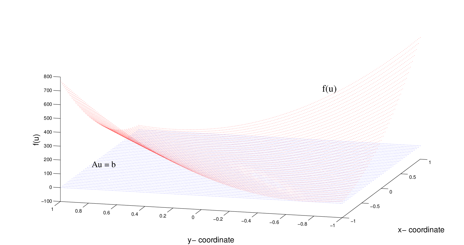
In Figure 1 we can clearly see that the minimization of the
functional for all vectors
having the form , belonging
to the plane , is attained.
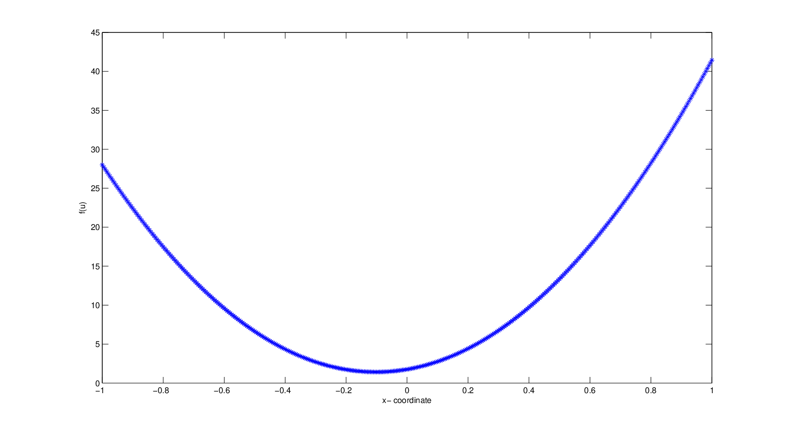
In Figure 2 we can see
that among all vectors belonging to
satisfying , having the form , the vector found from Theorem 3.5
minimizes the functional .
We will also examine the minimization of in the cases when and when , given that , so that the difference between them is clearly indicated:
-
When the minimization takes place for all vectors , then this problem takes the form : minimize .
We can see with easy calculations, that the only vector is . In this case , -
When the minimization takes place for all vectors , then the minimizing vector of is and the minimum value of is .
Corollary 3.7
We can easily see that, in the case when the vectors are both
equal to zero, the functional is a constrained quadratic form
under .
In this case, the
minimizing vector belonging to is
then equal to as it was
discussed and proved in [10].
4 Conclusions
In this work, we propose a constrained minimization in the case of a quadratic functional related to a positive semidefinite operator. The proposed minimization takes place for all vectors perpendicular to the kernel of the corresponding operator. This proposed constrained minimization method has the advantage of a unique solution and is easy to implement. Practical importance of this result in the finite dimensional case, can be in numerous applications such as network analysis, filter design, spectral analysis, direction finding etc. In many of these cases, the knowledge of the non zero part of the solution corresponding to the matrix may be of importance.
References
- [1] Ben-Israel A., Grenville T. N. E., Generalized Inverses: Theory and Applications, Springer- Verlag, Berlin (2002).
- [2] Campbell S. L., Meyer C. D. : Generalized inverses of Linear Transformations, Dover Publ. New York (1979).
- [3] Chen, Y. Nonnegative definite matrices and their applications to matrix quadratic programming problems, Linear Multilinear Alg., 33, pp.189- 201 (1993)
- [4] Drivaliaris D., Karanasios S., Pappas D. , Factorizations of EP operators, Linear Algebra and Applications, 429, pp. 1555-1567, (2008)
- [5] Groetsch C. : Generalized inverses of linear operators, Marcel Dekker Inc., New York (1977)
- [6] Izumino S., The product of operators with closed range and an extension of the reverse order law, Tohoku Mathematical Journal, 34, pp. 43–52.(1982)
- [7] Luenberger D., Optimization by Vector Space Methods, Wiley Publ. New York. (1969)
- [8] Manherz R. K., Hakimi S. L : The Generalized Inverse in Network Analysis and Quadratic- Error Minimization Problems, IEEE Trans. Circuit Theory, pp. 559- 562, (1969)
- [9]
Matzakos N., Pappas D., EP Matrices: Computation of the Moore- Penrose Inverse via
factorizations. Journal of Applied Mathematics and Computing, (2010-
to appear)
doi: 10.1007/s12190-009-0311-0 - [10] Pappas D, Minimization of Constrained Quadratic forms in Hilbert Spaces, preprint, http://arxiv.org/abs/1003.5676, [math.FA] (2010)