A Lower Bound on the Estimator Variance
for the Sparse Linear ModelThanks: This work was supported by the FWF under Grants S10602-N13 (Signal and Information Representation) and S10603-N13 (Statistical Inference) within the National Research Network SISE, by the Israel Science Foundation under Grant 1081/07, and by the European Commission under the FP7 Network of Excellence in Wireless COMmunications NEWCOM++
(contract no. 216715).
Sebastian SchmutzhardAlexander JungAffiliation: Institute of Communications and Radio-Frequency Engineering, Vienna University of TechnologyA-1040 Vienna, Austria; e-mail: {ajung, fhlawats}@nt.tuwien.ac.at
Franz HlawatschAffiliation: Institute of Communications and Radio-Frequency Engineering, Vienna University of TechnologyA-1040 Vienna, Austria; e-mail: {ajung, fhlawats}@nt.tuwien.ac.at
Zvika Ben-HaimYonina C. EldarAffiliation: Technion—Israel Institute of TechnologyHaifa 32000, Israel; e-mail: {zvikabh@tx, yonina@ee}.technion.ac.il
Affiliation: NuHAG, Faculty of Mathematics, University of ViennaA-1090 Vienna, Austria; e-mail: sebastian.schmutzhard@univie.ac.at
Abstract
We study the performance of estimators of a sparse nonrandom vector based on an observation which is linearly transformed and corrupted by
additive
white Gaussian noise.
Using the reproducing kernel Hilbert space framework, we derive
a new lower bound on the estimator variance for a given differentiable bias function (including the unbiased case) and an almost arbitrary transformation matrix (including the
underdetermined case considered in compressed sensing theory). For the special case of a sparse vector corrupted by white Gaussian noise—i.e., without a linear transformation—and
unbiased estimation, our lower bound improves on previously proposed bounds.
We study the problem of estimating a nonrandom parameter vector
which is
sparse, i.e., at most of its entries are nonzero, where (typically ). We thus
have
(1)
where denotes the number of nonzero entries of .
While the sparsity degree is assumed to be known, the set of positions of the nonzero entries of (denoted by ) is unknown. The estimation of is based on the observed vector
given
by
(2)
with a known
system matrix and white Gaussian noise
with known variance . The matrix is arbitrary except that it is assumed to satisfy the standard
requirement
(3)
where denotes the minimum number of linearly dependent columns of [1].
The observation
model (2) together with (1) will be referred to as the
sparse linear model (SLM).
Note that we also allow
(this case is relevant to compressed sensing methods [2, 1]);
however, condition (3) implies that .
The case of correlated Gaussian noise with a known nonsingular correlation matrix can be reduced to the SLM by means of a noise whitening transformation.
An important special case of the SLM is given by (so that ),
i.e.,
(4)
where again and . This will be referred to as the sparse signal in noise model (SSNM).
Lower bounds on the estimation variance for the SLM have been studied previously.
In particular, the Cramér–Rao bound (CRB) for the SLM was derived in [3].
For the SSNM (4), lower and upper bounds on the minimum variance of unbiased estimators were derived in [4].
A problem with the lower bounds of [3] and [4] is the fact that they
exhibit a discontinuity when passing from the case to the case .
In this paper, we use the mathematical framework of reproducing kernel Hilbert spaces (RKHS) [5, 6, 7]
to derive a novel lower variance bound for the SLM.
The RKHS framework allows pleasing geometric interpretations of existing bounds, including the CRB, the Hammersley-Chapman-Robbins bound [8],
and the Barankin bound [9].
The bound we derive here holds for estimators with a given differentiable bias function.
For the SSNM, in particular, we obtain a lower bound for unbiased estimators
which is tighter
than the bounds in [4] and, moreover, everywhere continuous. As we will show, RKHS theory relates the
bound for the SLM to that obtained for the
linear model without a sparsity assumption. We note that the RKHS framework has been previously applied to estimation [6, 7] but,
to the best of our knowledge, not to the SLM.
This paper is organized as follows.
In Section II, we review some fundamentals of parameter estimation.
Relevant elements of RKHS theory are summarized in Section III.
In Section IV, we use RKHS theory to derive a lower variance bound for the SLM.
Section V considers the special case of unbiased estimation within the SSNM.
Section VI presents a numerical comparison of the new bound with the variance of two established estimation schemes.
II Basic Concepts
We first review some basic concepts of parameter estimation [10]. Let be the nonrandom parameter vector to be estimated,
the observed vector, and the probability density function (pdf) of ,
parameterized by . For the SLM, as defined in (1) and
(5)
II-AMinimum-Variance Estimators
The estimation error incurred by an estimator can be quantified by the mean squared error (MSE)
,
where the notation indicates that the expectation is taken with respect to the pdf parameterized by .
Note that
depends on the true parameter value, . The MSE can be decomposed as
(6)
with the estimator bias
and the estimator variance
.
A standard approach to defining an optimum estimator is to fix the bias, i.e.,
for all ,
and minimize the variance for all under this bias constraint.
However, in many cases, such a “uniformly optimum” estimator does not exist. It is then natural to consider “locally optimum” estimators
that minimize only at a given parameter value .
This approach is taken here. Note that it follows from (6) that once the bias is fixed, minimizing the variance is equivalent to minimizing the MSE .
The bias constraint can be equivalently written as the mean constraint
Thus, we consider the constrained optimization problem
(7)
where
The minimum variance achieved by the locally optimum estimator at will be denoted as
This is also known as the Barankin bound (for the prescribed mean ) [9].
Using RKHS theory, it can be shown that exists, i.e., there exists a unique minimum for (7), provided that there exists at least one estimator with mean for all and finite variance at (see also Section III).
For unbiased estimation, i.e.,
, is called a locally minimum variance unbiased (LMVU) estimator.
Unfortunately, is difficult to compute in many cases, including the case of the SLM. Lower bounds on
are, e.g., the CRB and the Hammersley-Chapman-Robbins bound [8].
Let , ,
and denote the th
entries of , ,
and , respectively.
We have
with
.
Thus,
(7) is equivalent to the scalar optimization problems
(8)
where
The minimum variance achieved by at is denoted as
(9)
II-BCRB of the Linear Gaussian Model
In our further development, we will make use of the CRB for the linear Gaussian model (LGM) defined by
(10)
with the nonrandom parameter (not assumed sparse),
theobservation , the known matrix ,
and white Gaussian noise .
As before, we assume that ; furthermore, we assume that has full column rank, i.e.,
is nonsingular.
The relationship of this model with the SLM, as well as the different notation and different dimension ( instead of ),
will become clear in Section IV.
Consider estimators of the th parameter component whose bias is equal to some prescribed differentiable function ,
i.e., or equivalently
with ,
for all . Let denote the minimum variance achievable by such estimators at a given true parameter .
The CRB is the following lower bound on the minimum variance [10]:
(11)
where
,
i.e., is the vector of dimension whose th entry is .
We note that if is an affine function of .
In particular, this includes the unbiased case ().
III The RKHS Framework
In this section, we review some RKHS fundamentals which will provide a basis for our further development.
Consider a set
(not necessarily a linear
space) and a positive
semidefinite111
That is, for any finite set with , the matrix with entries is positive
semidefinite. “kernel” function .
For each fixed , the function maps into .
The RKHS is a Hilbert space of functions which is defined as the
closure of the linear span of the set of functions .
This closure is taken with respect to the topology given by the scalar product which is defined via the reproducing property [5]
This relation holds for all and .
The associated norm is given by
.
We now consider the constrained
optimization problem (8) for a given mean function (formerly denoted by ; we temporarily
drop the subscript for better readability). According to [6, 7], for certain classes of parametrized pdf’s
(which include the Gaussian pdf in (5)),
one can associate with this optimization problem an RKHS
whose kernel is given by
It can be shown [6, 7] that
if and only if there exists at least one estimator with mean for all and finite variance at . Furthermore, under this condition, the minimum variance
in (9) is finite and
allows the following expression involving the norm
:
(12)
This is an RKHS formulation of the Barankin bound. Unfortunately, the norm
is often difficult to compute.
For the SLM in (2), (1), (5),
; the kernel here is a mapping which is easily shown to be given
by
(13)
where . An RKHS can also be defined for the LGM in (10). Here, ,
and the kernel with is
a mapping given by
(14)
Note that these kernels differ in their domain, which is for
and for .
IV A Lower Bound on the Estimator Variance
We now continue our treatment of the SLM estimation problem.
In what follows, will be understood to denote the bias-constrained minimum
variance
(9) specifically for the SLM. This means, in particular, that , and hence the set of admissible
estimators is given by
(15)
We will next
derive a lower bound on .
IV-ARelaxing the Bias Constraint
The first step in this derivation is to relax the bias constraint .
Let be a fixed set of different indices (not related to ),
and let
Clearly, ; however, contrary to ,
is a linear subspace of .
Let be the set of all
estimators with mean for all
(but not necessarily for all ),
i.e.,
Let us now consider the minimum variance among all estimators in , i.e.,
(16)
Because is a less restrictive constraint than
used in the definition of , we have
(17)
i.e., is a lower bound on .
A closed-form expression of appears to be difficult to obtain in the general case, because
in general.
Therefore, we will use RKHS theory to derive a lower bound on .
IV-BTwo Isometric RKHSs
An RKHS
for the SLM can also be defined on , using a kernel
that is given by
the right-hand side of (13) but whose arguments are assumed to be in
and not just in (however, recall that in general).
This RKHS will be denoted . The minimum variance
in (16) can then be expressed as (cf. (12))
(18)
In order to develop this expression, we define some notation.
Consider an
index set .
We denote by the
submatrix of our
matrix
whose th column is given by the th column of . Furthermore, for a vector ,
we denote by the subvector whose th entry is the th entry of .
We now introduce a second RKHS. Consider the LGM in (10) with
matrix ,
and let with denote the RKHS for that LGM as defined by the kernel in (14).
Exploiting the linear-subspace structure of , it can be shown that our RKHS for a given
is isometric to with chosen as
(19)
Here, is the pseudo-inverse of (recall that , and note that
is guaranteed to exist because of our assumption (3)).
More specifically, the isometry mapping each to an
is given by
(20)
where
(21)
Here, is the orthogonal projection matrix on the range of .
The factor can be interpreted as a
measure of the distance between the point and the subpsace
associated with the index set . We can write (20) as
where denotes the for which
(i.e., the entries of appear in at the appropriate positions within ,
and the remaining entries of are zero).
Consider now the image of
under the mapping ,
(22)
Since is an isometry, we have .
Combining this identity with (18), we obtain
(23)
IV-CLower Bound on
We will now use expression (23) to derive a lower bound on in terms of the CRB for the LGM in (11).
Consider the minimum estimator variance for the LGM under the constraint of the prescribed mean function ,
,
still for and for given by (19).
We have (cf. (12))
To summarize, we have the following chain of lower bounds on the bias-constrained variance at :
(28)
While is the loosest of these bounds, it is attractive because
of its closed-form expression in (26) (together with (27) and (19)).
We note that the inequality (24) becomes an equality if is an affine function of ,
or equivalently (see (22)), if is an affine function of .
In particular, this includes the unbiased case
().
Recalling that
(we now reintroduce the subscript ),
a lower bound on is obtained from (28)
as
For a high lower bound, the index sets should in general be chosen such that the respective factors in (26)
are large. (This means that the “distances” between and are small, see (21).)
Formally using the optimum for each , we arrive at the main result of this
paper.
Theorem. Let be an estimator for the SLM (2), (1)
whose mean equals for all . Then the variance of
at a given parameter vector
satisfies
(29)
where ,
with given by (26) together with (27) and (19).
V Special Case: Unbiased Estimation for the SSNM
The SSNM in (4) is a special case of the SLM with .
We now consider unbiased estimation (i.e., ) for the SSNM.
Since an unbiased estimator with uniformly minimum variance does not exist [4],
we are interested in
a lower variance bound at a fixed
.
We denote by and the value and index, respectively,
of the -largest (in magnitude) entry of ; note that this is the
smallest (in magnitude) nonzero entry of if , and zero if .
Consider an unbiased estimator .
For ,
using the lower bound in (26)
with any index set of size such that ,
one can show that
(30)
This bound is actually the minimum variance (i.e., the variance of the LMVU estimator)
since it is achieved by the specific unbiased estimator (which is the LMVU estimator for ).
On the other hand, for , the lower bound
with can be shown to lead to the
inequality
(31)
Combining (30) and (31), a lower bound on the overall variance
is obtained as
(32)
Thus, recalling that for unbiased estimators, we arrive at the following
result.
Corollary. Let be an unbiased estimator for the SSNM in (4). Then the MSE of
at a given
satisfies
(33)
This lower bound
is tighter (i.e., higher) than the lower bound derived in [4].
Furthermore, in contrast to the bound in [4], it is a function of that is everywhere continuous. This fact is theoretically pleasing since the
MSE of any estimator is a continuous function of [11].
Let us consider the special case of
. Here, and are simply the value and index, respectively, of the single nonzero entry of .
Using RKHS theory, one can show that the estimator given componentwise by
with ,
is the LMVU estimator at . That is, the estimator is unbiased and its MSE achieves the lower bound (33).
This also means that (33) is actually the minimum MSE (achieved by the LMVU estimator).
While is not very practical since it explicitly involves the unknown true parameter , its existence demonstrates the tightness of the bound
(33).
VI Numerical Results
For the
SSNM in (4),
we will compute the lower variance
bound
(see (29)) and compare it with the
variance of two established estimators, namely, the maximum likelihood (ML) estimator and the hard-thresholding (HT) estimator.
The ML estimator is given by
where the operator retains the largest (in magnitude) entries and zeros out
all others. The HT estimator is given
by
(34)
where is a fixed threshold.
For simplicity, we consider the SSNM for .
In this case, the bound (29) can be shown to
be
(35)
where , is any index different from (it can be shown that all such indices equally maximize
the lower bound), , and .
(We note that (35) simplifies to (32) for the special case of an unbiased estimator.)
Since we
compare the bound (35) to the ML and HT estimators, is set equal to the
mean of the respective estimator (ML or HT).
For a numerical evaluation, we generated parameter vectors with , , , and different .
(The fixed choice is justified by the fact that neither the variances of the ML and HT estimators nor the corresponding variance bounds depend on .)
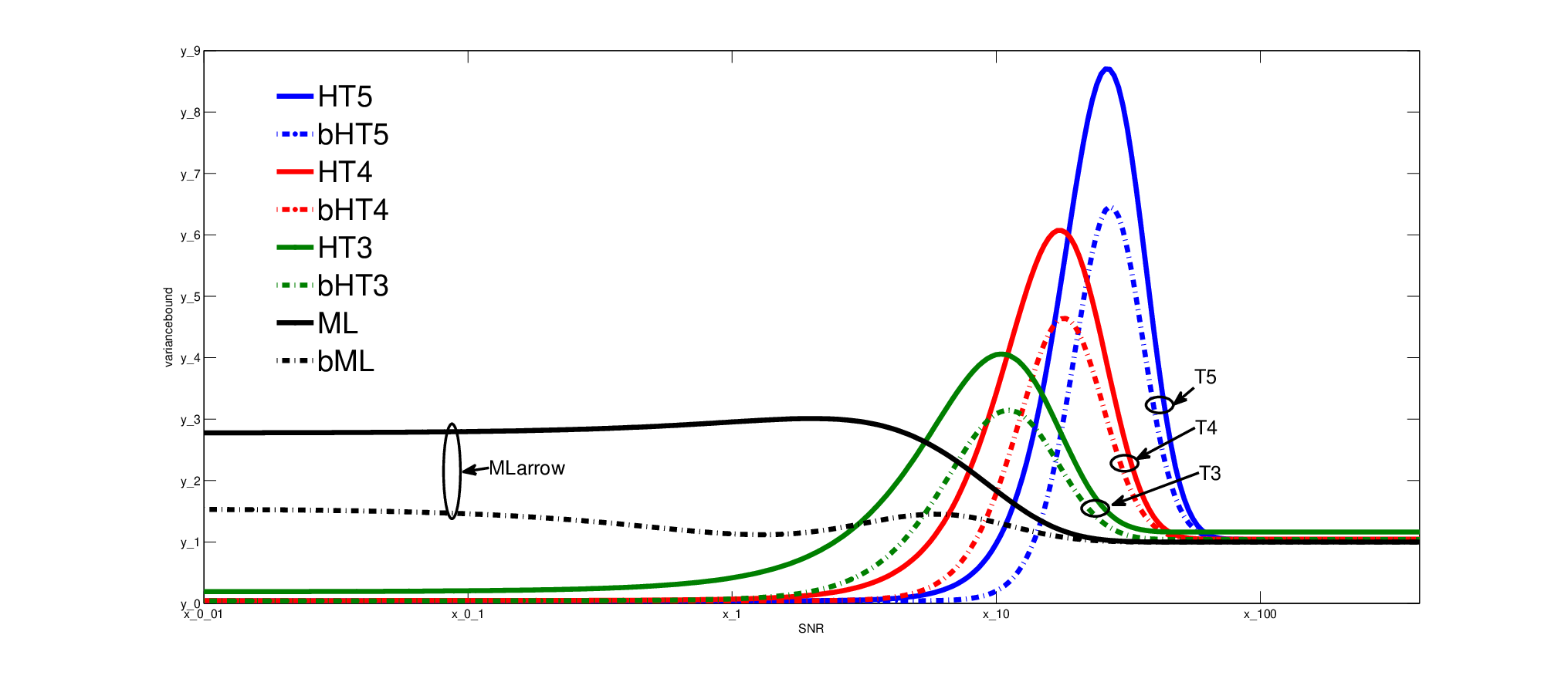
In Fig. 1, we plot the variances and
(the latter for three different choices of
in (34)) along with the corresponding bounds (35), as a function of the signal-to-noise ratio (SNR)
. It is seen that for SNR larger than about 18 dB, all variances and bounds are effectively equal (for the HT estimator,
this is true if is not too small). However, in the medium-SNR
range, the variances of the ML and HT estimators are significantly higher than
the corresponding lower bounds.
We can conclude that there might exist estimators with the same mean as that of the ML or HT estimator but smaller variance.
Note, however, that a positive statement regarding the existence of such estimators cannot be based on our analysis.
Figure 1: Variance of the ML and HT estimators and corresponding lower bounds versus the SNR ,
for the SSNM
with and .
VII Conclusion
Using the mathematical framework of reproducing kernel Hilbert spaces,
we derived a novel lower bound on the variance of estimators
of a sparse vector under a bias constraint. The observed vector was assumed to be a linearly transformed and noisy version of the sparse vector to be estimated.
This setup includes the underdetermined case relevant to compressed sensing. In the special case of unbiased estimation of a noise-corrupted sparse vector,
our bound improves on the best known lower bound. A comparison
with the variance of two established estimators
showed that there might exist estimators with the same bias
but a smaller variance.
References
[1]
J. A. Tropp, “Greed is good: Algorithmic results for sparse approximation,”
IEEE Trans. Inf. Theory, vol. 50, pp. 2231–2242, Oct. 2004.
[2]
D. L. Donoho, “Compressed sensing,” IEEE Trans. Inf. Theory, vol. 52,
pp. 1289–1306, April 2006.
[3]
Z. Ben-Haim and Y. C. Eldar, “The Cramér–Rao bound for estimating a
sparse parameter vector,” IEEE Trans. Signal Processing, vol. 58,
pp. 3384–3389, June 2010.
[4]
A. Jung, Z. Ben-Haim, F. Hlawatsch, and Y. C. Eldar, “On unbiased estimation
of sparse vectors corrupted by Gaussian noise,” in Proc. IEEE
ICASSP-2010, (Dallas, TX), pp. 3990–3993, March 2010.
[5]
N. Aronszajn, “Theory of reproducing kernels,” Trans. Am. Math. Soc.,
vol. 68, pp. 337–404, May 1950.
[6]
E. Parzen, “Statistical inference on time series by Hilbert space methods,
I.,” Tech. Rep. 23, Appl. Math. Stat. Lab., Stanford University, Stanford,
CA, Jan. 1959.
[7]
D. D. Duttweiler and T. Kailath, “RKHS approach to detection and estimation
problems – Part V: Parameter estimation,” IEEE Trans. Inf.
Theory, vol. 19, pp. 29–37, Jan. 1973.
[8]
J. D. Gorman and A. O. Hero, “Lower bounds for parametric estimation with
constraints,” IEEE Trans. Inf. Theory, vol. 36, pp. 1285–1301, Nov.
1990.
[9]
E. W. Barankin, “Locally best unbiased estimates,” Ann. Math. Statist.,
vol. 20, no. 4, pp. 477–501, 1949.
[10]
S. M. Kay, Fundamentals of Statistical Signal Processing: Estimation
Theory.
Englewood Cliffs, NJ: Prentice Hall, 1993.
[11]
E. L. Lehmann and G. Casella, Theory of Point Estimation.
New York: Springer, 2003.