跳到论文正文
W Papers独立论文阅读器 arXiv:1009.3008 论文正文 计算阅读时间 · 0%
引用这篇论文根据当前论文元数据生成,正式投稿前建议核对。


License: arXiv.org perpetual non-exclusive license
arXiv:1009.3008v2 [cond-mat.soft] 28 Apr 2011

Smoluchowski Dynamics and the Ergodic-Nonergodic Transition

Gene F. Mazenko Affiliation: The James Franck Institute and the Department of Physics
The University of Chicago
Chicago, Illinois 60637, USA

Abstract

We use the recently introduced theory for the kinetics of systems of classical particles to investigate systems driven by Smoluchowski dynamics. We investigate the existence of ergodic-nonergodic (ENE) transitions near the liquid-glass transition. We develop a self-consistent perturbation theory in terms of an effective two-body potential and work to second order in this potential. At second order, we have an explicit relationship between the static structure factor and the effective potential and choose the static structure factor in the case of hard spheres to be given by the solution of the Percus-Yevick approximation for hard spheres. Then, using the analytically determined ENE equation for the ergodicity function, we find an ENE transition for packing fraction η\eta greater than a critical value η∗=0.76\eta^{*}=0.76 which is physically unaccessible. The existence of a linear fluctuation-dissipation theorem in the problem is shown and used to great advantage.

I Introduction

We continue[1] our presentation of a self-consistent approach to the kinetics of classical systems of particles by studying the fluctuations in equilibrium of a system driven by Smoluchowski dynamics. We first show that the system obeys a linear fluctuation-dissipation theorem (FDT). This simplifies the structure of the theory significantly giving the conventional linear relation between the density-density correlation function and the conjugate response function. We present here a perturbation theory valid to second order in an effective interaction potential. Because of the self-consistency we are able to show that this expansion is useful even for systems with hard-core interactions.

This approach was demonstrated at first order in Ref. 1 (henceforth referred to as FTSPD) where the effective potential is found to be proportional to the direct correlation function. Here we extend the calculation to second order. In this paper we focus on the collective (or Ornstein-Zernike) second order self-energies. We show that these self-energies are quadratic functionals of the full density-density correlation functions, the components of the self-energies individually satisfy a FDT, no wave-number or frequency cut offs are needed[2], and the set of Dyson equations fundamental to the theory can be replaced by a single-kinetic equation of the same form as that produced in memory-function theories [3, 4].

Going further, one can show that the collective contribution, again using the FDT, gives a relation for the static structure which agrees with the result from a purely static calculation giving the structure factor in terms of the direct correlation function and the direct correlation function self-consistently in terms of the static structure factor. Our approach is to assume the static structure factor is known and to solve for that effective potential which satisfies the second order structural equation. This effective potential is then available in the dynamical calculations. It could also be used in other static calculations. We focus here primarily on the large wavenumber regime near the structure factor maximum.

We also show that it is only the collective part of the self-energy which enters into the determination of the ergodic-nonergodic (ENE) phase-diagram. The ENE transition occurs when the density-density correlation develops a zero-frequency δ\delta function. The amplitude of this δ\delta function satisfies a nonergodicity equation. This equation is very similar to that found[5] in mode-coupling theory (MCT). For a system characterized by a structure factor obtained as the solution of the Percus-Yevick approximation[6] for hard-spheres we find a transition at packing fraction η∗=0.76\eta^{*}=0.76. Conventional MCT gives η=0.51\eta=0.51. As obtained here, η∗\eta^{*} is well above any physically attainable density in agreement with experiment and simulation. If we drop self-consistency and use the first order effective potential in determining η∗\eta^{*} we obtain the value η∗=0.60\eta^{*}=0.60 even though the first and second order effective potentials are very similar. Therefore η∗\eta^{*} is a rather sensitive quantity. Despite our prejudices that there is no physical ENE transition in the single-component hard-sphere Smoluchowski dynamics, more work checking perturbations to our solution is required before one can claim a “proof” of the lack of a transition.

Experience guides us to be skeptical[7] about the stability of this transition under the inclusion of higher order terms in perturbation theory. Happily one can test this skepticism by going to higher order in the expansion. This appears to be technically feasible.

In a companion paper we discuss the single-particle contribution to the second order self energies. This term in the second order self-energy makes no contribution to the structural statics (static structure factor) but does involve the equation of state. It also does not come into the nonergodicity-equation determining the ENE phase diagram. This does not mean that it plays no role in the slow dynamics of the system. Quite to the contrary, this term depends linearly on Gρ​ρG_{\rho\rho} and in a way which suggests the F12F_{12} model of Goetze[8] and a mechanism for stretching the dynamics.

We find that the self-energy ΓB​B\Gamma_{BB} is a functional, to arbitrary order in the effective potential, of the full-density-density correlation function. Setting aside the difficult question of vertex renormalization, the construction of ΓB​B\Gamma_{BB} to arbitrary order appears feasible. This involves construction of the self-energy ΓB​B\Gamma_{BB} as a polynomial in Gρ​ρG_{\rho\rho} which produces a zero-frequency δ\delta function in response to the a zero-frequency δ\delta function developing in Gρ​ρG_{\rho\rho} in the nonergodic state.

We are interested in the kinetics of colloidal suspensions. They are of interest because one can apparently carry out clean experiments in the regime where the system becomes glassy or crystalizes[9]. The system is also of interest because the colloidal particles are buffeted by a bath of smaller particles which has the effect of rapidly thermalizing the momentum degrees of freedom. This process is carefully described by Fokker-Planck (FP) dynamics. In FP dynamics the Newtonian equations of motion are supplemented by noise terms. It is very convenient to study a simpler dynamics than Fokker-Planck or Newtonian dynamics[10]. To a first approximation in colloids we can assume that the momenta thermalize quicker than the position variables. Smoluchowski dynamics[11] assumes that the momenta are thermalized and particles move via a random walk or diffusion process interacting with the same two-body forces as in the Newtonian case. In the noninteracting limit one has NN-Brownian [12] particles.

While the Smoluchowski dynamics offer a complete self-consistent dynamical system with a static structure equivalent to that for Newtonian and FP dynamics, there has been a search for simpler, coarse-grained field theories applicable to the colloidal system. Considerable energy has been focused on the Dean-Kawasaki (SDK) model[13, 14]. The MSR action for this model [15] is given by

AD​K=∫d1[Dρ(∇ρ^)2+iρ^[∂ρ∂t−∇(ρ∇δ​Fδ​ρ)]]\displaystyle A_{DK}=\int d1\left[D\rho(\nabla\hat{\rho})^{2}+i\hat{\rho}\left[\frac{\partial\rho}{\partial t}-\nabla\bigg(\rho\nabla\frac{\delta F}{\delta\rho}\bigg)\right]\right] (1)

where ρ\rho is a density continuous field and ρ^\hat{\rho} is its response conjugate. The functional derivative of the effective free energy, taken from density functional theory, is given by

δ​Fδ​ρ​(x)=T​ln⁡ρ⁡(x)+∫dd​y​u​(x−y)​δ​ρ​(y)\displaystyle\frac{\delta F}{\delta\rho(x)}=~T\ln\rho(x)+\int d^{d}y~u(x-y)\delta\rho(y) (2)

where the ideal gas contribution is proportional to ln⁡ρ\ln\rho and uu is related to the direct correlation function. An apparently appealing feature of this model is that the ideal-gas contribution to the equation of motion satisfies

∇(ρ∇δ​FI​D​Gδ​ρ)=T∇2ρ.\displaystyle\nabla\bigg(\rho\nabla\frac{\delta F_{IDG}}{\delta\rho}\bigg)=T\nabla^{2}\rho. (3)

There has been considerable effort to study the SDK system[2]. The most complete analysis is due to Kim and Kawasaki[16]. Analysis of the SDK model field theory uncovers multiple complications such as nonpolynomial nonlinear structure and multiplicative noise structure. This leads to an impractical nonlinear form of FDT relating response and correlation functions. In the end, one is not definitively able to answer the question: Is there an ENE transition at one-loop order for the SDK model?

Our second order self-consistent microscopic theory suffers none of these problems and gives a definitive answer to the ENE transition question. An interesting point is how the theory handles convergence of integrals in perturbation theory. The theory naturally organizes itself into a structure with self-dressed propagators. This leads to convergent integrals in perturbation theory. One finds that self-dressed propagators occur order to order in perturbation theory. The dressing consists in multiplication of the physical correlation function by factors of G(0)G^{(0)} and the effective potential. It is crucial that one recognize that these self-dressed correlation functions themselves satisfy a FDT.

It is extremely useful that the linear FDT holds in the theory. This facilitates the use of a simple kinetic equation in treating the time evolution and separating out the static behavior.

While not immediately apparent, the understanding of the role of one-particle irreducible vertex functions in this analysis is very important. The expansion parameter is not, as in conventional field theory, in terms of the vertices. There are nonzero nonlinear vertices even at zeroth order in the interaction. An example is the cubic 1PI vertex. The one-particle irreducible vertices are interesting even in the noninteracting limit. Starting at the four-point vertices one must deal with one-particle reducible contributions to the cumulant structure. Vertices are now generally frequency dependent. We reserve the discussion of the four-point vertices to the next paper in this series.

The static theory can be developed in complete analogy with the dynamic theory. In particular one can work out the self-consistent static expansion in terms of the effective potential. One finds exactly the same results for the statics using dynamics and statics.

The approach taken here is fully microscopic and allows one to calculate in detail. This is in contrast with the projection operator technique which allows one to develop a useful phenomenological description of a problem. There was a substantial effort[17] to show that a noninteracting Brownian gas can be described by a nontrivial but solvable cubic MSR field theory. Our work has been compatible with these results finding agreement for the set of Brownian-density cumulants.

II Smoluchowski Dynamics

Let us begin by defining the dynamical system of interest. Consider a set of NN particles with configurations specified by the coordinates RiR_{i} which satisfy the equations of motion

R˙i=D​Fi+ηi\displaystyle\dot{R}_{i}=DF_{i}+\eta_{i} (4)

where the particles experience force

Fi=−∂∂Ri​U​(R),\displaystyle F_{i}=-\frac{\partial}{\partial R_{i}}U(R), (5)

with total potential

U⁡(R)=12​∑i≠jV¯​(Ri−Rj)\displaystyle U(R)=\frac{1}{2}\sum_{i\neq j}\bar{V}(R_{i}-R_{j}) (6)

where V¯\bar{V} is a pair potential. There is a noise source ηi\eta_{i} for each coordinate which is taken to be Gaussian with variance

⟨ηi​(t)​ηj​(t′)⟩=2​kB​T​D​δ​(t−t′)​δi​j\displaystyle\langle\eta_{i}(t)\eta_{j}(t^{\prime})\rangle=2k_{B}TD\delta(t-t^{\prime})\delta_{ij} (7)

where DD is a diffusion coefficient.

We showed in FTSPD that one can set up a useful self-consistent perturbation theory if we develop the theory in terms a small set of collective variables Φ\Phi. For this system, the density ρ\rho is essential since it governs the static equilibrium behavior and, from the point of view developed here, is always included in Φ=(ρ,…)\Phi=(\rho,\ldots). The set Φ\Phi must also include a response field BB (described below) if we are to control and manipulate the interactions in the system. The set of collective variables treated [Φ=(ρ,B,…)\Phi=(\rho,B,\ldots)], is flexible and controlled by pairing each observable with a conjugate external field [H=(Hρ,HB,…)H=(H_{\rho},H_{B},\ldots)] Here we specifically treat fluctuations in equilibrium and choose [Φ=(ρ,B)][\Phi=(\rho,B)]. We assume the system is in equilibrium initially [t=t0t=t_{0}, Ri​(t0)=Ri(0)R_{i}(t_{0})=R_{i}^{(0)}] and the initial distribution for a set of NN particles is canonical:

P0​[R0]=e−β​U​(R(0))/Z0\displaystyle P_{0}[R^{0}]=e^{-\beta U(R^{(0)})}/Z_{0} (8)

where UU is the potential energy defined by Eq.(6) and β\beta is the inverse temperature. The MSR action for the problem is given by

AR=∫t0∞d​t1​∑i=1N[R^i​(t1)​kB​T​D​R^i​(t1)+i​R^i​(t1)⋅(R˙i​(t1)−D​Fi​(t1))]+AJ\displaystyle A_{R}=\int_{t_{0}}^{\infty}dt_{1}\sum_{i=1}^{N}\left[\hat{R}_{i}(t_{1})k_{B}TD\hat{R}_{i}(t_{1})+i\hat{R}_{i}(t_{1})\cdot\left(\dot{R}_{i}(t_{1})-DF_{i}(t_{1})\right)\right]+A_{J} (9)

where the contribution to the action AJA_{J} is from the notorious Jacobian[18].

It was shown in FTSPD that this action can be written in the highly compact form

A=A0+AI\displaystyle A=A_{0}+A_{I} (10)

where A0A_{0} is the quadratic part of the action excluding the quadratic contribution to the initial probability distribution,

A0=∫t0∞d​t1​∑i=1N[R^i​D¯​R^i+i​R^i⋅R˙i],\displaystyle A_{0}=\int_{t_{0}}^{\infty}dt_{1}\sum_{i=1}^{N}\left[\hat{R}_{i}\bar{D}\hat{R}_{i}+i\hat{R}_{i}\cdot\dot{R}_{i}\right], (11)

where D¯=kB​T​D\bar{D}=k_{B}TD and where the interaction is given by

AI=12​∑α,ν∫d​1​𝑑2​Φα​(1)​σα​ν​(12)​Φν​(2).\displaystyle A_{I}=\frac{1}{2}\sum_{\alpha,\nu}\int d1d2\Phi_{\alpha}(1)\sigma_{\alpha\nu}(12)\Phi_{\nu}(2). (12)

The Greek labels range over ρ\rho and BB and we introduce the interaction matrix

σα​ν(12)=−βV(12)[ρ^αρ^νδ(t1−t0)−β−1(ρ^αB^ν+B^αρ^ν,)]\displaystyle\sigma_{\alpha\nu}(12)=-\beta V(12)\left[\hat{\rho}_{\alpha}\hat{\rho}_{\nu}\delta(t_{1}-t_{0})-\beta^{-1}\left(\hat{\rho}_{\alpha}\hat{B}_{\nu}+\hat{B}_{\alpha}\hat{\rho}_{\nu},\right)\right] (13)

where we have introduced the useful notation

ρ^α=δα​ρ,B^α=δα​B\displaystyle\hat{\rho}_{\alpha}=\delta_{\alpha\rho},\hat{B}_{\alpha}=\delta_{\alpha B} (14)

and

V¯​(12)=V¯​(x1−x2)​δ​(t1−t2).\displaystyle\bar{V}(12)=\bar{V}(x_{1}-x_{2})\delta(t_{1}-t_{2}). (15)

The conjugate field is given by

B⁡(1)=D​∑i=1N[(R^i​i​∇1+θ⁡(0)​∇12)]​δ​(x1−Ri​(t1)).\displaystyle B(1)=D\sum_{i=1}^{N}\left[(\hat{R}_{i}i\nabla_{1}+\theta(0)\nabla_{1}^{2})\right]\delta(x_{1}-R_{i}(t_{1})). (16)

The canonical partition function can be written in the convenient form

ZN=∫∏i=1N[𝒟⁡(Ri)​𝒟​(R^i)​dd​Ri(0)]​P0​(Ri(0))​e−A0−AI+H⋅Φ\displaystyle Z_{N}=\int\prod_{i=1}^{N}\bigg[{\cal D}(R_{i}){\cal D}(\hat{R}_{i})d^{d}R_{i}^{(0)}\bigg]P_{0}(R_{i}^{(0)})e^{-A_{0}-A_{I}+H\cdot\Phi} (17)
=T​r(N)​e−AI+H⋅Φ,\displaystyle=Tr^{(N)}e^{-A_{I}+H\cdot\Phi}, (18)

where we have introduced the average

T​r(N)​𝒪=∫∏i=1N[𝒟⁡(Ri)​𝒟​(R^i)​dd​Ri(0)]​P0​(Ri(0))​e−A0​𝒪​(R).\displaystyle Tr^{(N)}{\cal O}=\int\prod_{i=1}^{N}\bigg[{\cal D}(R_{i}){\cal D}(\hat{R}_{i})d^{d}R_{i}^{(0)}\bigg]P_{0}(R_{i}^{(0)})e^{-A_{0}}{\cal O}(R). (19)

In the grand canonical ensemble,

ZT​[H]=∑N=0∞ρ0NN!​T​r(N)​e∫d​1​H​(1)⋅Φ⁡(1)​e12​∫d​1​𝑑2​Φ​(1)⋅σ⋅Φ⁡(2),\displaystyle Z_{T}[H]=\sum_{N=0}^{\infty}\frac{\rho_{0}^{N}}{N!}Tr^{(N)}e^{\int d1H(1)\cdot\Phi(1)}e^{\frac{1}{2}\int d1d2\Phi(1)\cdot\sigma\cdot\Phi(2)}, (20)

with the generator of cumulants given by

W⁡[H]=ln⁡ZT​[H].\displaystyle W[H]=\ln Z_{T}[H]. (21)

III Self-Consistent Development

It was shown in FTSPD that the one-point average

Gi=⟨Φi⟩=δδ​Hi​W​[H]\displaystyle G_{i}=\langle\Phi_{i}\rangle=\frac{\delta}{\delta H_{i}}W[H] (22)

satisfies the identity

Gi=T~​r​ϕi​eH⋅ϕ+Δ​W​[H],\displaystyle G_{i}=\tilde{T}r\phi_{i}e^{H\cdot\phi+\Delta W[H]}, (23)

where ii labels space, time and fields ρ\rho or BB, and where

Δ​W​[H]=W⁡[H+F]−W⁡[H]\displaystyle\Delta W[H]=W[H+F]-W[H] (24)

with

Fi=∑jσi​j​ϕj\displaystyle F_{i}=\sum_{j}\sigma_{ij}\phi_{j} (25)

and

Φi=∑α=1Nϕi(α).\displaystyle\Phi_{i}=\sum_{\alpha=1}^{N}\phi_{i}^{(\alpha)}. (26)

We have

ϕρ(0)(1)=δ[(x1−R(0)(t1)]\displaystyle\phi_{\rho}^{(0)}(1)=\delta[(x_{1}-R^{(0)}(t_{1})] (27)

and

ϕB(0)​(1)=D⁡[R^(0)​(t1)​i​∇x1+θ⁡(0)​∇x12]​δ​[x1−R(0)​(t1)].\displaystyle\phi_{B}^{(0)}(1)=D[\hat{R}^{(0)}(t_{1})i\nabla_{x_{1}}+\theta(0)\nabla_{x_{1}}^{2}]\delta[x_{1}-R^{(0)}(t_{1})]. (28)

These results were established in FTSPD using functional methods.

The dependence of the theory on the interaction potential is controlled by the quantity Δ​W​[H]=W⁡[H+F]−W⁡[H]\Delta W[H]=W[H+F]-W[H]. We can expose the dependence on the potential by constructing the functional Taylor-series expansion

Δ​W​[H]=∑iFi​δδ​Hi​W​[H]+∑i​j12​Fi​Fj​δ2δ​Hi​δ​Hj​W​[H]+⋯\displaystyle\Delta W[H]=\sum_{i}F_{i}\frac{\delta}{\delta H_{i}}W[H]+\sum_{ij}\frac{1}{2}F_{i}F_{j}\frac{\delta^{2}}{\delta H_{i}\delta H_{j}}W[H]+\cdots (29)

and we can conveniently introduce the set of cumulants

Gi​j​…​k=δδ​Hi​δδ​Hj​…​δδ​Hk​W​[H]\displaystyle G_{ij\ldots k}=\frac{\delta}{\delta H_{i}}\frac{\delta}{\delta H_{j}}\ldots\frac{\delta}{\delta H_{k}}W[H] (30)

to obtain

Δ​W​[H]=∑iFi​Gi+∑i​j12​Fi​Fj​Gi​j+∑i​j​k13!​Fi​Fj​Fk​Gi​j​k+…\displaystyle\Delta W[H]=\sum_{i}F_{i}G_{i}+\sum_{ij}\frac{1}{2}F_{i}F_{j}G_{ij}+\sum_{ijk}\frac{1}{3!}F_{i}F_{j}F_{k}G_{ijk}+\ldots (31)

with FiF_{i} given by Eq.(25). Clearly, in this form we can take Δ​W\Delta W to be a functional of GiG_{i}. One can then use functional differentiation to express higher order cumulants in terms of the one- and two-point correlation functions GiG_{i} and Gi​jG_{ij}.

Of particular interest is that we established in FTSPD a dynamic generalization of the static Ornstein-Zernike relation[19]. Taking the functional derivative of Eq.(23), we have

Gi​j=δδ​Hj​Gi\displaystyle G_{ij}=\frac{\delta}{\delta H_{j}}G_{i}
=𝒢i​j+∑kci​k​Gk​j\displaystyle={\cal G}_{ij}+\sum_{k}c_{ik}G_{kj} (32)

where

𝒢i​j=T~​r​ϕi​ϕj​eH⋅ϕ+Δ​W\displaystyle{\cal G}_{ij}=\tilde{T}r\phi_{i}\phi_{j}e^{H\cdot\phi+\Delta W} (33)

is a single-particle quantity and we have the memory function[20], self-energy, or dynamic direct correlation function given by

ci​j=T~​r​ϕi​eH⋅ϕ+Δ​W​δδ​Gj​Δ​W.\displaystyle c_{ij}=\tilde{T}r\phi_{i}e^{H\cdot\phi+\Delta W}\frac{\delta}{\delta G_{j}}\Delta W. (34)

Since Δ​W\Delta W can be treated as a functional of GiG_{i} we see at this stage that we have available a self-consistent theory. If we define the matrix inverses

∑kΓi​k​Gk​j=δi​j\displaystyle\sum_{k}\Gamma_{ik}G_{kj}=\delta_{ij} (35)

and

∑kγi​k​𝒢k​j=δi​j\displaystyle\sum_{k}\gamma_{ik}{\cal G}_{kj}=\delta_{ij} (36)

then the two-point vertex is given without approximation as

Γi​j=γi​j+Ki​j,\displaystyle\Gamma_{ij}=\gamma_{ij}+K_{ij}, (37)

where

Ki​j=−∑kγi​kck​j\displaystyle K_{ij}=-\sum_{k}\gamma_{ik}c_{kj} (38)

is the collective contribution to the self-energy.

IV Fluctuation-dissipation theorems

IV.1 Introduction

The theory developed in FTSPD is very general and applicable to a wide variety of nonequilibrium problems. Here we look at fluctuations in equilibrium and see that one has a fluctuation-dissipation theorem (FDT) available. The existence of a FDT allows one to organize the theory very efficiently.

IV.2 Time-reversal symmetry

Let us focus on the time reversal transformation given by[2]

τ​Ri​(t)=Ri​(−t)\displaystyle\tau R_{i}(t)=R_{i}(-t) (39)
τ​R^i​(t)=−R^i​(−t)+i​β​Fi​(−t).\displaystyle\tau\hat{R}_{i}(t)=-\hat{R}_{i}(-t)+i\beta F_{i}(-t). (40)

How does the action

A=∫−∞∞d​t​∑i[[R^i​(t)​D​β−1​R^i​(t)]+i​R^i​(t)​[∂∂t​Ri​(t)−D​Fi​(R)]]+AJ\displaystyle A=\int_{-\infty}^{\infty}dt\sum_{i}\Bigg[[\hat{R}_{i}(t)D\beta^{-1}\hat{R}_{i}(t)]+i\hat{R}_{i}(t)\left[\frac{\partial}{\partial t}R_{i}(t)-DF_{i}(R)\right]\Bigg]+A_{J} (41)

change under the transformation? We have

A′=τ​A\displaystyle A^{\prime}=\tau A
=∫−∞∞dt∑i[[−R^i(−t)+iβFi(−t)]Dβ−1[−R^i(−t)+iβFi(−t)]\displaystyle=\int_{-\infty}^{\infty}dt\sum_{i}\Bigg[[-\hat{R}_{i}(-t)+i\beta F_{i}(-t)]D\beta^{-1}[-\hat{R}_{i}(-t)+i\beta F_{i}(-t)]
+i[−R^i(−t)−iβFi(−t)][∂∂tRi(−t)−DFi(τR)]]+τAJ.\displaystyle+i[-\hat{R}_{i}(-t)-i\beta F_{i}(-t)]\left[\frac{\partial}{\partial t}R_{i}(-t)-DF_{i}(\tau R)\right]\Bigg]+\tau A_{J}. (42)

We need to look at the various terms. Consider first

∫−∞∞dt∑i[−iβFi(−t)][∂∂tRi(−t)]]\displaystyle\int_{-\infty}^{\infty}dt\sum_{i}\Bigg[-i\beta F_{i}(-t)]\left[\frac{\partial}{\partial t}R_{i}(-t)\right]\Bigg]
=∫−∞∞d​t​∑i(−i​β)​(−1)​δ​U​(−t)δ​Ri​(−t)​i​∂∂t​Ri​(−t)\displaystyle=\int_{-\infty}^{\infty}dt\sum_{i}(-i\beta)(-1)\frac{\delta U(-t)}{\delta R_{i}(-t)}i\frac{\partial}{\partial t}R_{i}(-t)
=∫−∞∞d​t​∑i(−β)​∂∂(−t)​U​(−t)=β​∫∞−∞d​s​∂∂s​U​(s)=0.\displaystyle=\int_{-\infty}^{\infty}dt\sum_{i}(-\beta)\frac{\partial}{\partial(-t)}U(-t)=\beta\int_{\infty}^{-\infty}ds\frac{\partial}{\partial s}U(s)=0.

Next we collect the two force terms

∫−∞∞d​t​∑iβ⁡[(−1)​Fi​(−t)​Fi​(−t)+Fi​(−t)​Fi​(−t)]=0\displaystyle\int_{-\infty}^{\infty}dt\sum_{i}\beta\left[(-1)F_{i}(-t)F_{i}(-t)+F_{i}(-t)F_{i}(-t)\right]=0 (43)

Putting this together we have

A′=∫−∞∞dt∑i[[−R^i(−t)]Dβ−1[−R^i(−t)+2iβFi(−t)]\displaystyle A^{\prime}=\int_{-\infty}^{\infty}dt\sum_{i}\Bigg[[-\hat{R}_{i}(-t)]D\beta^{-1}[-\hat{R}_{i}(-t)+2i\beta F_{i}(-t)]
+i⁡[−R^i​(−t)​[∂∂t​Ri​(−t)−D​Fi​(τ​R)]]+τ​AJ\displaystyle+i[-\hat{R}_{i}(-t)\left[\frac{\partial}{\partial t}R_{i}(-t)-DF_{i}(\tau R)\right]\Bigg]+\tau A_{J} (44)

where since AJA_{J} is a function of the density, τ​AJ=AJ\tau A_{J}=A_{J}. Then combining the terms linear in FF and letting t→−tt\rightarrow-t we have the invariance principle A′=AA^{\prime}=A.

IV.3 Application of the invariance principle to averages of fields

The first application of the invariance is to correlation functions. For the nn-point density correlation function, we have, from its invariance under τ\tau,

Gρ​ρ​…​ρ​(1,2,…,n)=Gρ​ρ​…​ρ​(1~,2~,…,n~)\displaystyle G_{\rho\rho\ldots\rho}(1,2,\ldots,n)=G_{\rho\rho\ldots\rho}(\tilde{1},\tilde{2},\ldots,\tilde{n}) (45)

where ℓ~=(xℓ,−tℓ)\tilde{\ell}=(x_{\ell},-t_{\ell}).

Consider the two-point response function

Gρ​B​(12)=⟨ρ⁡(1)​B​(2)⟩\displaystyle G_{\rho B}(12)=\langle\rho(1)B(2)\rangle
=⟨ρ⁡(1)​B0​(2)⟩+⟨ρ⁡(1)​BJ​(2)⟩\displaystyle=\langle\rho(1)B_{0}(2)\rangle+\langle\rho(1)B_{J}(2)\rangle (46)

where the particle density is given by

ρ⁡(1)=∑i=1Nδ⁡[x1−Ri​(t1)].\displaystyle\rho(1)=\sum_{i=1}^{N}\delta[x_{1}-R_{i}(t_{1})]. (47)

The response field is the sum of

B0​(2)=D​∑i=1Ni​R^i​(t2)⋅∇x2δ​[x2−Ri​(t2)]\displaystyle B_{0}(2)=D\sum_{i=1}^{N}i\hat{R}_{i}(t_{2})\cdot\nabla_{x_{2}}\delta[x_{2}-R_{i}(t_{2})] (48)

and

BJ​(2)=θ⁡(0)​D​∇x22ρ​(2).\displaystyle B_{J}(2)=\theta(0)D\nabla^{2}_{x_{2}}\rho(2). (49)

Applying τ\tau to B0B_{0}

τ​B0​(2)=D​∑i=1N[−R^i​(−t2)+i​β​Fi​(−t2)]⋅∇x2i​δ​[x2−Ri​(−t2)]\displaystyle\tau B_{0}(2)=D\sum_{i=1}^{N}[-\hat{R}_{i}(-t_{2})+i\beta F_{i}(-t_{2})]\cdot\nabla_{x_{2}}i\delta[x_{2}-R_{i}(-t_{2})]
=−B0​(2~)−β​D​∇x2F​(2~).\displaystyle=-B_{0}(\tilde{2})-\beta D\nabla_{x_{2}}F(\tilde{2}). (50)

We can then write 2~=(x2,−t2)\tilde{2}=(x_{2},-t_{2}) and

τ​B​(2)=−B⁡(2~)+2​BJ​(2~)−β​D​∇x2F​(2~).\displaystyle\tau B(2)=-B(\tilde{2})+2B_{J}(\tilde{2})-\beta D\nabla_{x_{2}}F(\tilde{2}). (51)

Then we have on applying the invariance principle

Gρ​B​(12)=−Gρ​B​(1~,2~)+2​θ​(0)​D​∇x22Gρ​ρ​(1~,2~)−β​D​∇x2Gρ​F​(1~,2~).\displaystyle G_{\rho B}(12)=-G_{\rho B}(\tilde{1},\tilde{2})+2\theta(0)D\nabla_{x_{2}}^{2}G_{\rho\rho}(\tilde{1},\tilde{2})-\beta D\nabla_{x_{2}}G_{\rho F}(\tilde{1},\tilde{2}). (52)

We now need an independent expression for the density-force density correlation function. As a first step construct an operator 𝒪^B0​(2)\hat{\cal O}_{B_{0}}(2) that satisfies

𝒪^B0​(2)​∫−∞∞d​t​∑j=1NR^j​(t)​D¯​R^j​(t)=B0​(2).\displaystyle\hat{\cal O}_{B_{0}}(2)\int_{-\infty}^{\infty}dt\sum_{j=1}^{N}\hat{R}_{j}(t)\bar{D}\hat{R}_{j}(t)=B_{0}(2). (53)

It is easy to see that

𝒪^B0​(2)=∑j=1Ni​β2​∇x2⋅δδ​R^j​(t2)​δ​[x2−Rj​(t2)].\displaystyle\hat{\cal O}_{B_{0}}(2)=\sum_{j=1}^{N}\frac{i\beta}{2}\nabla_{x_{2}}\cdot\frac{\delta}{\delta\hat{R}_{j}(t_{2})}\delta[x_{2}-R_{j}(t_{2})]. (54)

We now use the identity

T​r​f​(R)​𝒪^B0​(2)​e−A=0\displaystyle Trf(R)\hat{\cal O}_{B_{0}}(2)e^{-A}=0 (55)

or

⟨f⁡(R)​𝒪^B0​(2)​A⟩=0.\displaystyle\langle f(R)\hat{\cal O}_{B_{0}}(2)A\rangle=0. (56)

Letting the operator act on AA, we have

𝒪^B0​(2)​A=B0​(2)−β2​∂∂t2​ρ​(2)+β​D2​∇x2F​(2)\displaystyle\hat{\cal O}_{B_{0}}(2)A=B_{0}(2)-\frac{\beta}{2}\frac{\partial}{\partial t_{2}}\rho(2)+\frac{\beta D}{2}\nabla_{x_{2}}F(2) (57)
=B⁡(2)+β2​(−⁣∂∂t2−D¯​∇x22)​ρ​(2)+β​D2​∇x2F​(2).\displaystyle=B(2)+\frac{\beta}{2}\left(\frac{-\partial}{\partial t_{2}}-\bar{D}\nabla_{x_{2}}^{2}\right)\rho(2)+\frac{\beta D}{2}\nabla_{x_{2}}F(2). (58)

Multiplying by the density and averaging, we have

⟨ρ⁡(1)​[B⁡(2)+β2​(−⁣∂∂t2−D¯​∇x22)​ρ​(2)+β​D2​∇x2F​(2)]⟩=0\displaystyle\bigg\langle\rho(1)\left[B(2)+\frac{\beta}{2}\left(\frac{-\partial}{\partial t_{2}}-\bar{D}\nabla_{x_{2}}^{2}\right)\rho(2)+\frac{\beta D}{2}\nabla_{x_{2}}F(2)\right]\bigg\rangle=0 (59)

or

Gρ​B​(12)+β2​(−⁣∂∂t2−D¯​∇x22)​Gρ​ρ​(12)+β2​∇x2Gρ​F​(12)=0.\displaystyle G_{\rho B}(12)+\frac{\beta}{2}\bigg(\frac{-\partial}{\partial t_{2}}-\bar{D}\nabla^{2}_{x_{2}}\bigg)G_{\rho\rho}(12)+\frac{\beta}{2}\nabla_{x_{2}}G_{\rho F}(12)=0. (60)

Eliminating Gρ​FG_{\rho F} between Eqs.(52) and (60) we have

Gρ​B​(12)=−Gρ​B​(1~,2~)+2​θ​(0)​D​∇x22Gρ​ρ​(1~,2~)+2​Gρ​B​(1~,2~)\displaystyle G_{\rho B}(12)=-G_{\rho B}(\tilde{1},\tilde{2})+2\theta(0)D\nabla_{x_{2}}^{2}G_{\rho\rho}(\tilde{1},\tilde{2})+2G_{\rho B}(\tilde{1},\tilde{2})
−β⁡(∂∂t2+D¯​∇x22)​Gρ​ρ​(1~,2~)\displaystyle-\beta\left(\frac{\partial}{\partial t_{2}}+\bar{D}\nabla_{x_{2}}^{2}\right)G_{\rho\rho}(\tilde{1},\tilde{2})
=Gρ​B​(1~,2~)−β​∂∂t2​Gρ​ρ​(1~,2~).\displaystyle=G_{\rho B}(\tilde{1},\tilde{2})-\beta\frac{\partial}{\partial t_{2}}G_{\rho\rho}(\tilde{1},\tilde{2}). (61)

Since Gρ​BG_{\rho B} is retarded we can multiply by θ⁡(t1−t2)\theta(t_{1}-t_{2}) and obtain the crucial FDT

Gρ​B​(12)=−θ⁡(t1−t2)​β​∂∂t2​Gρ​ρ​(1~,2~)\displaystyle G_{\rho B}(12)=-\theta(t_{1}-t_{2})\beta\frac{\partial}{\partial t_{2}}G_{\rho\rho}(\tilde{1},\tilde{2})
=θ⁡(t1−t2)​β​∂∂t1​Gρ​ρ​(1,2).\displaystyle=\theta(t_{1}-t_{2})\beta\frac{\partial}{\partial t_{1}}G_{\rho\rho}(1,2). (62)

IV.4 FDT: Fourier Transform

The time Fourier transform of Eq.(62) is given by

Gρ​B​(q,ω)=∫−∞∞d​t​ei​ω⋅t​β​θ​(t)​∂∂t​Gρ​ρ​(q,t)\displaystyle G_{\rho B}(q,\omega)=\int_{-\infty}^{\infty}dte^{i\omega\cdot t}\beta\theta(t)\frac{\partial}{\partial t}G_{\rho\rho}(q,t)
=∫0∞d​t​ei​ω⋅t​β​∂∂t​∫−∞∞d​ω¯2​π​e−i​ω¯​t​Gρ​ρ​(q,ω¯)\displaystyle=\int_{0}^{\infty}dt~e^{i\omega\cdot t}\beta\frac{\partial}{\partial t}\int_{-\infty}^{\infty}\frac{d\bar{\omega}}{2\pi}e^{-i\bar{\omega}t}G_{\rho\rho}(q,\bar{\omega})
=∫−∞∞d​ω¯2​π(−iω¯)Gρ​ρ(q,ω¯)∫0∞dtei(ω⋅−ω¯)t\displaystyle=\int_{-\infty}^{\infty}\frac{d\bar{\omega}}{2\pi}(-i\bar{\omega})G_{\rho\rho}(q,\bar{\omega})\int_{0}^{\infty}~dte^{i(\omega\cdot-\bar{\omega})t}
=∫−∞∞d​ω¯2​π​(−i​ω¯)​Gρ​ρ​(q,ω¯)​iω−ω¯+i​η.\displaystyle=\int_{-\infty}^{\infty}\frac{d\bar{\omega}}{2\pi}(-i\bar{\omega})G_{\rho\rho}(q,\bar{\omega})\frac{i}{\omega-\bar{\omega}+i\eta}. (63)

So we have

Gρ​B​(q,ω)=∫−∞∞d​ω¯2​π​(β​ω¯)​Gρ​ρ​(q,ω¯)ω−ω¯+i​η.\displaystyle G_{\rho B}(q,\omega)=\int_{-\infty}^{\infty}\frac{d\bar{\omega}}{2\pi}(\beta\bar{\omega})\frac{G_{\rho\rho}(q,\bar{\omega})}{\omega-\bar{\omega}+i\eta}. (64)

Taking the imaginary part

I​m​Gρ​B​(q,ω)=∫−∞∞d​ω¯2​π​(β​ω¯)​I​m​Gρ​ρ​(q,ω¯)ω−ω¯+i​η\displaystyle Im~G_{\rho B}(q,\omega)=\int_{-\infty}^{\infty}\frac{d\bar{\omega}}{2\pi}(\beta\bar{\omega})Im~\frac{G_{\rho\rho}(q,\bar{\omega})}{\omega-\bar{\omega}+i\eta}
=−β​ω2​Gρ​ρ​(q,ω).\displaystyle=-\frac{\beta\omega}{2}G_{\rho\rho}(q,\omega). (65)

It is useful to check the FDT in the noninteracting limit.

IV.5 FDT and vertex functions

Dyson’s equation,

∑μΓα​μ​Gμ​β=δα​β,\displaystyle\sum_{\mu}\Gamma_{\alpha\mu}G_{\mu\beta}=\delta_{\alpha\beta}, (66)

is a matrix equation relating matrix elements for the cumulants to the matrix elements of the vertex functions. Using GB​B=0G_{BB}=0 and Γρ​ρ=0\Gamma_{\rho\rho}=0 we have

Gρ​B=1ΓB​ρ,\displaystyle G_{\rho B}=\frac{1}{\Gamma_{B\rho}}, (67)
GB​ρ=1Γρ​B,\displaystyle G_{B\rho}=\frac{1}{\Gamma_{\rho B}}, (68)

and

Gρ​ρ=−1ΓB​ρ​ΓB​B​1Γρ​B.\displaystyle G_{\rho\rho}=-\frac{1}{\Gamma_{B\rho}}\Gamma_{BB}\frac{1}{\Gamma_{\rho B}}. (69)

Since Gρ​B=GB​ρ∗G_{\rho B}=G^{*}_{B\rho} and ΓB​ρ=ΓB​ρ∗\Gamma_{B\rho}=\Gamma^{*}_{B\rho}, we have

Gρ​ρ=−ΓB​B|ΓB​ρ|2\displaystyle G_{\rho\rho}=-\frac{\Gamma_{BB}}{|\Gamma_{B\rho}|^{2}} (70)

and since Gρ​ρG_{\rho\rho} is positive, we have

ΓB​B<0.\displaystyle\Gamma_{BB}<0. (71)

We can now use the FDT in the following way. Taking the imaginary part of Gρ​BG_{\rho B},

I​m​Gρ​B=−I​m​Γρ​B|ΓB​ρ|2\displaystyle Im~G_{\rho B}=-Im\frac{\Gamma_{\rho B}}{|\Gamma_{B\rho}|^{2}}
=−β​ω2​Gρ​ρ,\displaystyle=-\frac{\beta\omega}{2}G_{\rho\rho}, (72)

and using Eq.(69) for Gρ​ρG_{\rho\rho}, we can cancel the positive denominators and find

I​m​Γρ​B=β​ω2​ΓB​B\displaystyle Im~\Gamma_{\rho B}=\frac{\beta\omega}{2}\Gamma_{BB} (73)

or

I​m​ΓB​ρ=−β​ω2​ΓB​B.\displaystyle Im~\Gamma_{B\rho}=-\frac{\beta\omega}{2}\Gamma_{BB}. (74)

IV.6 Kinetic equation and the FDT

Starting with the B​ρB\rho component of Dyson’s equation in q,tq,t space, we have

∫d​t¯​ΓB​ρ​(q,t−t¯)​Gρ​ρ​(q,t¯−t′)+∫d​t¯​ΓB​B​(q,t−t¯)​GB​ρ​(t¯−t′)=0.\displaystyle\int d\bar{t}~\Gamma_{B\rho}(q,t-\bar{t})G_{\rho\rho}(q,\bar{t}-t^{\prime})+\int d\bar{t}~\Gamma_{BB}(q,t-\bar{t})G_{B\rho}(\bar{t}-t^{\prime})=0. (75)

Let us now write

Γα​β​(q,t)=γα​β(1)​(q,t)−Σα​β​(q,t)\displaystyle\Gamma_{\alpha\beta}(q,t)=\gamma^{(1)}_{\alpha\beta}(q,t)-\Sigma_{\alpha\beta}(q,t) (76)

where γα​β(1)​(q,t)\gamma^{(1)}_{\alpha\beta}(q,t) includes the zeroth and first order contributions in perturbation theory and the self-energy Σ\Sigma starts at second order. Suppressing the wavenumber label, we can rewrite Eq.(75) in the form

γB​ρ(1)​(t)​Gρ​ρ​(t,t′)+γB​B(1)​(t)​GB​ρ​(t,t′)=Ψ⁡(t,t′),\displaystyle\gamma_{B\rho}^{(1)}(t)G_{\rho\rho}(t,t^{\prime})+\gamma_{BB}^{(1)}(t)G_{B\rho}(t,t^{\prime})=\Psi(t,t^{\prime}), (77)

where

Ψ⁡(t,t′)=∫−∞td​s​ΣB​ρ​(t−s)​Gρ​ρ​(s−t′)+∫−∞t′d​s​ΣB​B​(t−s)​GB​ρ​(s−t′)\displaystyle\Psi(t,t^{\prime})=\int_{-\infty}^{t}ds\Sigma_{B\rho}(t-s)G_{\rho\rho}(s-t^{\prime})+\int_{-\infty}^{t^{\prime}}ds\Sigma_{BB}(t-s)G_{B\rho}(s-t^{\prime}) (78)

using the fact that ΣB​ρ​(t−s)∼θ⁡(t−s)\Sigma_{B\rho}(t-s)\sim\theta(t-s) and GB​ρ​(s−t′)∼θ⁡(t′−s)G_{B\rho}(s-t^{\prime})\sim\theta(t^{\prime}-s). We then use the fluctuation-dissipation theorems

ΣB​ρ​(t−s)=θ⁡(t−s)​β​∂∂t​ΣB​B​(t−s)\displaystyle\Sigma_{B\rho}(t-s)=\theta(t-s)\beta\frac{\partial}{\partial t}\Sigma_{BB}(t-s) (79)
GB​ρ​(s−t′)=θ⁡(t′−s)​β​∂∂t′​Gρ​ρ​(t′−s)\displaystyle G_{B\rho}(s-t^{\prime})=\theta(t^{\prime}-s)\beta\frac{\partial}{\partial t^{\prime}}G_{\rho\rho}(t^{\prime}-s) (80)

to obtain

Ψ(t,t′)=−∫−∞tds[β∂∂sΣB​B(t−s)]Gρ​ρ(s−t′)−∫−∞t′dsΣB​B(t−s)β∂∂sGρ​ρ(t′−s).\displaystyle\Psi(t,t^{\prime})=-\int_{-\infty}^{t}ds\left[\beta\frac{\partial}{\partial s}\Sigma_{BB}(t-s)\right]G_{\rho\rho}(s-t^{\prime})-\int_{-\infty}^{t^{\prime}}ds\Sigma_{BB}(t-s)\beta\frac{\partial}{\partial s}G_{\rho\rho}(t^{\prime}-s). (81)

If we integrate the first integral by parts, we have

Ψ⁡(t,t′)=−β​ΣB​B​(0)​Gρ​ρ​(t−t′)+β​∫−∞td​s​ΣB​B​(t−s)​∂∂s​Gρ​ρ​(s−t′)\displaystyle\Psi(t,t^{\prime})=-\beta\Sigma_{BB}(0)G_{\rho\rho}(t-t^{\prime})+\beta\int_{-\infty}^{t}ds\Sigma_{BB}(t-s)\frac{\partial}{\partial s}G_{\rho\rho}(s-t^{\prime})
−∫−∞t′dsΣB​B(t−s)∂∂sGρ​ρ(t′−s)\displaystyle-\int_{-\infty}^{t^{\prime}}ds\Sigma_{BB}(t-s)\frac{\partial}{\partial s}G_{\rho\rho}(t^{\prime}-s)
=−ΣB​B​(0)​Gρ​ρ​(t−t′)+∫t′td​s​ΣB​B​(t−s)​∂∂s​Gρ​ρ​(t′−s)\displaystyle=-\Sigma_{BB}(0)G_{\rho\rho}(t-t^{\prime})+\int_{t^{\prime}}^{t}ds\Sigma_{BB}(t-s)\frac{\partial}{\partial s}G_{\rho\rho}(t^{\prime}-s) (82)

where we assume t>t′t>t^{\prime}. We then have the kinetic equation

β​γB​ρ(1)​(t)​Gρ​ρ​(t,t′)=−β2​ΣB​B​(0)​Gρ​ρ​(t−t′)+β2​∫t′td​s​ΣB​B​(t−s)​∂∂s​Gρ​ρ​(t′−s).\displaystyle\beta\gamma_{B\rho}^{(1)}(t)G_{\rho\rho}(t,t^{\prime})=-\beta^{2}\Sigma_{BB}(0)G_{\rho\rho}(t-t^{\prime})+\beta^{2}\int_{t^{\prime}}^{t}ds\Sigma_{BB}(t-s)\frac{\partial}{\partial s}G_{\rho\rho}(t^{\prime}-s). (83)

We see that our dynamical problem is now in the form of a memory function equation and the dynamic part of the memory function is given by the self-energy ΣB​B\Sigma_{BB}. With some additional work, one can show the equal-time quantity

β2​ρ0​ΣB​B​(q,t=0)=S−1​(q)−[1+ρ0​β​V​(0)],\displaystyle\beta^{2}\rho_{0}\Sigma_{BB}(q,t=0)=S^{-1}(q)-[1+\rho_{0}\beta V(0)], (84)

where V⁡(q)V(q) is the Fourier transform of the potential. We will discuss these results in great detail elsewhere.

IV.7 Static Implications

The integral form of the FDT tells us that in the small ω\omega limit

Gρ​B​(q,0)=∫−∞∞d​ω¯2​π​(−β)​Gρ​ρ​(q,ω¯)\displaystyle G_{\rho B}(q,0)=\int_{-\infty}^{\infty}\frac{d\bar{\omega}}{2\pi}(-\beta)G_{\rho\rho}(q,\bar{\omega}) (85)
=−β​S​(q)\displaystyle=-\beta S(q) (86)

where S⁡(q)S(q) is the static structure factor. One can also write this as

S⁡(q)=−kB​TΓB​ρ​(q,0).\displaystyle S(q)=-\frac{k_{B}T}{\Gamma_{B\rho}(q,0)}. (87)

This result will be extremely useful to us.

V Irreducible Vertex Functions and Brownian Gas Cumulants

V.1 Irreducible vertex functions

We list here the fundamental definitions relating the cumulants in the theory to the reducible vertex functions we need. The two-point irreducible vertex Γi​j\Gamma_{ij} is defined by the Dyson’s equation

Γi​k​Gk​j=δi​j.\displaystyle\Gamma_{ik}G_{kj}=\delta_{ij}. (88)

The three-point one-particle irreducible vertex is defined by

Γi​j​k=δ​Γi​jδ​Gk\displaystyle\Gamma_{ijk}=\frac{\delta\Gamma_{ij}}{\delta G_{k}} (89)

which is equivalent to

Gi​j​k=δ​Gi​jδ​Hk=−Gi​u​Gj​v​Gk​w​Γu​v​w\displaystyle G_{ijk}=\frac{\delta G_{ij}}{\delta H_{k}}=-G_{iu}G_{jv}G_{kw}\Gamma_{uvw} (90)

which can be rewritten using Eq. (88) as

Γi​j​k=−Γi​u​Γj​v​Γk​w​Gu​v​w.\displaystyle\Gamma_{ijk}=-\Gamma_{iu}\Gamma_{jv}\Gamma_{kw}G_{uvw}. (91)

The case of four-point cumulants and irreducible vertex functions is discussed elsewhere[22].

V.2 Noninteracting Brownian particle cumulants: wavenumber and time regime

In FTSPD we derived a compact expression for the nn-point cumulants for the fields ϕ=(ρ,B)\phi=(\rho,B). In the time wavenumber regime, we have

Gα1,α2,…,αn(0)​(1,2,…,n)=ρ0​δ​(q1+q2+…+qn)​b1​b2​…​bn​eNn\displaystyle G_{\alpha_{1},\alpha_{2},\ldots,\alpha_{n}}^{(0)}(1,2,\ldots,n)=\rho_{0}\delta(q_{1}+q_{2}+\ldots+q_{n})b_{1}b_{2}\ldots b_{n}e^{N_{n}} (92)

where bj=bαj​(qj,tj)b_{j}=b_{\alpha_{j}}(q_{j},t_{j}) with

bρ​(qj,tj)=1,\displaystyle b_{\rho}(q_{j},t_{j})=1, (93)
bB​(qj,tj)=β​∑k=1≠jnKj​k​θ​(tk−tj),\displaystyle b_{B}(q_{j},t_{j})=\beta\sum_{k=1\neq j}^{n}K_{jk}\theta(t_{k}-t_{j}), (94)
Nn=12​∑i,j=1nKi​j​|ti−tj|,\displaystyle N_{n}=\frac{1}{2}\sum_{i,j=1}^{n}K_{ij}|t_{i}-t_{j}|, (95)

and

Ki​j=D¯​qi⋅qj.\displaystyle K_{ij}=\bar{D}q_{i}\cdot q_{j}. (96)

This expression is manifestly translationally invariant in space and time.

For our purposes, we need these cumulants Fourier transformed over time:

Gα1,α2,…,αn(0)​(1,2,…,n)=ρ0​δ​(q1+q2+…+qn)\displaystyle G_{\alpha_{1},\alpha_{2},\ldots,\alpha_{n}}^{(0)}(1,2,\ldots,n)=\rho_{0}\delta(q_{1}+q_{2}+\ldots+q_{n})
×∫d​t1​d​t2​…​d​tn​b1​b2​…​bn​ei​∑k=1nωk​tk​eNn,\displaystyle\times\int dt_{1}dt_{2}\ldots dt_{n}b_{1}b_{2}\ldots b_{n}e^{i\sum_{k=1}^{n}\omega_{k}t_{k}}e^{N_{n}}, (97)

where we have not found it confusing to use the same symbol for the Fourier transform. In this paper we assume the system is in an equilibrium state for all time.

V.3 Time Fourier transform

We discuss the method of taking these time Fourier transforms elsewhere[22]. Here, we simply list the needed results. We will need the zeroth order two-point cumulants

Gρ​ρ(0)​(12)=2​κ1​ρ0​G1​G1∗​δ​(1+2),\displaystyle G_{\rho\rho}^{(0)}(12)=2\kappa_{1}\rho_{0}G_{1}G_{1}^{*}\delta(1+2), (98)
GB​ρ(0)​(12)=−β​κ1​ρ0​G1∗​δ​(1+2),\displaystyle G^{(0)}_{B\rho}(12)=-\beta\kappa_{1}\rho_{0}G_{1}^{*}\delta(1+2), (99)
Gρ​B(0)​(12)=−β​κ1​ρ0​G1​δ​(1+2),\displaystyle G^{(0)}_{\rho B}(12)=-\beta\kappa_{1}\rho_{0}G_{1}\delta(1+2), (100)

and

GB​B(0)​(12)=0,\displaystyle G^{(0)}_{BB}(12)=0, (101)

where

κi=Ki​i=D¯​qi2,\displaystyle\kappa_{i}=K_{ii}=\bar{D}q_{i}^{2}, (102)
Gi−1=−i​ωi+κi,\displaystyle G_{i}^{-1}=-i\omega_{i}+\kappa_{i}, (103)

and

δ⁡(1+2)=(2​π)d​δ​(q1+q2)​2​π​δ​(ω1+ω2).\displaystyle\delta(1+2)=(2\pi)^{d}\delta(q_{1}+q_{2})2\pi\delta(\omega_{1}+\omega_{2}). (104)

V.4 Two-point vertices

We also need the zeroth order two-point irreducible vertices defined by

γi​k(0)​Gk​j(0)=δi​j.\displaystyle\gamma_{ik}^{(0)}G_{kj}^{(0)}=\delta_{ij}. (105)

We find

β​γρ​ρ(0)​(12)=0,\displaystyle\beta\gamma^{(0)}_{\rho\rho}(12)=0, (106)
β​γB​ρ(0)​(12)=−G1−1ρ0​κ1​δ​(1+2),\displaystyle\beta\gamma^{(0)}_{B\rho}(12)=-\frac{G_{1}^{-1}}{\rho_{0}\kappa_{1}}\delta(1+2), (107)
β​γρ​B(0)​(12)=−G1−1,∗ρ0​κ1​δ​(1+2),\displaystyle\beta\gamma^{(0)}_{\rho B}(12)=-\frac{G_{1}^{-1,*}}{\rho_{0}\kappa_{1}}\delta(1+2), (108)

and

β2​γB​B(0)​(12)=−2ρ0​κ1​δ​(1+2).\displaystyle\beta^{2}\gamma^{(0)}_{BB}(12)=-\frac{2}{\rho_{0}\kappa_{1}}\delta(1+2). (109)

These are the key building blocks of the theory.

V.5 Three-point vertices

A key role in the second order theory is played by the zeroth order three-point irreducible vertices. These are defined in terms of the three-point cumulants

γi​j​k(0)​(123)=−γi​u(0)​(1)​γj​v(0)​(2)​γk​w(0)​(3)​Gu​v​w​(123).\displaystyle\gamma_{ijk}^{(0)}(123)=-\gamma_{iu}^{(0)}(1)\gamma_{jv}^{(0)}(2)\gamma_{kw}^{(0)}(3)G_{uvw}(123). (110)

These can be found to be given by

γρ​ρ​ρ(0)​(123)=γB​B​B(0)​(123)=0,\displaystyle\gamma_{\rho\rho\rho}^{(0)}(123)=\gamma_{BBB}^{(0)}(123)=0, (111)
β​γB​ρ​ρ(0)​(123)=−1ρ02​[K¯12​G2−1,∗+K¯13​G3−1,∗]​δ​(1+2+3)=1ρ02​[1−i​E1]​δ​(1+2+3),\displaystyle\beta\gamma_{B\rho\rho}^{(0)}(123)=-\frac{1}{\rho_{0}^{2}}\left[\bar{K}_{12}G_{2}^{-1,*}+\bar{K}_{13}G_{3}^{-1,*}\right]\delta(1+2+3)=\frac{1}{\rho_{0}^{2}}[1-iE_{1}]\delta(1+2+3), (112)

and

β​γB​B​ρ(0)​(123)=−2​1ρ02​K¯12​δ​(1+2+3)\displaystyle\beta\gamma_{BB\rho}^{(0)}(123)=-2\frac{1}{\rho_{0}^{2}}\bar{K}_{12}\delta(1+2+3) (113)

where

K¯i​j=Ki​jκi​κj,\displaystyle\bar{K}_{ij}=\frac{K_{ij}}{\kappa_{i}\kappa_{j}}, (114)
δ⁡(1+2+3)=(2​π)d​δ​(q1+q2+q3)​2​π​δ​(ω1+ω2+ω3)\displaystyle\delta(1+2+3)=(2\pi)^{d}\delta(q_{1}+q_{2}+q_{3})2\pi\delta(\omega_{1}+\omega_{2}+\omega_{3}) (115)

and

E1=ω2​K¯12+ω3​K¯13.\displaystyle E_{1}=\omega_{2}\bar{K}_{12}+\omega_{3}\bar{K}_{13}. (116)

The other vertices can be constructed using symmetry.

VI First order result for KK

Going to first order in the potential we have

Δ​W(1)=∑uFu​Gu.\displaystyle\Delta W^{(1)}=\sum_{u}F_{u}G_{u}. (117)

We next need to compute

δδ​Gj​Δ​W(1)=Fj\displaystyle\frac{\delta}{\delta G_{j}}\Delta W^{(1)}=F_{j} (118)

which goes into Eq.(34) giving the result

ci​j=⟨ϕi​Fj⟩=∑u𝒢i​u​σu​j.\displaystyle c_{ij}=\langle\phi_{i}F_{j}\rangle=\sum_{u}{\cal G}_{iu}\sigma_{uj}. (119)

Putting this result into Eq.(38) and using Eq.(36) gives the very simple result

Ki​j(1)=−σi​j.\displaystyle K^{(1)}_{ij}=-\sigma_{ij}. (120)

These results satisfy the FDT in a trivial way:

Kρ​B(1)=KB​ρ(1)=−β​V​(q)\displaystyle K_{\rho B}^{(1)}=K_{B\rho}^{(1)}=-\beta V(q) (121)

and

KB​B(1)=−2β​ω​I​m​KB​ρ(1)=0.\displaystyle K_{BB}^{(1)}=-\frac{2}{\beta\omega}Im~K_{B\rho}^{(1)}=0. (122)

VII Full First Order Solution

In FTSPD we worked out the first order theory concentrating on the two-point cumulant. Here we work things out including the equation of state and one-point averages. This sets the stage for the second order calculation.

At first order in perturbation theory[23], we have the equation of state

Gi=Gi(0)+T~​r​ϕi​Δ​W(1)+…\displaystyle G_{i}=G_{i}^{(0)}+\tilde{T}r\phi_{i}\Delta W^{(1)}+... (123)

and for the two-point cumulant, the kinetic equation

Gi​j=Gi​j(0)+T~​r​ϕi​ϕj​Δ​W(1)+Gi​ℓ(0)​σℓ​u​Gu​j.\displaystyle G_{ij}=G_{ij}^{(0)}+\tilde{T}r\phi_{i}\phi_{j}\Delta W^{(1)}+G_{i\ell}^{(0)}\sigma_{\ell u}G_{uj}. (124)

First, we rewrite the first order static term

Gi(1)=T~​r​ϕi​Δ​W(1)=T~​r​ϕi​Fu​Gu\displaystyle G_{i}^{(1)}=\tilde{T}r\phi_{i}\Delta W^{(1)}=\tilde{T}r\phi_{i}F_{u}G_{u}
=T~​r​ϕi​ϕℓ​σℓ​u​Gu=Gi​ℓ(0)​σℓ​u​Gu\displaystyle=\tilde{T}r\phi_{i}\phi_{\ell}\sigma_{\ell u}G_{u}=G_{i\ell}^{(0)}\sigma_{\ell u}G_{u} (125)

and the two-point function

𝒢i​j(1)=T~​r​ϕi​ϕj​Δ​W(1)=T~​r​ϕi​ϕj​Fu​Gu\displaystyle{\cal G}_{ij}^{(1)}=\tilde{T}r\phi_{i}\phi_{j}\Delta W^{(1)}=\tilde{T}r\phi_{i}\phi_{j}F_{u}G_{u}
=T~​r​ϕi​ϕj​ϕℓ​σℓ​u​Gu=Gi​j​ℓ(0)​σℓ​u​Gu.\displaystyle=\tilde{T}r\phi_{i}\phi_{j}\phi_{\ell}\sigma_{\ell u}G_{u}=G_{ij\ell}^{(0)}\sigma_{\ell u}G_{u}. (126)

Thus, one has the coupled set of equations

Gi=Gi(0)+Gi​ℓ(0)​σℓ​u​Gu\displaystyle G_{i}=G_{i}^{(0)}+G_{i\ell}^{(0)}\sigma_{\ell u}G_{u} (127)

and

Gi​j=Gi​j(0)+Gi​j​ℓ(0)​σℓ​u​Gu+Gi​ℓ(0)​σℓ​u​Gu​j\displaystyle G_{ij}=G_{ij}^{(0)}+G_{ij\ell}^{(0)}\sigma_{\ell u}G_{u}+G_{i\ell}^{(0)}\sigma_{\ell u}G_{uj} (128)

where in the field theory protocol

σi​j​(k)=V⁡(k)​[ρ^i​B^j+B^i​ρ^j].\displaystyle\sigma_{ij}(k)=V(k)\left[\hat{\rho}_{i}\hat{B}_{j}+\hat{B}_{i}\hat{\rho}_{j}\right]. (129)

Let us look first at the term with the cubic cumulant

𝒢i​j(1)=Gi​j​ℓ(0)​σℓ​u​Gu.\displaystyle{\cal G}_{ij}^{(1)}=G_{ij\ell}^{(0)}\sigma_{\ell u}G_{u}. (130)

We can write

Gi​j​ℓ(0)=−Gi​u(0)​Gj​v(0)​Gℓ​w(0)​γu​v​w(0)\displaystyle G_{ij\ell}^{(0)}=-G_{iu}^{(0)}G_{jv}^{(0)}G_{\ell w}^{(0)}\gamma_{uvw}^{(0)} (131)

and thus

𝒢i​j(1)=−Gi​u(0)​Gj​v(0)​Gℓ​w(0)​γu​v​w(0)​σℓ​s​Gs\displaystyle{\cal G}_{ij}^{(1)}=-G_{iu}^{(0)}G_{jv}^{(0)}G_{\ell w}^{(0)}\gamma_{uvw}^{(0)}\sigma_{\ell s}G_{s}
=−Gi​u(0)​Gj​v(0)​γu​v​w(0)​(Gw−Gw(0))\displaystyle=-G_{iu}^{(0)}G_{jv}^{(0)}\gamma_{uvw}^{(0)}\left(G_{w}-G_{w}^{(0)}\right) (132)

where in the last step we used the equation of state, Eq.(127). If we use the useful identity

γu​v​w(0)​Gw(0)=−γu​v(0)\displaystyle\gamma_{uvw}^{(0)}G_{w}^{(0)}=-\gamma_{uv}^{(0)} (133)

and realize that we can write

Gi=ρ¯ρ0​Gi(0)\displaystyle G_{i}=\frac{\bar{\rho}}{\rho_{0}}G_{i}^{(0)} (134)

where ρ¯=⟨ρ⟩\bar{\rho}=\langle\rho\rangle, we have

𝒢i​j(1)=−Gi​u(0)​Gj​v(0)​[−γu​v(0)​(ρ¯/ρ0−1)]\displaystyle{\cal G}_{ij}^{(1)}=-G_{iu}^{(0)}G_{jv}^{(0)}[-\gamma_{uv}^{(0)}(\bar{\rho}/\rho_{0}-1)]
=Gi​j(0)​(ρ¯/ρ0−1).\displaystyle=G_{ij}^{(0)}(\bar{\rho}/\rho_{0}-1). (135)

The two-point equation becomes

Gi​j=Gi​j(0)+Gi​j(0)​(ρ¯/ρ0−1)+Gi​ℓ(0)​σℓ​u​Gu​j\displaystyle G_{ij}=G_{ij}^{(0)}+G_{ij}^{(0)}(\bar{\rho}/\rho_{0}-1)+G_{i\ell}^{(0)}\sigma_{\ell u}G_{uj}
=ρ¯ρ0​Gi​j(0)+Gi​ℓ(0)​σℓ​u​Gu​j.\displaystyle=\frac{\bar{\rho}}{\rho_{0}}G_{ij}^{(0)}+G_{i\ell}^{(0)}\sigma_{\ell u}G_{uj}. (136)

Now ρ¯/ρ0\bar{\rho}/\rho_{0} is determined by the equation of state. If we assume the one-point average is of the form

Gu​(1)=ρ^u​Gρ​(q1)​2​π​δ​(ω1)\displaystyle G_{u}(1)=\hat{\rho}_{u}G_{\rho}(q_{1})2\pi\delta(\omega_{1}) (137)

then we have

ρ^i​[Gρ​(q1)−Gρ(0)​(q1)]​2​π​δ​(ω1)=Gi​ℓ(0)​(q1,ω1)​σℓ​u​(q1)​Gu​(q1,ω1)\displaystyle\hat{\rho}_{i}[G_{\rho}(q_{1})-G_{\rho}^{(0)}(q_{1})]2\pi\delta(\omega_{1})=G_{i\ell}^{(0)}(q_{1},\omega_{1})\sigma_{\ell u}(q_{1})G_{u}(q_{1},\omega_{1})
=Gi​ℓ(0)​(q1,0)​σℓ​u​(q1)​ρ^u​Gρ​(q1)​2​π​δ​(ω1)\displaystyle=G_{i\ell}^{(0)}(q_{1},0)\sigma_{\ell u}(q_{1})\hat{\rho}_{u}G_{\rho}(q_{1})2\pi\delta(\omega_{1})
=Gi​ℓ(0)​(q1,0)​σℓ​ρ​(q1)​Gρ​(q1)​2​π​δ​(ω1)\displaystyle=G_{i\ell}^{(0)}(q_{1},0)\sigma_{\ell\rho}(q_{1})G_{\rho}(q_{1})2\pi\delta(\omega_{1})
=Gi​B(0)​(q1,0)​V​(q1)​Gρ​(q1)​2​π​δ​(ω1)\displaystyle=G_{iB}^{(0)}(q_{1},0)V(q_{1})G_{\rho}(q_{1})2\pi\delta(\omega_{1})
=ρ^i​Gρ​B(0)​(q1,0)​V​(q1)​Gρ​(q1)​2​π​δ​(ω1)\displaystyle=\hat{\rho}_{i}G_{\rho B}^{(0)}(q_{1},0)V(q_{1})G_{\rho}(q_{1})2\pi\delta(\omega_{1})
=ρ^i​(−ρ0)​β​V​(q1)​Gρ​(q1)​2​π​δ​(ω1).\displaystyle=\hat{\rho}_{i}(-\rho_{0})\beta V(q_{1})G_{\rho}(q_{1})2\pi\delta(\omega_{1}). (138)

Canceling common factors gives

Gρ​(q)=Gρ(0)​(q)−ρ0​β​V​(q)​Gρ​(q)\displaystyle G_{\rho}(q)=G_{\rho}^{(0)}(q)-\rho_{0}\beta V(q)G_{\rho}(q) (139)

or

Gρ​(q)=11+ρ0​β​V​(q)​Gρ(0)​(q).\displaystyle G_{\rho}(q)=\frac{1}{1+\rho_{0}\beta V(q)}G_{\rho}^{(0)}(q). (140)

In the homogeneous limit

ρ¯=ρ01+ρ0​β​V​(0).\displaystyle\bar{\rho}=\frac{\rho_{0}}{1+\rho_{0}\beta V(0)}. (141)

Turn next to the two-point correlations which satisfy Eq.(136). Taking the ρ​B\rho B matrix element, one gets a closed equation

Gρ​B​(1)=(ρ¯/ρ0)​Gρ​B(0)​(1)+Gρ​B(0)​(1)​V​(q1)​Gρ​B​(1)\displaystyle G_{\rho B}(1)=(\bar{\rho}/\rho_{0})G_{\rho B}^{(0)}(1)+G_{\rho B}^{(0)}(1)V(q_{1})G_{\rho B}(1) (142)

which can be solved to give

Gρ​B​(q1)=(ρ¯/ρ0)​Gρ​B(0)​(1)1−Gρ​B(0)​(1)​V​(q1)\displaystyle G_{\rho B}(q_{1})=\frac{(\bar{\rho}/\rho_{0})G_{\rho B}^{(0)}(1)}{1-G_{\rho B}^{(0)}(1)V(q_{1})} (143)
=−β​ρ¯​κ1−i​ω1+κ1​[1+V~​(q1)]\displaystyle=-\frac{\beta\bar{\rho}\kappa_{1}}{-i\omega_{1}+\kappa_{1}[1+\tilde{V}(q_{1})]} (144)

where κ1=D¯​q12\kappa_{1}=\bar{D}q_{1}^{2} and V~​(q1)=ρ0​β​V​(q1)\tilde{V}(q_{1})=\rho_{0}\beta V(q_{1}). One can then solve for the density-density correlation function

Gρ​ρ​(1)=(ρ¯/ρ0)​Gρ​ρ(0)​(1)+Gρ​ρ(0)​(1)​V​(q1)​GB​ρ​(1)+Gρ​B(0)​(1)​V​(q1)​Gρ​ρ​(1)\displaystyle G_{\rho\rho}(1)=(\bar{\rho}/\rho_{0})G_{\rho\rho}^{(0)}(1)+G_{\rho\rho}^{(0)}(1)V(q_{1})G_{B\rho}(1)+G_{\rho B}^{(0)}(1)V(q_{1})G_{\rho\rho}(1) (145)

or

Gρ​ρ​(1)=11−Gρ​B(0)​(1)​V​(q1)​((ρ¯/ρ0)​Gρ​ρ(0)​(1)+Gρ​ρ(0)​(1)​V​(q1)​GB​ρ​(1)).\displaystyle G_{\rho\rho}(1)=\frac{1}{1-G_{\rho B}^{(0)}(1)V(q_{1})}\left((\bar{\rho}/\rho_{0})G_{\rho\rho}^{(0)}(1)+G_{\rho\rho}^{(0)}(1)V(q_{1})G_{B\rho}(1)\right). (146)

Putting in the results for the zeroth order correlations and

GB​ρ(1)​(1)=−ρ¯​β​κ1i​ω1+κ1​[1+V~​(q1)]\displaystyle G_{B\rho}^{(1)}(1)=-\frac{\bar{\rho}\beta\kappa_{1}}{i\omega_{1}+\kappa_{1}[1+\tilde{V}(q_{1})]} (147)

leads to the final result

Gρ​ρ​(1)=2​ρ¯​κ1ω12+κ12​[1+V~​(q1)]2.\displaystyle G_{\rho\rho}(1)=\frac{2\bar{\rho}\kappa_{1}}{\omega^{2}_{1}+\kappa^{2}_{1}[1+\tilde{V}(q_{1})]^{2}}. (148)

Turning to the statics, we can use the result found earlier

−β​S​(q)=Gρ​B​(q,0)=−ρ¯​β​κκ​[1+V~​(q1)]\displaystyle-\beta S(q)=G_{\rho B}(q,0)=\frac{-\bar{\rho}\beta\kappa}{\kappa[1+\tilde{V}(q_{1})]} (149)

or

S⁡(q)=ρ¯1+V~​(q1).\displaystyle S(q)=\frac{\bar{\rho}}{1+\tilde{V}(q_{1})}. (150)

Comparing Eq.(150) with the static Ornstein-Zernike[19] relation we can identify the effective interaction

VE​F​F​(q)=−β−1​cD​(q)\displaystyle V_{EFF}(q)=-\beta^{-1}c_{D}(q) (151)

where cD​(q)c_{D}(q) is the physical direct correlation function which is assumed to be known by other means. We can, for example, assume that cD​(q)c_{D}(q) is given in the Percus-Yevick approximation for hard spheres[6].

VIII Self-consistent Collective Self-energy at Second Order

The evaluation of the collective part of the self-energy, KK, at second order begins with determining fjf_{j}, defined by

fj=δδ​Gj​Δ​W\displaystyle f_{j}=\frac{\delta}{\delta G_{j}}\Delta W (152)

at second order. We have

Δ​W(2)=12​Fu​Fv​Gu​v\displaystyle\Delta W^{(2)}=\frac{1}{2}F_{u}F_{v}G_{uv} (153)

and

fj(2)=δ​Δ​W(2)δ​Gj=12​Fu​Fv​δ​Gu​vδ​Gj.\displaystyle f_{j}^{(2)}=\frac{\delta\Delta W^{(2)}}{\delta G_{j}}=\frac{1}{2}F_{u}F_{v}\frac{\delta G_{uv}}{\delta G_{j}}. (154)

We then have the standard functional manipulations,

δδ​GkGi​j=−∑u​vGi​uδδ​GkG−1u​vGv​j\displaystyle\frac{\delta}{\delta G_{k}}G_{ij}=-\sum_{uv}G_{iu}\frac{\delta}{\delta G_{k}}G^{-1}_{uv}G_{vj}
=−∑u​vGi​uGj​vΓ(3)u​v​k\displaystyle=-\sum_{uv}G_{iu}G_{jv}\Gamma^{(3)}_{uvk} (155)

where we introduce the three-point vertex

Γi​j​k=δδ​Gk​Γi​j.\displaystyle\Gamma_{ijk}=\frac{\delta}{\delta G_{k}}\Gamma_{ij}. (156)

Putting this back into Eq.(154) gives

fj(2)=δ​Δ​W(2)δ​Gj=−12​Fℓ​Fn​Gℓ​u​Gn​v​Γu​v​j\displaystyle f_{j}^{(2)}=\frac{\delta\Delta W^{(2)}}{\delta G_{j}}=-\frac{1}{2}F_{\ell}F_{n}G_{\ell u}G_{nv}\Gamma_{uvj} (157)

This in turn goes into Eq.(34) and

ci​j(2)=−12​T~​r​ϕi​eΔ​W​Fℓ​Fn​Gℓ​u​Gn​v​Γu​v​j\displaystyle c_{ij}^{(2)}=-\frac{1}{2}\tilde{T}r\phi_{i}e^{\Delta W}F_{\ell}F_{n}G_{\ell u}G_{nv}\Gamma_{uvj}
=−12​𝒢i​ℓ​s​σℓ​n​σs​m​Gn​u​Gm​v​Γu​v​j\displaystyle=-\frac{1}{2}{\cal G}_{i\ell s}\sigma_{\ell n}\sigma_{sm}G_{nu}G_{mv}\Gamma_{uvj}

where

𝒢i​ℓ​s=T~​r​ϕi​ϕℓ​ϕs​eΔ​W\displaystyle{\cal G}_{i\ell s}=\tilde{T}r~\phi_{i}\phi_{\ell}\phi_{s}e^{\Delta W} (158)

is a three-point self-correlation. Things can be written more symmetrically if we introduce the three-point self-vertex γi​j​k\gamma_{ijk} via

𝒢i​ℓ​s=−𝒢i​u​𝒢ℓ​v​𝒢s​w​γu​v​w.\displaystyle{\cal G}_{i\ell s}=-{\cal G}_{iu}{\cal G}_{\ell v}{\cal G}_{sw}\gamma_{uvw}. (159)

Then, the collective part of the two-point vertex is given at second order by

Ki​j=−12​γi​n​𝒢n​n′​𝒢ℓ​ℓ′​𝒢s​s′​γn′​ℓ′​s′​σℓ​u​σs​v​Gu​r​Gv​q​Γj​r​q\displaystyle K_{ij}=-\frac{1}{2}\gamma_{in}{\cal G}_{nn^{\prime}}{\cal G}_{\ell\ell^{\prime}}{\cal G}_{ss^{\prime}}\gamma_{n^{\prime}\ell^{\prime}s^{\prime}}\sigma_{\ell u}\sigma_{sv}G_{ur}G_{vq}\Gamma_{jrq}
=−12​γi​ℓ′​s′​𝒢ℓ​ℓ′​𝒢s​s′​σℓ​u​σs​v​Gu​r​Gv​q​Γr​q​j\displaystyle=-\frac{1}{2}\gamma_{i\ell^{\prime}s^{\prime}}{\cal G}_{\ell\ell^{\prime}}{\cal G}_{ss^{\prime}}\sigma_{\ell u}\sigma_{sv}G_{ur}G_{vq}\Gamma_{rqj}
=−12​γi​u​v​G¯u​w​G¯v​z​Γw​z​j\displaystyle=-\frac{1}{2}\gamma_{iuv}\bar{G}_{uw}\bar{G}_{vz}\Gamma_{wzj}

where we have the self-dressed propagators

G¯u​r=𝒢u​v​σv​s​Gs​r.\displaystyle\bar{G}_{ur}={\cal G}_{uv}\sigma_{vs}G_{sr}. (160)

We see already the structure for making vertex corrections. At lowest order in the interaction we have

Γi​j​k(0)=γi​j​k(0)\displaystyle\Gamma^{(0)}_{ijk}=\gamma^{(0)}_{ijk} (161)

and we have the nontrivial approximation for the second order contribution to the collective part of the two point vertex (self-energy) given by

Ki​j(2)=−12​γi​u​v(0)​G¯u​r​G¯v​q​γk​r​q(0).\displaystyle K_{ij}^{(2)}=-\frac{1}{2}\gamma^{(0)}_{iuv}\bar{G}_{ur}\bar{G}_{vq}\gamma^{(0)}_{krq}. (162)

Clearly KK can be constructed to be symmetric and therefore G¯\bar{G} can be constructed to be symmetric:

G¯i​j=12​(𝒢i​v​σv​s​Gs​j+Gi​s​σs​v​𝒢v​j).\displaystyle\bar{G}_{ij}=\frac{1}{2}\left({\cal G}_{iv}\sigma_{vs}G_{sj}+G_{is}\sigma_{sv}{\cal G}_{vj}\right). (163)

Equation (162) is the key result to be analyzed carefully. We have a collective contribution to the two-point vertex which has the following desired properties:

(i) It is quadratic functional of the physical density-density correlation function.

(ii) We will show that it satisfies the FDT.

(iii) In the short-time limit, it gives the correct static contribution to the static structure factor at second order in the effective potential.

(iv) It determines the phase diagram for ENE transitions.

In addition to the collective contribution to the two-point vertex, there is a single-particle contribution. This part of the self-energies is very interesting and will be fully treated in a companion paper.

IX Self-Dressing Propagators

IX.1 Second order self-energies

It appears not to be a coincidence that the matrix propagator

G¯i​j=12​∑u​v[Gi​u(0)​σu​v​Gv​j+Gi​u​σu​v​Gv​j(0)]\displaystyle\bar{G}_{ij}=\frac{1}{2}\sum_{uv}\left[G_{iu}^{(0)}\sigma_{uv}G_{vj}+G_{iu}\sigma_{uv}G_{vj}^{(0)}\right] (164)

appears in the one-loop expression for the collective part of the second order self-energy. In treating the single-particle contribution to the second order self-energy we find another quantity

G~i​j=∑u​v​p​qGi​u(0)​σu​v​Gv​p​σp​q​Gq​j(0),\displaystyle\tilde{G}_{ij}=\sum_{uvpq}G_{iu}^{(0)}\sigma_{uv}G_{vp}\sigma_{pq}G_{qj}^{(0)}, (165)

which appears in the theory. These complications turn out to be welcome since G¯\bar{G} and G~\tilde{G} can be treated as effective matrix propagators which satisfy the FDT themselves. They also approach zero faster than GG as qq and ω\omega go to infinity, thus ensuring convergence of integrals in perturbation theory. We expect additional similar quantities to appear at higher order in perturbation theory.

IX.2 G¯\bar{G}-frequency regime

Consider the effective matrix propagator in Fourier space[(1=(q1,ω1)1=(q_{1},\omega_{1})] given by

G¯α​β​(1)=12​∑μ​ν[Gα​μ(0)​(1)​σμ​ν​(1)​Gν​β​(1)+Gα​μ​(1)​σμ​ν​(1)​Gν​β(0)​(1)].\displaystyle\bar{G}_{\alpha\beta}(1)=\frac{1}{2}\sum_{\mu\nu}\left[G_{\alpha\mu}^{(0)}(1)\sigma_{\mu\nu}(1)G_{\nu\beta}(1)+G_{\alpha\mu}(1)\sigma_{\mu\nu}(1)G_{\nu\beta}^{(0)}(1)\right]. (166)

We assume here that we are working in the field-theory protocol where

σμ​ν​(k)=V⁡(k)​(ρ^μ​B^ν+ρ^ν​B^μ).\displaystyle\sigma_{\mu\nu}(k)=V(k)(\hat{\rho}_{\mu}\hat{B}_{\nu}+\hat{\rho}_{\nu}\hat{B}_{\mu}). (167)

Taking components of Eq.(166) we see that the symmetrization does not influence the response contributions:

G¯ρ​B​(1)=12​∑μ​ν[Gρ​μ(0)​(1)​σμ​ν​(1)​Gν​B​(1)+Gρ​μ​(1)​σμ​ν​(1)​Gν​B(0)​(1)]\displaystyle\bar{G}_{\rho B}(1)=\frac{1}{2}\sum_{\mu\nu}\left[G_{\rho\mu}^{(0)}(1)\sigma_{\mu\nu}(1)G_{\nu B}(1)+G_{\rho\mu}(1)\sigma_{\mu\nu}(1)G_{\nu B}^{(0)}(1)\right]
=12​∑μ[Gρ​μ(0)​(1)​σμ​ρ​(1)​Gρ​B​(1)+Gρ​μ​(1)​σμ​ρ​(1)​Gρ​B(0)​(1)]\displaystyle=\frac{1}{2}\sum_{\mu}\left[G_{\rho\mu}^{(0)}(1)\sigma_{\mu\rho}(1)G_{\rho B}(1)+G_{\rho\mu}(1)\sigma_{\mu\rho}(1)G_{\rho B}^{(0)}(1)\right]
=12​[Gρ​B(0)​(1)​V​(1)​Gρ​B​(1)+Gρ​B​(1)​V​(1)​Gρ​B(0)​(1)]\displaystyle=\frac{1}{2}\left[G_{\rho B}^{(0)}(1)V(1)G_{\rho B}(1)+G_{\rho B}(1)V(1)G_{\rho B}^{(0)}(1)\right]
=Gρ​B(0)​(1)​V​(1)​Gρ​B​(1).\displaystyle=G_{\rho B}^{(0)}(1)V(1)G_{\rho B}(1). (168)

G¯ρ​B\bar{G}_{\rho B} and Gρ​BG_{\rho B} have the same analytic structure; they are analytic in the upper half-plane. Next,

G¯B​B=0,\displaystyle\bar{G}_{BB}=0, (169)

while for the density-density component,

G¯ρ​ρ​(1)=12​∑μ​ν[Gρ​μ(0)​(1)​σμ​ν​(1)​Gν​ρ​(1)+Gρ​μ​(1)​σμ​ν​(1)​Gν​ρ(0)​(1)]\displaystyle\bar{G}_{\rho\rho}(1)=\frac{1}{2}\sum_{\mu\nu}\left[G_{\rho\mu}^{(0)}(1)\sigma_{\mu\nu}(1)G_{\nu\rho}(1)+G_{\rho\mu}(1)\sigma_{\mu\nu}(1)G_{\nu\rho}^{(0)}(1)\right]
=12​V​(1)​[Gρ​B(0)​(1)​Gρ​ρ​(1)+Gρ​ρ(0)​(1)​GB​ρ​(1)+Gρ​B​(1)​Gρ​ρ(0)​(1)+Gρ​ρ​(1)​GB​ρ(0)​(1)]\displaystyle=\frac{1}{2}V(1)\left[G_{\rho B}^{(0)}(1)G_{\rho\rho}(1)+G_{\rho\rho}^{(0)}(1)G_{B\rho}(1)+G_{\rho B}(1)G_{\rho\rho}^{(0)}(1)+G_{\rho\rho}(1)G_{B\rho}^{(0)}(1)\right]
=12​V​(1)​[Gρ​ρ(0)​(1)​(GB​ρ​(1)+Gρ​B​(1))+Gρ​ρ​(1)​(GB​ρ(0)​(1)+Gρ​B(0)​(1))]\displaystyle=\frac{1}{2}V(1)\left[G_{\rho\rho}^{(0)}(1)\left(G_{B\rho}(1)+G_{\rho B}(1)\right)+G_{\rho\rho}(1)\left(G_{B\rho}^{(0)}(1)+G_{\rho B}^{(0)}(1)\right)\right]
=Gρ​ρ(0)​(1)​V​(1)​R​e​Gρ​B​(1)+Gρ​ρ​(1)​V​(1)​R​e​Gρ​B(0)​(1)\displaystyle=G_{\rho\rho}^{(0)}(1)V(1)ReG_{\rho B}(1)+G_{\rho\rho}(1)V(1)ReG_{\rho B}^{(0)}(1) (170)

which is real but not necessarily positive. It is crucial to realize that G¯\bar{G} itself satisfies the FDT if GG and G(0)G^{(0)} satisfy the FDT.

The proof is as follows. Starting with

G¯ρ​B​(1)=Gρ​B(0)​(1)​V​(1)​Gρ​B​(1)\displaystyle\bar{G}_{\rho B}(1)=G_{\rho B}^{(0)}(1)V(1)G_{\rho B}(1) (171)

and assuming V⁡(1)V(1) is real, we take the imaginary part,

I​m​G¯ρ​B​(1)=I​m​Gρ​B(0)​(1)​V​(1)​R​e​Gρ​B​(1)+R​e​Gρ​B(0)​(1)​V​(1)​I​m​Gρ​B​(1).\displaystyle Im~\bar{G}_{\rho B}(1)=Im~G_{\rho B}^{(0)}(1)V(1)Re~G_{\rho B}(1)+Re~G_{\rho B}^{(0)}(1)V(1)Im~G_{\rho B}(1). (172)

Multiplying by −2/(βω1)-2/(\beta\omega_{1}), we have

−2β​ω1​I​m​G¯ρ​B​(1)=−2β​ω1​(I​m​Gρ​B(0)​(1)​V​(1)​R​e​Gρ​B​(1)+R​e​Gρ​B(0)​(1)​V​(1)​I​m​Gρ​B​(1))\displaystyle-\frac{2}{\beta\omega_{1}}~Im\bar{G}_{\rho B}(1)=-\frac{2}{\beta\omega_{1}}\left(Im~G_{\rho B}^{(0)}(1)V(1)Re~G_{\rho B}(1)+Re~G_{\rho B}^{(0)}(1)V(1)Im~G_{\rho B}(1)\right)
=Gρ​ρ(0)​(1)​V​(1)​R​e​Gρ​B​(1)+R​e​Gρ​B(0)​(1)​V​(1)​Gρ​ρ​(1)\displaystyle=G_{\rho\rho}^{(0)}(1)V(1)Re~G_{\rho B}(1)+Re~G_{\rho B}^{(0)}(1)V(1)G_{\rho\rho}(1)
=G¯ρ​ρ​(1).\displaystyle=\bar{G}_{\rho\rho}(1). (173)

Thus G¯\bar{G} satisfies the FDT

G¯ρ​ρ​(ω)=−2β​ω​I​m​G¯ρ​B​(ω)\displaystyle\bar{G}_{\rho\rho}(\omega)=-\frac{2}{\beta\omega}Im\bar{G}_{\rho B}(\omega) (174)

and we can write

G¯ρ​B​(ω)=∫d​ω¯2​π​β​ω¯​G¯ρ​ρ​(ω¯)ω−ω¯+i​η\displaystyle\bar{G}_{\rho B}(\omega)=\int\frac{d\bar{\omega}}{2\pi}\frac{\beta\bar{\omega}\bar{G}_{\rho\rho}(\bar{\omega})}{\omega-\bar{\omega}+i\eta} (175)

and

G¯B​ρ​(ω)=∫d​ω¯2​π​β​ω¯​G¯ρ​ρ​(ω¯)ω−ω¯−i​η.\displaystyle\bar{G}_{B\rho}(\omega)=\int\frac{d\bar{\omega}}{2\pi}\frac{\beta\bar{\omega}\bar{G}_{\rho\rho}(\bar{\omega})}{\omega-\bar{\omega}-i\eta}. (176)

IX.3 G¯\bar{G}-time domain

In the time domain we have the convolution

G¯ρ​ρ​(t)=12​V​(k)​∫−∞∞d​s​(GB​ρ​(t−s)+Gρ​B​(t−s))​Gρ​ρ(0)​(s)\displaystyle\bar{G}_{\rho\rho}(t)=\frac{1}{2}V(k)\int_{-\infty}^{\infty}ds\left(G_{B\rho}(t-s)+G_{\rho B}(t-s)\right)G_{\rho\rho}^{(0)}(s)
+12V(k)∫−∞∞dsGρ​ρ(t−s)(GB​ρ(0)(s)+Gρ​B(0)(s)).\displaystyle+\frac{1}{2}V(k)\int_{-\infty}^{\infty}dsG_{\rho\rho}(t-s)\left(G_{B\rho}^{(0)}(s)+G_{\rho B}^{(0)}(s)\right).

This together with the fluctuation-dissipation theorem leads to the short-time results

G¯ρ​ρ​(0)=−β​V​(k)​ρ0​S​(k)\displaystyle\bar{G}_{\rho\rho}(0)=-\beta V(k)\rho_{0}S(k)
G¯˙ρ​ρ​(0)=0\displaystyle\dot{\bar{G}}_{\rho\rho}(0)=0
G¯¨ρ​ρ​(0)=β​V​(k)​G¯˙ρ​ρ​(0)​G¯˙ρ​ρ(0)​(0)=0.\displaystyle\ddot{\bar{G}}_{\rho\rho}(0)=\beta V(k)\dot{\bar{G}}_{\rho\rho}(0)\dot{\bar{G}}_{\rho\rho}^{(0)}(0)=0. (177)

X Second Order Collective Self-energy and the FDT

We have the crucial one-loop contribution to the self-energy

Γα​β(2,C)(12)=−12∫d3d4d5d6γα​μ​ν(0)(134)G¯μ​σ(35)G¯ν​q(46)γβ​σ​q(0)(256).\displaystyle\Gamma^{(2,C)}_{\alpha\beta}(12)=-\frac{1}{2}\int d3d4d5d6\gamma_{\alpha\mu\nu}^{(0)}(134)\bar{G}_{\mu\sigma}(35)\bar{G}_{\nu q}(46)\gamma_{\beta\sigma q}^{(0)}(256).

In terms of Fourier transforms in space and time we find

Γα​β(2,C)​(p1,p2)=(2​π)d+1​δ​(p1+p2)​Γα​β(2,C)​(p1)\displaystyle\Gamma^{(2,C)}_{\alpha\beta}(p_{1},p_{2})=(2\pi)^{d+1}\delta(p_{1}+p_{2})\Gamma^{(2,C)}_{\alpha\beta}(p_{1}) (178)

and

Γα​β(2,C)(−p1)=−∫dp3dp412γα​μ​ν(0)∗(134)δ(p1+p3+p4)\displaystyle\Gamma^{(2,C)}_{\alpha\beta}(-p_{1})=-\int dp_{3}dp_{4}\frac{1}{2}\gamma^{(0)*}_{\alpha\mu\nu}(134)\delta(p_{1}+p_{3}+p_{4})
×G¯μ​σ​(3)​G¯ν​q​(4)​γβ​σ​q(0)​(1,3,4)\displaystyle\times\bar{G}_{\mu\sigma}(3)\bar{G}_{\nu q}(4)\gamma_{\beta\sigma q}^{(0)}(1,3,4) (179)

where we have introduced the notation

∫d​p3=∫d​ω32​π​∫dd​k3(2​π)d.\displaystyle\int dp_{3}=\int\frac{d\omega_{3}}{2\pi}\int\frac{d^{d}k_{3}}{(2\pi)^{d}}. (180)

G¯\bar{G} is a correlation function that satisfies the fluctuation-dissipation theorem in the form

G¯ρ​B​(ω)=∫d​ω¯2​π​β​ω¯​G¯ρ​ρ​(ω¯)ω−ω¯+i​η\displaystyle\bar{G}_{\rho B}(\omega)=\int\frac{d\bar{\omega}}{2\pi}\frac{\beta\bar{\omega}\bar{G}_{\rho\rho}(\bar{\omega})}{\omega-\bar{\omega}+i\eta} (181)

and

G¯B​ρ​(ω)=∫d​ω¯2​π​β​ω¯​G¯ρ​ρ​(ω¯)ω−ω¯−i​η.\displaystyle\bar{G}_{B\rho}(\omega)=\int\frac{d\bar{\omega}}{2\pi}\frac{\beta\bar{\omega}\bar{G}_{\rho\rho}(\bar{\omega})}{\omega-\bar{\omega}-i\eta}. (182)

X.1 ΓB​ρ\Gamma_{B\rho}

We can break Eq.(179) up into components and associate a set of one-loop contributions which differ by different vertices and propagators. A number of self-energy contributions vanish due to causality and for ΓB​ρ\Gamma_{B\rho} we obtain three contributions. (To simplify the notation we suppress the superscript 00 on the three-point vertices.) Thus

ΓB​ρ(2,C,1)(−p1)=−12∫dp3dp4γB​ρ​ρ∗(134)δ(p1+p3+p4)G¯ρ​B(3)G¯ρ​B(4)γρ​B​B(134),\displaystyle\Gamma_{B\rho}^{(2,C,1)}(-p_{1})=-\frac{1}{2}\int dp_{3}dp_{4}\gamma_{B\rho\rho}^{*}(134)\delta(p_{1}+p_{3}+p_{4})\bar{G}_{\rho B}(3)\bar{G}_{\rho B}(4)\gamma_{\rho BB}(134), (183)
ΓB​ρ(2,C,2)(−p1)=−12∫dp3dp4γB​ρ​ρ∗(134)δ(p1+p3+p4)G¯ρ​B(3)G¯ρ​ρ(4)γρ​B​ρ(134),\displaystyle\Gamma_{B\rho}^{(2,C,2)}(-p_{1})=-\frac{1}{2}\int dp_{3}dp_{4}\gamma_{B\rho\rho}^{*}(134)\delta(p_{1}+p_{3}+p_{4})\bar{G}_{\rho B}(3)\bar{G}_{\rho\rho}(4)\gamma_{\rho B\rho}(134), (184)

and

ΓB​ρ(2,C,3)(−p1)=−12∫dp3dp4γB​ρ​ρ∗(134)δ(p1+p3+p4)G¯ρ​B(4)G¯ρ​ρ(3)γρ​ρ​B(134).\displaystyle\Gamma_{B\rho}^{(2,C,3)}(-p_{1})=-\frac{1}{2}\int dp_{3}dp_{4}\gamma_{B\rho\rho}^{*}(134)\delta(p_{1}+p_{3}+p_{4})\bar{G}_{\rho B}(4)\bar{G}_{\rho\rho}(3)\gamma_{\rho\rho B}(134). (185)

We want to write these expressions in terms of Gρ​ρG_{\rho\rho} and we must exhibit care in treating the frequency integrals. Noting that β2​γρ​B​B​(134)=−2​K¯34\beta^{2}\gamma_{\rho BB}(134)=-2\bar{K}_{34}, we have

βΓB​ρ(2,C,1)(−p1)=−12∫dp3dp4βγB​ρ​ρ∗(134)δ(p1+p3+p4)β−1G¯ρ​B(3)β−1G¯ρ​B(4)(−2K¯34)\displaystyle\beta\Gamma_{B\rho}^{(2,C,1)}(-p_{1})=-\frac{1}{2}\int dp_{3}dp_{4}\beta\gamma_{B\rho\rho}^{*}(134)\delta(p_{1}+p_{3}+p_{4})\beta^{-1}\bar{G}_{\rho B}(3)\beta^{-1}\bar{G}_{\rho B}(4)(-2\bar{K}_{34})
=∫d​p3​d​p4​β​γB​ρ​ρ∗​(134)​δ​(p1+p3+p4)​β−1​G¯ρ​B​(3)​(K¯34)​∫d​ω¯42​π​ω¯4​G¯ρ​ρ​(ω¯4)ω4−ω¯4+i​η\displaystyle=\int dp_{3}dp_{4}\beta\gamma_{B\rho\rho}^{*}(134)\delta(p_{1}+p_{3}+p_{4})\beta^{-1}\bar{G}_{\rho B}(3)(\bar{K}_{34})\int\frac{d\bar{\omega}_{4}}{2\pi}\frac{\bar{\omega}_{4}\bar{G}_{\rho\rho}(\bar{\omega}_{4})}{\omega_{4}-\bar{\omega}_{4}+i\eta}
=∫d​p3​d​p4​K¯34​∫d​ω¯42​π​ω¯4​G¯ρ​ρ​(ω¯4)​β​γB​ρ​ρ∗​(134)​δ​(q1+k3+k4)​δ​(ω1+ω3+ω4)\displaystyle=\int dp_{3}dp_{4}\bar{K}_{34}\int\frac{d\bar{\omega}_{4}}{2\pi}\bar{\omega}_{4}\bar{G}_{\rho\rho}(\bar{\omega}_{4})\beta\gamma_{B\rho\rho}^{*}(134)\delta(q_{1}+k_{3}+k_{4})\delta(\omega_{1}+\omega_{3}+\omega_{4})
×β−1​G¯ρ​B​(3)​1ω4−ω¯4+i​η\displaystyle\times\beta^{-1}\bar{G}_{\rho B}(3)\frac{1}{\omega_{4}-\bar{\omega}_{4}+i\eta}
=∫d​k3​d​k4​K¯34​δ​(q1+k3+k4)​∫d​ω¯42​π​ω¯4​G¯ρ​ρ​(ω¯4)\displaystyle=\int dk_{3}dk_{4}\bar{K}_{34}\delta(q_{1}+k_{3}+k_{4})\int\frac{d\bar{\omega}_{4}}{2\pi}\bar{\omega}_{4}\bar{G}_{\rho\rho}(\bar{\omega}_{4})
×∫d​ω32​π​β​γB​ρ​ρ∗​(134)​β−1​G¯ρ​B​(3)​1−ω1−ω3−ω¯4+i​η\displaystyle\times\int\frac{d\omega_{3}}{2\pi}\beta\gamma_{B\rho\rho}^{*}(134)\beta^{-1}\bar{G}_{\rho B}(3)\frac{1}{-\omega_{1}-\omega_{3}-\bar{\omega}_{4}+i\eta}
=(−1)​∫d​k3​d​k4​K¯34​δ​(q1+k3+k4)​∫d​ω¯42​π​ω¯4​G¯ρ​ρ​(ω¯4)\displaystyle=(-1)\int dk_{3}dk_{4}\bar{K}_{34}\delta(q_{1}+k_{3}+k_{4})\int\frac{d\bar{\omega}_{4}}{2\pi}\bar{\omega}_{4}\bar{G}_{\rho\rho}(\bar{\omega}_{4})
×∫d​ω32​π​β​γB​ρ​ρ∗​(134)​β−1​G¯ρ​B​(3)​1ω1+ω3+ω¯4−i​η.\displaystyle\times\int\frac{d\omega_{3}}{2\pi}\beta\gamma_{B\rho\rho}^{*}(134)\beta^{-1}\bar{G}_{\rho B}(3)\frac{1}{\omega_{1}+\omega_{3}+\bar{\omega}_{4}-i\eta}. (186)

Now G¯ρ​B​(3)\bar{G}_{\rho B}(3) is analytic in the upper half plane. Closing the contour in the upper half plane,

β​ΓB​ρ(2,C,1)​(−p1)=(−1)​∫d​k3​d​k4​K¯34​δ​(q1+k3+k4)​∫d​ω¯42​π​β​ω¯4​G¯ρ​ρ​(ω¯4)​(2​π​i)2​π\displaystyle\beta\Gamma_{B\rho}^{(2,C,1)}(-p_{1})=(-1)\int dk_{3}dk_{4}\bar{K}_{34}\delta(q_{1}+k_{3}+k_{4})\int\frac{d\bar{\omega}_{4}}{2\pi}\beta\bar{\omega}_{4}\bar{G}_{\rho\rho}(\bar{\omega}_{4})\frac{(2\pi i)}{2\pi}
×β−1​G¯ρ​B​(−ω1−ω¯4)​β​γB​ρ​ρ∗​(1,−1−4¯,4¯)\displaystyle\times\beta^{-1}\bar{G}_{\rho B}(-\omega_{1}-\bar{\omega}_{4})\beta\gamma_{B\rho\rho}^{*}(1,-1-\bar{4},\bar{4})
=∫d​k3​d​k4​K¯34​δ​(q1+k3+k4)​(−i​K¯34)​∫d​ω¯42​π​∫d​ω¯32​π​ω¯4​G¯ρ​ρ​(ω¯4)\displaystyle=\int dk_{3}dk_{4}\bar{K}_{34}\delta(q_{1}+k_{3}+k_{4})(-i\bar{K}_{34})\int\frac{d\bar{\omega}_{4}}{2\pi}\int\frac{d\bar{\omega}_{3}}{2\pi}\bar{\omega}_{4}\bar{G}_{\rho\rho}(\bar{\omega}_{4})
×β​ω¯3​G¯ρ​ρ​(ω¯3)OPEN−ω1−ω¯3−ω¯4)+i​η​β​γB​ρ​ρ∗​(1,−1−4¯,4¯)\displaystyle\times\frac{\beta\bar{\omega}_{3}\bar{G}_{\rho\rho}(\bar{\omega}_{3})}{-\omega_{1}-\bar{\omega}_{3}-\bar{\omega}_{4})+i\eta}\beta\gamma_{B\rho\rho}^{*}(1,-1-\bar{4},\bar{4})
=∫d​k3​d​k4​K¯34​δ​(q1+k3+k4)​∫d​ω¯42​π​∫d​ω¯32​π​β​G¯ρ​ρ​(ω¯4)​ω¯4​ω¯3\displaystyle=\int dk_{3}dk_{4}\bar{K}_{34}\delta(q_{1}+k_{3}+k_{4})\int\frac{d\bar{\omega}_{4}}{2\pi}\int\frac{d\bar{\omega}_{3}}{2\pi}\beta\bar{G}_{\rho\rho}(\bar{\omega}_{4})\bar{\omega}_{4}\bar{\omega}_{3}
×G¯ρ​ρ​(ω¯3)​(i​K¯34)​R−​β​γB​ρ​ρ∗​(1,−1−4¯,4¯)\displaystyle\times\bar{G}_{\rho\rho}(\bar{\omega}_{3})(i\bar{K}_{34})R_{-}\beta\gamma_{B\rho\rho}^{*}(1,-1-\bar{4},\bar{4})
=𝒪^​[JB​ρ(1)],\displaystyle=\hat{\cal O}[J_{B\rho}^{(1)}], (187)

where we introduce the notation

𝒪^​[J]=∫d​k3​d​k4​δ​(q1+k3+k4)​∫d​ω¯42​π​∫d​ω¯32​π​G¯ρ​ρ​(ω¯3)​G¯ρ​ρ​(ω¯4)​J\displaystyle\hat{\cal O}[J]=\int dk_{3}dk_{4}\delta(q_{1}+k_{3}+k_{4})\int\frac{d\bar{\omega}_{4}}{2\pi}\int\frac{d\bar{\omega}_{3}}{2\pi}\bar{G}_{\rho\rho}(\bar{\omega}_{3})\bar{G}_{\rho\rho}(\bar{\omega}_{4})J (188)

and

JB​ρ(1)=ω¯4​ω¯3​(i​K¯34)​R−​β​γB​ρ​ρ∗​(1,−1−4¯,4¯).\displaystyle J_{B\rho}^{(1)}=\bar{\omega}_{4}\bar{\omega}_{3}(i\bar{K}_{34})R_{-}\beta\gamma_{B\rho\rho}^{*}(1,-1-\bar{4},\bar{4}). (189)

Next we notice that ΓB​ρ(2,C,2)​(−p1)=ΓB​ρ(2,C,3)​(−p1)\Gamma_{B\rho}^{(2,C,2)}(-p_{1})=\Gamma_{B\rho}^{(2,C,3)}(-p_{1}), so

βΓB​ρ(2+3)(−p1)=−212∫dp3dp4βγB​ρ​ρ∗(134)δ(p1+p3+p4)\displaystyle\beta\Gamma_{B\rho}^{(2+3)}(-p_{1})=-2\frac{1}{2}\int dp_{3}dp_{4}\beta\gamma_{B\rho\rho}^{*}(134)\delta(p_{1}+p_{3}+p_{4})
×β−1​G¯ρ​B​(4)​G¯ρ​ρ​(3)​β​γρ​ρ​B​(134)\displaystyle\times\beta^{-1}\bar{G}_{\rho B}(4)\bar{G}_{\rho\rho}(3)\beta\gamma_{\rho\rho B}(134)
=−∫dk3dk4δ(q1+k3+k4)∫dω¯3βγB​ρ​ρ∗(13¯,−1−3¯)G¯ρ​ρ(3)\displaystyle=-\int dk_{3}dk_{4}\delta(q_{1}+k_{3}+k_{4})\int d\bar{\omega}_{3}\beta\gamma_{B\rho\rho}^{*}(1\bar{3},-1-\bar{3})\bar{G}_{\rho\rho}(3)
×∫d​ω¯4​ω¯4​G¯ρ​ρ​(4¯)−ω1−ω¯3−ω¯4+i​η​β​γρ​ρ​B​(1​3¯,−1−3¯)\displaystyle\times\int d\bar{\omega}_{4}\frac{\bar{\omega}_{4}\bar{G}_{\rho\rho}(\bar{4})}{-\omega_{1}-\bar{\omega}_{3}-\bar{\omega}_{4}+i\eta}\beta\gamma_{\rho\rho B}(1\bar{3},-1-\bar{3})
=𝒪^​[JB​ρ(2+3)],\displaystyle=\hat{\cal O}[J_{B\rho}^{(2+3)}],

where

JB​ρ(2+3)=ω¯4​R−​β​γB​ρ​ρ∗​(1​3¯,−1−3¯)​β​γρ​ρ​B​(1​3¯,−1−3¯).\displaystyle J_{B\rho}^{(2+3)}=\bar{\omega}_{4}R_{-}\beta\gamma_{B\rho\rho}^{*}(1\bar{3},-1-\bar{3})\beta\gamma_{\rho\rho B}(1\bar{3},-1-\bar{3}). (190)

The total is thus given by

JB​ρ=R−​[i​ω¯4​ω¯3​K¯34​β​γB​ρ​ρ∗​(1,−1−4¯,4¯)+ω¯4​β​γB​ρ​ρ∗​(1​3¯,−1−3¯)​β​γρ​ρ​B​(1​3¯,−1−3¯)].\displaystyle J_{B\rho}=R_{-}[i\bar{\omega}_{4}\bar{\omega}_{3}\bar{K}_{34}\beta\gamma_{B\rho\rho}^{*}(1,-1-\bar{4},\bar{4})+\bar{\omega}_{4}\beta\gamma_{B\rho\rho}^{*}(1\bar{3},-1-\bar{3})\beta\gamma_{\rho\rho B}(1\bar{3},-1-\bar{3})].

We next need the vertices

β​γB​ρ​ρ∗​(1,−1−4¯,4¯)=1+i​E1−i​Ω​K¯13,\displaystyle\beta\gamma_{B\rho\rho}^{*}(1,-1-\bar{4},\bar{4})=1+iE_{1}-i\Omega\bar{K}_{13}, (191)
β​γB​ρ​ρ∗​(1​3¯,−1−3¯)=1+i​E1−i​Ω​K¯14,\displaystyle\beta\gamma_{B\rho\rho}^{*}(1\bar{3},-1-\bar{3})=1+iE_{1}-i\Omega\bar{K}_{14}, (192)

and

β​γρ​ρ​B​(1​3¯,−1−3¯)=1−i​E4,\displaystyle\beta\gamma_{\rho\rho B}(1\bar{3},-1-\bar{3})=1-iE_{4}, (193)

where

Ω=ω1+ω¯3+ω¯4\displaystyle\Omega=\omega_{1}+\bar{\omega}_{3}+\bar{\omega}_{4} (194)

and

E4=ω1​K¯14+ω¯3​K¯34.\displaystyle E_{4}=\omega_{1}\bar{K}_{14}+\bar{\omega}_{3}\bar{K}_{34}. (195)

We then have

JB​ρ=R−​[i​ω¯4​ω¯3​K¯34​[1+i​E1−i​Ω​K¯13]+ω¯4​(1+i​E1−i​Ω​K¯14)​(1−i​E4)].\displaystyle J_{B\rho}=R_{-}[i\bar{\omega}_{4}\bar{\omega}_{3}\bar{K}_{34}[1+iE_{1}-i\Omega\bar{K}_{13}]+\bar{\omega}_{4}(1+iE_{1}-i\Omega\bar{K}_{14})(1-iE_{4})]. (196)

If we group together the terms proportional to Ω\Omega, set R−​Ω=1R_{-}\Omega=1, and notice that inside the integrations each term vanishes because of odd frequency integrals over G¯ρ​ρ\bar{G}_{\rho\rho}, we then have

JB​ρ=R−​[i​ω¯4​ω¯3​K¯34​[1+i​E1]+ω¯4​(1+i​E1)​(1−i​E4)]\displaystyle J_{B\rho}=R_{-}[i\bar{\omega}_{4}\bar{\omega}_{3}\bar{K}_{34}[1+iE_{1}]+\bar{\omega}_{4}(1+iE_{1})(1-iE_{4})]
=R−​[1+i​E1]​[i​ω¯4​ω¯3​K¯34+ω¯4​(1−i​E4)]\displaystyle=R_{-}[1+iE_{1}][i\bar{\omega}_{4}\bar{\omega}_{3}\bar{K}_{34}+\bar{\omega}_{4}(1-iE_{4})]
=R−[1+iE1][iω¯4ω¯3K¯34+ω¯4(1−i(ω1K¯14+ω¯3K¯34)]\displaystyle=R_{-}[1+iE_{1}][i\bar{\omega}_{4}\bar{\omega}_{3}\bar{K}_{34}+\bar{\omega}_{4}(1-i(\omega_{1}\bar{K}_{14}+\bar{\omega}_{3}\bar{K}_{34})]
=R−[1+iE1][ω¯4(1−iω1K¯14].\displaystyle=R_{-}[1+iE_{1}][\bar{\omega}_{4}(1-i\omega_{1}\bar{K}_{14}]. (197)

Inside the integrals we are free to symmetrize with respect to 3↔43\leftrightarrow 4:

JB​ρ=R−​[1+i​E1]​[12​[ω¯4+ω¯3]−i​ω12​E1]\displaystyle J_{B\rho}=R_{-}[1+iE_{1}][\frac{1}{2}[\bar{\omega}_{4}+\bar{\omega}_{3}]-i\frac{\omega_{1}}{2}E_{1}]
=12​R−​[1+i​E1]​[Ω−ω1−i​ω1​E1]​R−\displaystyle=\frac{1}{2}R_{-}[1+iE_{1}][\Omega-\omega_{1}-i\omega_{1}E_{1}]R_{-}
=12​[1+i​E1]−ω12​[1+i​E1]2​R−\displaystyle=\frac{1}{2}[1+iE_{1}]-\frac{\omega_{1}}{2}[1+iE_{1}]^{2}R_{-}

and

β​ΓB​ρ​(−p1)=𝒪^​[12​[1+i​E1]−ω12​[1+i​E1]2​R−].\displaystyle\beta\Gamma_{B\rho}(-p_{1})=\hat{\cal O}[\frac{1}{2}[1+iE_{1}]-\frac{\omega_{1}}{2}[1+iE_{1}]^{2}R_{-}]. (198)

Since 𝒪^​[12​i​E1]=0\hat{\cal O}[\frac{1}{2}iE_{1}]=0 we have

β​ΓB​ρ(2,C)​(−p1)=𝒪^​[12−ω12​[1+i​E1]2​R−]\displaystyle\beta\Gamma_{B\rho}^{(2,C)}(-p_{1})=\hat{\cal O}[\frac{1}{2}-\frac{\omega_{1}}{2}[1+iE_{1}]^{2}R_{-}] (199)

or

β​ΓB​ρ(2,C)​(p1)=𝒪~​[12+ω12​R~−​[1+i​E1]2],\displaystyle\beta\Gamma_{B\rho}^{(2,C)}(p_{1})=\tilde{\cal O}[\frac{1}{2}+\frac{\omega_{1}}{2}\tilde{R}_{-}[1+iE_{1}]^{2}], (200)

where

R~−=1ω¯3+ω¯4−ω1−i​η\displaystyle\tilde{R}_{-}=\frac{1}{\bar{\omega}_{3}+\bar{\omega}_{4}-\omega_{1}-i\eta} (201)

and

𝒪~​[J]=∫d​k3​d​k4​δ​(−q1+k3+k4)​∫d​ω¯42​π​∫d​ω¯32​π​G¯ρ​ρ​(ω¯3)​G¯ρ​ρ​(ω¯4)​J.\displaystyle\tilde{\cal O}[J]=\int dk_{3}dk_{4}\delta(-q_{1}+k_{3}+k_{4})\int\frac{d\bar{\omega}_{4}}{2\pi}\int\frac{d\bar{\omega}_{3}}{2\pi}\bar{G}_{\rho\rho}(\bar{\omega}_{3})\bar{G}_{\rho\rho}(\bar{\omega}_{4})J. (202)

We need the result

I​m​β​ΓB​ρ(2,C)​(p1)=ω12​𝒪^​[R~−​[1+i​E1]2].\displaystyle Im~\beta\Gamma_{B\rho}^{(2,C)}(p_{1})=\frac{\omega_{1}}{2}\hat{\cal O}[\tilde{R}_{-}[1+iE_{1}]^{2}]. (203)

X.2 ΓB​B\Gamma_{BB}

We turn next to the second order self-energy with two BB’s. After using causality, there are five nonzero graphs. The first is the simplest and given by

β2ΓB​B(2,C,0)(−p1)=−12∫dp3dp4βγB​ρ​ρ∗(134)δ(p1+p3+p4)G¯ρ​ρ(3)G¯ρ​ρ(4)βγB​ρ​ρ(134),\displaystyle\beta^{2}\Gamma_{BB}^{(2,C,0)}(-p_{1})=-\frac{1}{2}\int dp_{3}dp_{4}\beta\gamma^{*}_{B\rho\rho}(134)\delta(p_{1}+p_{3}+p_{4})\bar{G}_{\rho\rho}(3)\bar{G}_{\rho\rho}(4)\beta\gamma_{B\rho\rho}(134),

while there are four similar contributions given by

β2ΓB​B(2,C,1)(−p1)=−12∫dp3dp4βγB​ρ​ρ∗(134)δ(p1+p3+p4)β−1G¯ρ​B(3)G¯ρ​ρ(4)β2γB​B​ρ(134),\displaystyle\beta^{2}\Gamma_{BB}^{(2,C,1)}(-p_{1})=-\frac{1}{2}\int dp_{3}dp_{4}\beta\gamma^{*}_{B\rho\rho}(134)\delta(p_{1}+p_{3}+p_{4})\beta^{-1}\bar{G}_{\rho B}(3)\bar{G}_{\rho\rho}(4)\beta^{2}\gamma_{BB\rho}(134),
β2ΓB​B(2,C,2)(−p1)=−12∫dp3dp4βγB​ρ​ρ∗(134)δ(p1+p3+p4)G¯ρ​ρ(3)β−1G¯ρ​B(4)β2γB​ρ​B(134),\displaystyle\beta^{2}\Gamma_{BB}^{(2,C,2)}(-p_{1})=-\frac{1}{2}\int dp_{3}dp_{4}\beta\gamma^{*}_{B\rho\rho}(134)\delta(p_{1}+p_{3}+p_{4})\bar{G}_{\rho\rho}(3)\beta^{-1}\bar{G}_{\rho B}(4)\beta^{2}\gamma_{B\rho B}(134),
β2ΓB​B(2,C,3)(−p1)=−12∫dp3dp4β2γB​ρ​B∗(134)δ(p1+p3+p4)G¯ρ​ρ(3)β−1G¯B​ρ(4)βγB​ρ​ρ(134),\displaystyle\beta^{2}\Gamma_{BB}^{(2,C,3)}(-p_{1})=-\frac{1}{2}\int dp_{3}dp_{4}\beta^{2}\gamma^{*}_{B\rho B}(134)\delta(p_{1}+p_{3}+p_{4})\bar{G}_{\rho\rho}(3)\beta^{-1}\bar{G}_{B\rho}(4)\beta\gamma_{B\rho\rho}(134),

and

β2ΓB​B(2,C,4)(−p1)=−12∫dp3dp4β2γB​B​ρ∗(134)δ(p1+p3+p4)β−1G¯B​ρ(3)G¯ρ​ρ(4)βγB​ρ​ρ(134).\displaystyle\beta^{2}\Gamma_{BB}^{(2,C,4)}(-p_{1})=-\frac{1}{2}\int dp_{3}dp_{4}\beta^{2}\gamma^{*}_{BB\rho}(134)\delta(p_{1}+p_{3}+p_{4})\beta^{-1}\bar{G}_{B\rho}(3)\bar{G}_{\rho\rho}(4)\beta\gamma_{B\rho\rho}(134).

Then, the simplest graph can be rewritten as

β2​ΓB​B(2,C,0)​(−p1)=𝒪^​[JB​B(0)]\displaystyle\beta^{2}\Gamma_{BB}^{(2,C,0)}(-p_{1})=\hat{\cal O}[J_{BB}^{(0)}] (204)

where

JB​B(0)=−12​δ​(Ω)​|γB​ρ​ρ​(134)|2\displaystyle J_{BB}^{(0)}=-\frac{1}{2}\delta(\Omega)|\gamma_{B\rho\rho}(134)|^{2} (205)
=i​12​(R−−R+)​[1+E12].\displaystyle=i\frac{1}{2}(R_{-}-R_{+})[1+E_{1}^{2}]. (206)

Turning to the other four contributions, they can be grouped together in a way that shows their sum is real

β2​ΓB​B(2,C,1−4)​(−p1)=∫d​p3​d​p4​δ​(p1+p3+p4)​G¯ρ​ρ​(3)​K¯14\displaystyle\beta^{2}\Gamma_{BB}^{(2,C,1-4)}(-p_{1})=\int dp_{3}dp_{4}\delta(p_{1}+p_{3}+p_{4})\bar{G}_{\rho\rho}(3)\bar{K}_{14}
×[γB​ρ​ρ∗​(134)​G¯ρ​B​(4)+γB​ρ​ρ​(134)​G¯B​ρ​(4)].\displaystyle\times[\gamma^{*}_{B\rho\rho}(134)\bar{G}_{\rho B}(4)+\gamma_{B\rho\rho}(134)\bar{G}_{B\rho}(4)].

This leads to

β2​ΓB​B(2,C,1−4)​(−p1)=𝒪^​[JB​B(1−4)]\displaystyle\beta^{2}\Gamma_{BB}^{(2,C,1-4)}(-p_{1})=\hat{\cal O}[J_{BB}^{(1-4)}]

where

JB​B(1−4)=2​ω¯4​K¯14​∫d​ω4​δ​(ω1+ω¯3+ω4)​[[1+i​E1]ω4−ω¯4+i​η+[1−i​E1]ω4−ω¯4−i​η]\displaystyle J_{BB}^{(1-4)}=2\bar{\omega}_{4}\bar{K}_{14}\int d\omega_{4}\delta(\omega_{1}+\bar{\omega}_{3}+\omega_{4})\left[\frac{[1+iE_{1}]}{\omega_{4}-\bar{\omega}_{4}+i\eta}+\frac{[1-iE_{1}]}{\omega_{4}-\bar{\omega}_{4}-i\eta}\right]
=2​ω¯4​K¯14​[[1+i​E~1]−ω1−ω¯3−ω¯4+i​η+[1−i​E~1]−ω1−ω¯3−ω¯4−i​η]\displaystyle=2\bar{\omega}_{4}\bar{K}_{14}\left[\frac{[1+i\tilde{E}_{1}]}{-\omega_{1}-\bar{\omega}_{3}-\bar{\omega}_{4}+i\eta}+\frac{[1-i\tilde{E}_{1}]}{-\omega_{1}-\bar{\omega}_{3}-\bar{\omega}_{4}-i\eta}\right]
=−2​ω¯4​K¯14​{R−​[1+i​E~1]+R+​[1−i​E~1]}\displaystyle=-2\bar{\omega}_{4}\bar{K}_{14}\bigg\{R_{-}[1+i\tilde{E}_{1}]+R_{+}[1-i\tilde{E}_{1}]\bigg\}

and

E~1=E1−Ω​K¯14.\displaystyle\tilde{E}_{1}=E_{1}-\Omega\bar{K}_{14}. (207)

The terms generated from E~1\tilde{E}_{1} proportional to Ω\Omega give zero contribution after integration over ω¯3\bar{\omega}_{3} and ω¯4\bar{\omega}_{4}, so

JB​B(1−4)=−2ω¯4K¯14{[R−[1+iE1]+R+[1−iE1]}\displaystyle J_{BB}^{(1-4)}=-2\bar{\omega}_{4}\bar{K}_{14}\bigg\{[R_{-}[1+iE_{1}]+R_{+}[1-iE_{1}]\bigg\}
=−E1​{R−​[1+i​E1]+R+​[1−i​E1]}.\displaystyle=-E_{1}\bigg\{R_{-}[1+iE_{1}]+R_{+}[1-iE_{1}]\bigg\}.

Combining the two contributions gives

JB​B=i​12​(R−−R+)​[1+E12]=−E1​{R−​[1+i​E1]+R+​[1−i​E1]}\displaystyle J_{BB}=i\frac{1}{2}(R_{-}-R_{+})[1+E_{1}^{2}]=-E_{1}\bigg\{R_{-}[1+iE_{1}]+R_{+}[1-iE_{1}]\bigg\}
=i2​[1+i​E1]2​R−−i2​[1−i​E1]2​R+\displaystyle=\frac{i}{2}[1+iE_{1}]^{2}R_{-}-\frac{i}{2}[1-iE_{1}]^{2}R_{+}
=−I​m​R−​[1+i​E1]2.\displaystyle=-ImR_{-}[1+iE_{1}]^{2}.

Finally we have the result

β2​ΓB​B(2,C)​(p1)=−I​m​𝒪~​[R~−​[1+i​E1]2]\displaystyle\beta^{2}\Gamma_{BB}^{(2,C)}(p_{1})=-Im\tilde{\cal O}[\tilde{R}_{-}[1+iE_{1}]^{2}] (208)

and we see that this set of self-energies satisfies the FDT as

I​m​ΓB​ρ(2,C)​(p1)=−β​ω12​ΓB​B(2,C)​(p1).\displaystyle Im~\Gamma_{B\rho}^{(2,C)}(p_{1})=-\frac{\beta\omega_{1}}{2}\Gamma_{BB}^{(2,C)}(p_{1}). (209)

XI Statics and an effective Potential Approach

Let us summarize our basic results up to now. The two-point vertex is given in the form

Γi​j=γi​j(0)+γi​j(1)+Γi​j(1,c)+γi​j(2,s)+Γi​j(2,c)\displaystyle\Gamma_{ij}=\gamma_{ij}^{(0)}+\gamma_{ij}^{(1)}+\Gamma_{ij}^{(1,c)}+\gamma_{ij}^{(2,s)}+\Gamma_{ij}^{(2,c)} (210)

where γi​j(0)\gamma_{ij}^{(0)} is the noninteracting gas result, γi​j(1)\gamma_{ij}^{(1)} and Γi​j(1,C)\Gamma_{ij}^{(1,C)} are the first order single-particle and collective contributions (respectively) to the self-energy, and γi​j(2,s)\gamma_{ij}^{(2,s)} and Γi​j(2,C)\Gamma_{ij}^{(2,C)} are the single-particle and collective contributions at second order in perturbation theory. Most of the focus in this paper is on the collective part of the two-point vertex at second order. We will be able to show that the collective part determines the static structure to this order and determines the ENE phase diagram. The single-particle contribution does not enter into either determination. However, we anticipate that it plays a crucial role in the slow kinetics near the ENE transition. It will be treated in detail in a companion paper.

Let us now determine the static structure in the second order approximation. This is very conveniently done in the case where there is a linear fluctuation-dissipation theorem. The key result is that the zero frequency limit of the response function gives the static structure factor

Gρ​B(q,0)=−∫d​ω2​πβGρ​ρ(q,ω)=−βS(q)\displaystyle G_{\rho B}(q,0)=-\int\frac{d\omega}{2\pi}\beta G_{\rho\rho}(q,\omega)=-\beta S(q) (211)

in the ergodic phase. Then, using the Dyson’s equation we have

Gρ​B​(q,0)=1−1/(βρ0)−V(q)+ΓB​ρ(q,0)\displaystyle G_{\rho B}(q,0)=\frac{1}{-1/(\beta\rho_{0})-V(q)+\Gamma_{B\rho}(q,0)} (212)

or

S⁡(q)=ρ01+ρ0​β​V​(q)−β​ρ0​ΓB​ρ​(q,0).\displaystyle S(q)=\frac{\rho_{0}}{1+\rho_{0}\beta V(q)-\beta\rho_{0}\Gamma_{B\rho}(q,0)}. (213)

The needed self-energy is given by Eq.(200) as

β​ΓB​ρ​(q,0)=β​𝒪~​[12]\displaystyle\beta\Gamma_{B\rho}(q,0)=\beta\tilde{\cal O}\bigg[\frac{1}{2}\bigg]
=12​ρ04​∫d​3​𝑑4​(2​π)d​δ​(−q1+k3+k4)​G¯ρ​ρ​(3)​G¯ρ​ρ​(4)\displaystyle=\frac{1}{2\rho_{0}^{4}}\int d3d4(2\pi)^{d}\delta(-q_{1}+k_{3}+k_{4})\bar{G}_{\rho\rho}(3)\bar{G}_{\rho\rho}(4)
=12​ρ04​∫dd​k3(2​π)d​dd​k4(2​π)d​(2​π)d​δ​(q1+k3+k4)​∫d​ω32​π​G¯ρ​ρ​(3)​∫d​ω42​π​G¯ρ​ρ​(4).\displaystyle=\frac{1}{2\rho_{0}^{4}}\int\frac{d^{d}k_{3}}{(2\pi)^{d}}\frac{d^{d}k_{4}}{(2\pi)^{d}}(2\pi)^{d}\delta(q_{1}+k_{3}+k_{4})\int\frac{d\omega_{3}}{2\pi}\bar{G}_{\rho\rho}(3)\int\frac{d\omega_{4}}{2\pi}\bar{G}_{\rho\rho}(4). (214)

We showed previously that

∫d​ω32​π​G¯ρ​ρ​(3)=G¯ρ​ρ​(k3,t=0)=−ρ0​β​V​(k3)​S​(k3),\displaystyle\int\frac{d\omega_{3}}{2\pi}\bar{G}_{\rho\rho}(3)=\bar{G}_{\rho\rho}(k_{3},t=0)=-\rho_{0}\beta V(k_{3})S(k_{3}), (215)

therefore,

β​ΓB​ρ​(q,0)=12​ρ04​∫dd​k3(2​π)d​dd​k4(2​π)d​(2​π)d​δ​(q1+k3+k4)​ρ0​β​V​(k3)​S​(k3)​ρ0​β​V​(k4)​S​(k4).\displaystyle\beta\Gamma_{B\rho}(q,0)=\frac{1}{2\rho_{0}^{4}}\int\frac{d^{d}k_{3}}{(2\pi)^{d}}\frac{d^{d}k_{4}}{(2\pi)^{d}}(2\pi)^{d}\delta(q_{1}+k_{3}+k_{4})\rho_{0}\beta V(k_{3})S(k_{3})\rho_{0}\beta V(k_{4})S(k_{4}).

Then, after introducing dimensionless wavenumber k3′=k3​σk_{3}^{\prime}=k_{3}\sigma (where σ\sigma is the hard-sphere diameter), S~​(q′)=S⁡(q)/ρ0\tilde{S}(q^{\prime})=S(q)/\rho_{0}, V~​(q′)=ρ0​β​V​(q)\tilde{V}(q^{\prime})=\rho_{0}\beta V(q), and

S~​(q′)=11+V~​(q′)−M⁡(q′),\displaystyle\tilde{S}(q^{\prime})=\frac{1}{1+\tilde{V}(q^{\prime})-M(q^{\prime})}, (216)

where

M⁡(q′)=ρ0​β​ΓB​ρ​(q,0)=π12​η​∫dd​k3′(2​π)d​dd​k4′(2​π)d​δ​(q1′+k3′+k4′)​V~​(k3′)​S~​(k3′)​V~​(k4′)​S~​(k4′),\displaystyle M(q^{\prime})=\rho_{0}\beta\Gamma_{B\rho}(q,0)=\frac{\pi}{12\eta}\int\frac{d^{d}k_{3}^{\prime}}{(2\pi)^{d}}\frac{d^{d}k_{4}^{\prime}}{(2\pi)^{d}}\delta(q_{1}^{\prime}+k_{3}^{\prime}+k_{4}^{\prime})\tilde{V}(k_{3}^{\prime})\tilde{S}(k_{3}^{\prime})\tilde{V}(k_{4}^{\prime})\tilde{S}(k_{4}^{\prime}), (217)

where η=π​ρ​σ3/6\eta=\pi\rho\sigma^{3}/6 is the packing fraction for hard spheres. For simplicity we drop the primes on the dimensionless wavenumbers.

So far the analysis has been rather general. Let us apply these results to the case of three-dimensional hard spheres. We immediately have a problem if we view our perturbation theory expansion in the conventional way since the Fourier transform of a hard-core potential is not well defined. We can however take a different approach. Instead of taking V⁡(q)V(q) as given and computing S⁡(q)S(q), we take S⁡(q)S(q) as given and, at a given order, determine the effective potential by inverting the equivalent of Eq.(216). Thus, at first order

S~​(q)=11+V~​(q)\displaystyle\tilde{S}(q)=\frac{1}{1+\tilde{V}(q)} (218)

and the effective potential is essentially the direct correlation function given by

V~​(q)=1S~​(q)−1.\displaystyle\tilde{V}(q)=\frac{1}{\tilde{S}(q)}-1. (219)

We assume that the structure factor for a hard-sphere system is given by the solution[6] to the Percus-Yevick equation. In Fig. 1 we plot the structure factor for different packing fractions.

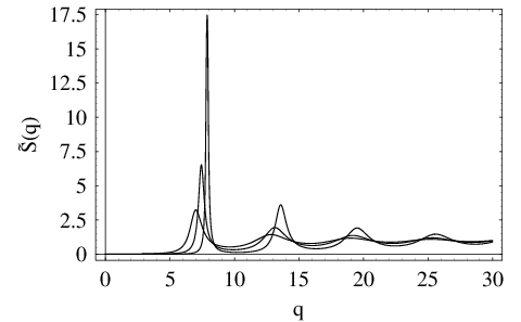
Refer to caption
Refer to caption
Refer to caption
Figure 1: The static structure factor as determined using the Percus-Yevick Hard Sphere Approximation for (a) η=0.1\eta=0.1, 0.20.2, 0.30.3, and 0.40.4, (b) η=0.5\eta=0.5, 0.60.6 and 0.70.7, and (c) η=0.8\eta=0.8. Larger first structure peak height corresponds to larger η\eta within each plot.

The numerical solution of Eq.(216) for V~​(q)\tilde{V}(q) is obtained as follows. First, rewrite Eq.(216) in the form

V~=S~−1−1+M⁡(V~).\displaystyle\tilde{V}=\tilde{S}^{-1}-1+M(\tilde{V}). (220)

Next, define

V0=S~−1−1\displaystyle V_{0}=\tilde{S}^{-1}-1 (221)

and rewrite

V~=V0+Q⁡(V~),\displaystyle\tilde{V}=V_{0}+Q(\tilde{V}), (222)

where

Q⁡(V~)=M⁡[V0+Q⁡(V~)]≡I⁡(Q).\displaystyle Q(\tilde{V})=M[V_{0}+Q(\tilde{V})]\equiv I(Q). (223)

We seek an iterated solution. To this end, we write

α​Qℓ+1+(1−α)​Qℓ=I⁡(Qℓ)\displaystyle\alpha Q_{\ell+1}+(1-\alpha)Q_{\ell}=I(Q_{\ell}) (224)

with the number α\alpha chosen appropriately. This equation can be rewritten as a functional recursion relation,

Qℓ+1=Qℓ+1α​[I⁡(Qℓ)−Qℓ].\displaystyle Q_{\ell+1}=Q_{\ell}+\frac{1}{\alpha}[I(Q_{\ell})-Q_{\ell}]. (225)

At a fixed point we have a solution to the original problem. By trial and error we find that a reasonable choice for α\alpha is α=100.\alpha=100. Then beginning with Q0=0Q_{0}=0 we monitor

Δℓ=4​∑q(V~ℓ+1−V~ℓ)2∑q(V~ℓ+1+V~ℓ)2.\displaystyle\Delta_{\ell}=4\frac{\sum_{q}(\tilde{V}_{\ell+1}-\tilde{V}_{\ell})^{2}}{\sum_{q}(\tilde{V}_{\ell+1}+\tilde{V}_{\ell})^{2}}. (226)

Over the entire range of η\eta studied, we find that Δℓ\Delta_{\ell} is driven to small values (10−610^{-6}-10−810^{-8}) with a minimum controlled by the range of wavenumber included in the calculation. One obtains good accuracy if one chooses qm​a​x=80q_{max}=80.

In Fig.2 we give the results for the effective potential for a sequence of densities. Also shown is V0V_{0}. A key quantity is V~​S~\tilde{V}\tilde{S}. It is plotted in Fig. 3 where we also plot V0​S~V_{0}\tilde{S}. Clearly the two quantities are close and do not change dramatically in going from first to second order. The biggest shift is for small wavenumbers. That M⁡(q)M(q) has a maximum for small qq is understood by assuming that V~​(k)​S~​(k)\tilde{V}(k)\tilde{S}(k) is sharply peaked for k=k0k=k_{0}. Therefore V~​(k)​S~​(k)​V~​(k+q)​S~​(k+q)\tilde{V}(k)\tilde{S}(k)\tilde{V}(k+q)\tilde{S}(k+q) is small except when k≈|q+k|≈k0k\approx|q+k|\approx k_{0} which is true for small qq.

Refer to caption
Refer to caption
Refer to caption
Refer to caption
Refer to caption
Refer to caption
Refer to caption
Refer to caption
Figure 2: The zeroth order potential V~0​(q)\tilde{V}_{0}(q) and the numerical solution for the full potential V~​(q)\tilde{V}(q) from (a) η=0.1\eta=0.1 to (h) η=0.8\eta=0.8 in increments of 0.1.
Refer to caption
Refer to caption
Refer to caption
Refer to caption
Refer to caption
Refer to caption
Refer to caption
Refer to caption
Figure 3: The potential times the static structure factor for both V~0​(q)\tilde{V}_{0}(q) and V~​(q)\tilde{V}(q) from (a) η=0.1\eta=0.1 to (h) η=0.8\eta=0.8 in increments of 0.1.

XII ENE Transition

As we increase the density, (or lower the temperature), our model system slows down. It is possible that there is a density above which the density-density correlation does not decay to zero for long times. In the nonergodic phase

limt→∞Gρ​ρ​(q,t)=F⁡(q)>0.\displaystyle\lim_{t\rightarrow\infty}G_{\rho\rho}(q,t)=F(q)>0.

In terms of the time Fourier transform,

Gρ​ρ​(q,ω)=F⁡(q)​2​π​δ​(ω)+gρ​ρ​(q,ω),\displaystyle G_{\rho\rho}(q,\omega)=F(q)2\pi\delta(\omega)+g_{\rho\rho}(q,\omega), (227)

where gρ​ρg_{\rho\rho} is the regular contribution. In the nonergodic phase, assuming the FDT still holds, one has for the response function

Gρ​B​(q,ω=0)=∫−∞∞Gρ​B​(q,t)\displaystyle G_{\rho B}(q,\omega=0)=\int_{-\infty}^{\infty}G_{\rho B}(q,t)
=β​∫−∞∞θ⁡(t)​∂∂t​Gρ​ρ​(q,t)\displaystyle=\beta\int_{-\infty}^{\infty}\theta(t)\frac{\partial}{\partial t}G_{\rho\rho}(q,t)
=β​∫0∞∂∂t​Gρ​ρ​(q,t)=β⁡[F⁡(q)−S⁡(q)]\displaystyle=\beta\int_{0}^{\infty}\frac{\partial}{\partial t}G_{\rho\rho}(q,t)=\beta[F(q)-S(q)] (228)

while

GB​ρ​(q,ω=0)=∫−∞∞GB​ρ​(q,t)\displaystyle G_{B\rho}(q,\omega=0)=\int_{-\infty}^{\infty}G_{B\rho}(q,t)
=β​∫−∞∞θ⁡(−t)​(−1)​∂∂t​Gρ​ρ​(q,t)\displaystyle=\beta\int_{-\infty}^{\infty}\theta(-t)(-1)\frac{\partial}{\partial t}G_{\rho\rho}(q,t)
=β​∫−∞0(−1)​∂∂t​Gρ​ρ​(q,t)=−β​S​(q).\displaystyle=\beta\int_{-\infty}^{0}(-1)\frac{\partial}{\partial t}G_{\rho\rho}(q,t)=-\beta S(q). (229)

There are several equivalent ways of determining the nonergodicity parameter FF as a function of density and temperature. One approach developed in the time-domain results from pursuing the memory-function equation, Eq.(83). This will be explored elsewhere. Here we give a more direct complementary analysis in frequency space.

Using one of the Dyson equations we have

Gρ​ρ​(q,ω)=−Gρ​B​(q,ω)​ΓB​B​(q,ω)​GB​ρ​(q,ω).\displaystyle G_{\rho\rho}(q,\omega)=-G_{\rho B}(q,\omega)\Gamma_{BB}(q,\omega)G_{B\rho}(q,\omega). (230)

For an ENE transition we associate a zero-frequency delta-function in ΓB​B\Gamma_{BB}

ΓB​B​(q,ω)=−2​π​δ​(ω)​Γ¯​(q)+regular part.\displaystyle\Gamma_{BB}(q,\omega)=-2\pi\delta(\omega)\bar{\Gamma}(q)+\textrm{regular part}. (231)

Then, using Eqs.(227) and (231) in Eq. (230), we find

F⁡(q)=β2​Γ¯​(q)​[S⁡(q)−F⁡(q)]​S​(q).\displaystyle F(q)=\beta^{2}\bar{\Gamma}(q)[S(q)-F(q)]S(q). (232)

Equation (232) can be rewritten as

F⁡(q)S⁡(q)−F⁡(q)=S⁡(q)​β2​Γ¯​(q).\displaystyle\frac{F(q)}{S(q)-F(q)}=S(q)\beta^{2}\bar{\Gamma}(q).

We need to extract the lowest order approximation for Γ¯\bar{\Gamma}. We have from our previous work that

β2​ΓB​B(2)​(1)=I​m​𝒪​[R−​(1+i​E1)2]\displaystyle\beta^{2}\Gamma_{BB}^{(2)}(1)=Im{\cal O}[R_{-}(1+iE_{1})^{2}]
=−ρ0−4∫d​ω¯32​πd​ω¯42​πdd​k¯3(2​π)ddd​k¯4(2​π)dδ(q+k¯3+k¯4)G¯ρ​ρ(k¯3,ω¯3)G¯ρ​ρ(k¯4,ω¯4)\displaystyle=-\rho_{0}^{-4}\int\frac{d\bar{\omega}_{3}}{2\pi}\frac{d\bar{\omega}_{4}}{2\pi}\frac{d^{d}\bar{k}_{3}}{(2\pi)^{d}}\frac{d^{d}\bar{k}_{4}}{(2\pi)^{d}}\delta(q+\bar{k}_{3}+\bar{k}_{4})\bar{G}_{\rho\rho}(\bar{k}_{3},\bar{\omega}_{3})\bar{G}_{\rho\rho}(\bar{k}_{4},\bar{\omega}_{4})
×I​m​𝒪​[R−​(1+i​E1)2].\displaystyle\times Im{\cal O}[R_{-}(1+iE_{1})^{2}].

In the nonergodic phase we have the δ\delta-function contribution

G¯ρ​ρ​(k¯3,ω¯3)=−ρ0​β​V​(k¯3)​F​(k¯3)​2​π​δ​(ω¯3)\displaystyle\bar{G}_{\rho\rho}(\bar{k}_{3},\bar{\omega}_{3})=-\rho_{0}\beta V(\bar{k}_{3})F(\bar{k}_{3})2\pi\delta(\bar{\omega}_{3}) (233)

and we find immediately that we can set E1=0E_{1}=0, and

I​m​R−=π​δ​(ω1+ω3+ω4)=π​δ​(ω1).\displaystyle ImR_{-}=\pi\delta(\omega_{1}+\omega_{3}+\omega_{4})=\pi\delta(\omega_{1}). (234)

Comparing with Eq.(231),

β2​Γ¯B​(q)=12​ρ04​∫dd​k(2​π)d​ρ0​β​V​(k)​F​(k)​ρ0​β​V​(q+k)​F​(q+k).\displaystyle\beta^{2}\bar{\Gamma}_{B}(q)=\frac{1}{2\rho_{0}^{4}}\int\frac{d^{d}k}{(2\pi)^{d}}\rho_{0}\beta V(k)F(k)\rho_{0}\beta V(q+k)F(q+k).

It is useful to write

F⁡(q)=S⁡(q)​f​(q)\displaystyle F(q)=S(q)f(q) (235)

and it is f⁡(q)f(q) that is conventionally called the ergodicity parameter.

Using the same set of dimensionless variables as in the static calculations, the nonergodicity equation can be written in the conventional form

f⁡(q)1−f⁡(q)=w⁡(q),\displaystyle\frac{f(q)}{1-f(q)}=w(q), (236)

where

w⁡(q)=π12​η​S~​(q)​∫dd​k(2​π)d​V~​(k)​f​(k)​S~​(k)​V~​(q+k)​f​(k+q)​S~​(q+k).\displaystyle w(q)=\frac{\pi}{12\eta}\tilde{S}(q)\int\frac{d^{d}k}{(2\pi)^{d}}\tilde{V}(k)f(k)\tilde{S}(k)\tilde{V}(q+k)f(k+q)\tilde{S}(q+k). (237)

Before solving Eq.(236) numerically, it is useful to obtain an approximate analytical solution. Notice that the combination V~​(k)​S~​(k)\tilde{V}(k)\tilde{S}(k) (see Fig. 3) is sharply peaked at the structure factor maximum. Then, to a reasonable approximation, we can replace f⁡(k)f(k) with its value at the maximum such that

w⁡(q)=f2​(q0)​S~​(q)​M​(q)\displaystyle w(q)=f^{2}(q_{0})\tilde{S}(q)M(q) (238)

with M⁡(q)M(q) the same quantity that appears in the static calculation. Putting this result in the nonergodicity equation we obtain

f⁡(q)1−f⁡(q)=f2​(q0)​w~​(q),\displaystyle\frac{f(q)}{1-f(q)}=f^{2}(q_{0})\tilde{w}(q), (239)

where

w~​(q)=S~​(q)​M~​(q)\displaystyle\tilde{w}(q)=\tilde{S}(q)\tilde{M}(q) (240)

is known from our static structural calculations. We now have a closed algebraic equation for f⁡(q0)f(q_{0}) if we set q=q0q=q_{0} in Eq.(239) with f0=f⁡(q0)f_{0}=f(q_{0}) and w0=w~​(q0)w_{0}=\tilde{w}(q_{0}):

f01−f0=f02​w0.\displaystyle\frac{f_{0}}{1-f_{0}}=f_{0}^{2}w_{0}. (241)

Discarding the ergodic solution f0=0f_{0}=0, we have a quadratic equation to solve given by

w0​f02−w0​f0+1=0\displaystyle w_{0}f_{0}^{2}-w_{0}f_{0}+1=0 (242)

with the solution

f0=12​(1+1−4/w0).\displaystyle f_{0}=\frac{1}{2}\left(1+\sqrt{1-4/w_{0}}\right). (243)

Note that there is no transition for w0<4w_{0}<4. For w0>4w_{0}>4, we obtain the full wave number dependence by putting f0f_{0} back into

f⁡(q)=w~​f021+w~​f02.\displaystyle f(q)=\frac{\tilde{w}f_{0}^{2}}{1+\tilde{w}f_{0}^{2}}. (244)

It is easy to compute the w0w_{0} numerically using the Percus Yevick (PY) structure factor. In Fig. 4 we plot w0w_{0} versus η\eta. We find that the ENE transition density, when w0=4w_{0}=4, is η∗=0.53\eta^{*}=0.53. The associated f⁡(q)f(q) is shown in Fig. 5 for several densities in the nonergodic phase.

Refer to caption
Refer to caption
Figure 4: Values of w0w_{0} versus η\eta. Note that the line crosses w0=4w_{0}=4 (and therefore enters the nonergodic regime) near η=0.525\eta=0.525. (The solid line is to guide the eye only.)
Refer to caption
Refer to caption
Refer to caption
Refer to caption
Refer to caption
Refer to caption
Figure 5: Using the analytic approximation for f(q) given by Eq. (244), we plot the approximate form of the nonergodicity parameter for (a) η=0.53\eta=0.53 (just above the analytic transition), (b) η=0.55\eta=0.55, (c) η=0.60\eta=0.60, (d) η=0.65\eta=0.65, (e) η=0.70\eta=0.70 and (f) η=0.75\eta=0.75.

Returning to the full problem, Eq.(236) can be rewritten in the form

f⁡(q)=w⁡(q)1+w⁡(q).\displaystyle f(q)=\frac{w(q)}{1+w(q)}. (245)

The solution of this equation is available via direct iteration. If we use an initial trial value of f0​(q)=1/2f_{0}(q)=1/2 in Eq.(237), we generate an initial trial value w0=0.25​S~​(q)​M​(q)w_{0}=0.25\tilde{S}(q)M(q) to obtain

f1​(q)=w0/(1+w0).\displaystyle f_{1}(q)=w_{0}/(1+w_{0}). (246)

We continue iterating via

fℓ+1​(q)=wℓ/(1+wℓ)\displaystyle f_{\ell+1}(q)=w_{\ell}/(1+w_{\ell}) (247)

and find that

limℓ→∞(fℓ+1−fℓ)=0.\displaystyle\lim_{\ell\rightarrow\infty}(f_{\ell+1}-f_{\ell})=0. (248)

For pure hard-sphere systems in three dimensions we find an ergodic-nonergodic transition at η∗=0.76\eta^{*}=0.76. Clearly this density is physically unattainable. It is interesting to solve Eq.(245) using the first order result V~=S~−1−1\tilde{V}=\tilde{S}^{-1}-1 rather than the second order result. Despite the fact that there is small change in the effective potential in going from first to second order one finds a substantial change in the critical density from 0.760.76 to 0.600.60. Thus, we see that η∗\eta^{*} is a sensitive quantity.

In Fig. 6 we plot f⁡(q)f(q) for hard spheres for a set of η>η∗\eta>\eta^{*}. We find a lot of structure in f⁡(q)f(q). Comparing the approximate f⁡(q)f(q) given in Fig. 5 with the full numerical solution we see good agreement despite very different transition densities.
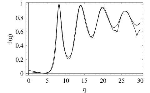
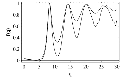
Refer to caption
Refer to caption
Figure 6: Numerically, we find a transition at η=0.763\eta=0.763. We plot the numerical solution and the analytic solution for (a) η=0.763\eta=0.763 and (b) η=0.8\eta=0.8. The more ragged and slightly lower line in each plot is the analytic approximation.

XIII Conclusions

We established here that the theory of time-dependent fluctuations in equilibrium can be organized around the fluctuation-dissipation theorem. Using the FDT one can relate the two-point response function to the two-point correlation function. In turn this gives a linear-relation between self-energy components. We show more specifically the nontrivial result that the collective parts of the self-energies at second order satisfy a FDT. We find the second order self-energies as functionals of the physical density-density correlation functions. The role of the three-point vertex functions are crucial in this analysis.

Using the FDT the static structure is separated from the dynamical information and gives one a self-consistent expression for the static structure factor in terms of the potential. This expression can be recovered from a strictly static analysis. We show how the problem can be turned around and posed as in MCT. The structure factor is assumed to be given and we solve for the effective potential V~\tilde{V} that produces the known structure factor. At first order, the effective potential is proportional to the static direct correlation function. At second order, V~\tilde{V} is similar to the first order result except at small wavenumbers.

We also show that the theory is compatible with an ENE transition at second order. The critical density is sensitive to the details of the calculation. Using the Percus-Yevick approximation for hard spheres we find an ENE transition at the physically inaccessible density η∗=0.76\eta^{*}=0.76.

In a future work we will explore the role of the single-particle dynamics which occur in this theory. The treatment of these degrees of freedom gives one information about the equation of state, ⟨ρ⟩=ρ¯​(ρ0,T)\langle\rho\rangle=\bar{\rho}(\rho_{0},T). The single-particle degrees of freedom contribute a second order contribution to the self-energies which depends on the full density-density correlation function.

Our focus here, because of its simplicity, has been on Smoluchowski dynamics, but as will be discussed elsewhere, the method developed here can be applied to Newtonian dynamics and Fokker-Planck dynamics as well as a broader class of models.

The approach presented here allows for a systematic method for analyzing corrections to this second order result including determination of higher order correlation functions. We plan to analyze the third order contribution to the collective self-energy soon.

We guess that the theory presented here can be organized to give a theory of freezing. One can then do simultaneous free energy comparisons between the nonergodic state and the crystalline solid state.

Acknowledgements.
I thank the Physics Department and the Joint Theory Institute at the University of Chicago for support. A special thanks is due to M. Zannetti for showing that Gρ​BG_{\rho B} satisfies a simple linear fluctuation-dissipation theorem and for other comments on this work. I thank David McCowan for help with the figures and comments and I thank Paul Sprydis and S. Das for their comments on this work.

References

  • [1] G. F. Mazenko, Phys. Rev. E 81, 061102 (2010). (Referred throughout as FTSPD.)
  • [2] A. Andreanov, G. Biroli and A. Lefevre, ”Dynamical Field Theories for glass forming liquids,” J. Stat. Mech.: Theory Exp. PO7008 (2006).
  • [3] S. Das, Rev. Mod. Phys. 76, 785 (2004).
  • [4] A. Crisanti, Nuc. Phys. B796, 425 (2008).
  • [5] W. Goetze in Liquids, Freezing and Glass Transition, edited by Hansen J. P., Levesque D. and Zinn-Justin J. (North-Holland, Amsterdam) 1991; and S. Das, Rev. Mod. Phys. 76, 785 (2004).
  • [6] There is an exact solution to the Percus-Yevick approximation for hard spheres. See the discussion in Chapter 4 in J.-P. Hansen and I. R. McDonald, Theory of Simple  Liquids, Third Ed., (Academic, New York 2006); N. W. Ashcroft and J. Lekner, Phys. Rev. 145, 83 (1966).
  • [7] A. Crisanti (private communication).
  • [8] The F12F_{12} model and stretching are discussed in detail by W. Goetze, in Liquids, Freezing and Glass Transition, edited by Hansen J. P., Levesque D. and Zinn-Justin J. (North-Holland, Amsterdam) 1991.
  • [9] P. N. Pusey, J. Phys. Condens. Matter 20, 434202 (2008).
  • [10] The classical operator formalism for Newtonian dynamics was introduced by J. von Neumann, Proc. Natl. Acad. Sci. U.S.A. 18, 70 (1932); H. Koopman and J. von Neumann, ibid 18, 255 (1932).
  • [11] The history of Smoluchowski dynamics is discussed in FTSPD.
  • [12] A brief discussion of the storied history of Brownian motion is given in Refs. 2 and 20 in FTSPD. We will refer to the noninteracting limit of Smoluchowski dynamics as the Brownian gas.
  • [13] D. S. Dean, J. Phys. A29, L613, (1996).
  • [14] K. Kawasaki and S. Miyazima, Z. Phys. B: Cond. Matter 103, 423 (1997).
  • [15] MSR actions are discussed in Appendix A in FTSPD.
  • [16] B. Kim and K. Kawasaki, ”A FDR-Preserving Field Theory for Interacting Brownian Particles: One-Loop Theory and MCT,” AIP Conf. Proc. 982 (Complex Systems: 5th International Workshop on Complex Systems,” Sendai (Japan), Sept. 22-28, 2007.), 223 (2008).
  • [17] R. Velenich, C. Chamon, L. Cugliandolo, and D. Kreimer, J. Phys. A41, 235002 (2008).
  • [18] See the discussion in FTSPD.
  • [19] The static Ornstein-Zernike relation that connects the radial distribution function to the direct correlation function.
  • [20] In different contexts the kinetic kernels have different names. In the field theory context the kernels are typically called self-energies, in the kinetic theory case, where the analysis is in terms of retarded quantities, the kernel is called a memory function, and in the general case it can be called a dynamic direct correlation function.
  • [21] Note that b1b_{1} depends on the nn tit_{i} while the operator depends only on t1t_{1}.
  • [22] G. F. Mazenko, D. D. McCowan and P. Spyridis, in preparation.
  • [23] An advantage of working in equilibrium is that we can take the initial time to minus infinity. We called this the field-theory protocol in FTSPD.