QCD-Thermodynamics using 5-dim Gravity
Abstract
We calculate the critical temperature and free energy of the gluon plasma using the dilaton potential [1] in the gravity theory of AdS/QCD. The finite temperature observables are calculated in two ways: first, from the Page-Hawking computation of the free energy, and secondly using the Bekenstein-Hawking proportionality of the entropy with the area of the horizon. Renormalization is well defined, because the theory has asymptotic freedom. We further investigate the change of the critical temperature with the number of flavours induced by the change of the running coupling constant in the quenched theory. The finite temperature behaviour of the speed of sound, spatial string tension and vacuum expectation value of the Polyakov loop follow from the corresponding string theory in .
1 INTRODUCTION
In the bottom-up approach of AdS/QCD important properties of pure glue QCD are encoded in a phenomenological gravity theory through the introduction of a dilaton potential. The fifth dimension plays the role of an inverse energy scale, which necessitates that the dilaton is not constant, but runs with this scale. In a previous paper [1] we have fixed the ultraviolet behaviour of the potential to the two loop beta function of QCD and parametrized the infrared part in such a way that the heavy potential is reproduced. In five dimensions the string connecting the and hangs into the bulk fifth dimension and thereby is sensitive to the geometry of the five dimensional space. An obvious next step is to consider properties of QCD in other simple environment where the geometry of the five dimensional space changes in a controlled manner.
Finite temperature properties of QCD are on top of the list, since they mostly concern spatially homogeneous systems, where the equations of motion are still simple to solve. There has been quite some understanding of the deconfinement transition in 4-dimensions on the basis of strings in strong coupling lattice QCD. It comes from a roughening of the strings due the entropic enhancement of configurations with long wiggly strings. The high temperature phase, however, is not understood in a picture where the underlying degrees of freedom are strings at low temperature. Indeed the old Hagedorn picture is limited to temperatures below the phase transition. Above the critical temperature spatio-temporal Wilson loops are no longer suppressed due to their area, the string tension goes to zero and therefore strings have seized to live in the plasma. There is a remnant of the low temperature theory in the behaviour of purely spatial Wilson loops, but this effect is not very strong at high temperatures. In Refs. [2] an analysis of the contribution due to these spatial surfaces has been made in 4- dimensions. There have been various attempts to analytically continue effective 4-dimensional string theories to the deconfinement phase, see e.g. Refs. [3, 4, 5], however without any phenomenological application so far.
The duality of string theory with 5-dimensional gravity can help. In conformal the metric is well known. It has a horizon in the bulk space at where , the inverse of temperature, and is the radius of the AdS-space. Conformal solutions for entropy scale like , since the 3-dimensional area of the horizon is given as . Promising solutions of this conformal theory have been proposed to the problem of viscosity [6] with a small constant value for . Top to bottom approaches based on the conformal SYM with fermions have been investigating the chiral phase transition and problems at finite density [7, 8].
Indeed there may be a window with the plasma not close to the phase transition and not yet perturbative, where this conformal theory mimics truthfully reality. With solutions at at hand [1, 9] which break conformal symmetry and give confinement, it is challenging to investigate the sector of the theory for all temperatures. Important progress has been made in this direction by two groups [10, 11].
In this paper we follow this general approach, and investigate the equation of state with two different methods. On the one hand we use the Hawking-Page formalism [12] to derive the renormalized free energy from the action. On the other hand we directly calculate the entropy from the Bekenstein-Hawking formula [13]. These two approaches are assumed to give identical results as long as the black hole is treated entirely classical. Renormalization is well defined, because the theory has asymptotic freedom. We further investigate the change of the critical temperature with the number of flavours induced by the change of the running coupling constant. In a renormalization group framework interesting behaviour of has been demonstrated recently [14]. Finally using the string theory we can investigate the finite temperature behaviour of several thermodynamic quantities, like the speed of sound, spatial string tension and vacuum expectation value of the Polyakov loop. Comparison with lattice data is made.
The outline of the paper is as follows: In Section 2 we give an overview of the 5-d gravity action and specify the dilaton potential which is used. In Section 3 we will reproduce the zero temperature results focussing on the behaviour of the metric and the coupling near the boundary . Section 4 gives the finite temperature calculation emphasizing the similarities and differences of the two solutions at the boundary. Section 5 is devoted to deduce the thermodynamics of the plasma using the Page-Hawking approach. In Section 6 we discuss the Bekenstein-Hawking approach to compute the free energy, and compare with the method of previous section. We also discuss the consequences of the flavour dependence of the running coupling. In Section 7 we compute the thermal behaviour of speed of sound, spatial string tension and vacuum expectation value of the Polyakov loop, and its comparison with available lattice data. Finally, Section 8 gives a final discussion and our conclusions. In Appendix A we discuss in details the procedure to solve numerically the Einstein equations at finite temperature. In Appendix B we show technical details for the analytical computation of thermodynamic quantities in the ultraviolet regime.
2 5-d gravity action
In the large limit, we assume a five dimensional gravity-dilaton model, with the action
| (1) |
The last term is the Gibbons-Hawking term, where the integration is evaluated at the boundary of the five dimensional space given by . The induced metric on the surface is denoted by . An infinitesimal distance to the boundary is used to regularize our expressions. Later we will take the limit . The metric is taken in the Einstein frame, and the extrinsic curvature or second fundamental form of the boundary, , is evaluated with the help of the normal at the boundary :
| (2) | |||||
| (3) |
In Ref. [1] we extrapolated the -function of QCD to the infrared with a parametrization which was consistent with asymptotic freedom and the heavy potential at zero temperature. This parametrization takes the form
| (4) |
where
| (5) |
is the running coupling. With this -function we could obtain the dilaton potential in AdS/QCD as a function of the running coupling constant:
| (6) | |||||
where is the exponential integral function. For the potential is strictly determined by the perturbative -function,
| (7) | |||||
| (8) | |||||
| (9) |
The parameters and are universal, i.e. they are regularization scheme independent. For the -function behaves linearly, , and the potential is characterized by the non-perturbative constants and . The parametrized coefficient has the form
| (10) |
From the heavy potential at zero temperature one gets the optimum values [1]
| (11) |
The potential itself approaches the conformal limit for . Based on this action we will investigate the thermodynamics of QCD.
Our parametrization given by Eq. (4) is simple and more intuitive than that of Ref. [15]. It allows for analytical computations in many cases, e.g. we can derive analytically the dilaton potential Eq. (6) from the -funtion Eq. (4). The dilaton potential of Ref. [15] is fine tuned and the role played by their parameters are not so obvious. We plot in Fig. 1 the dilaton potential of Eq. (6) which we use in this work, and compare it with the one proposed in Ref. [15] which we call . We use in both cases the same value of given by Eq. (11). is of the order of in the regime of our interest, , in contrast to the value given by our potential . Both potentials share the same ultraviolet behaviour, but they differ in the infrared. Since the scheme dependent coefficient in Ref. [15] is very much larger than ours, the running of the coupling of Ref. [15] deviates already for extremely small values from the regime dictated by the leading coefficients and and then it depends entirely on the “infrared” parametrisation in the regime of our interest. In the scheme of Ref. [15] the values of sampling the dilaton potential are much smaller over the whole range of temperatures. At e.g. or more than 100-times smaller than the usual running coupling in scheme . This explains the large difference between the dilaton potentials when they are plotted as a function of the same . Unfortunately no mapping between and in our - scheme is known. A further discussion will be presented in Section 6.

3 Thermal gas solution of the Einstein Equations
The equations of motion corresponding to the five dimensional gravity-dilaton action, Eq. (1), are given by
| (12) |
with
| (13) | |||||
| (14) |
The left hand side of Eq. (12) is the Einstein tensor while the right hand side is the energy momentum tensor . The Thermal Gas solution preserves spatial rotational invariance and it has a metric similar to the zero temperature solution in Euclidean space:
| (15) | |||||
| (16) |
where is the bulk coordinate in the fifth dimension, and the imaginary time coordinate is periodic with period , the inverse of temperature. This solution exists at all temperatures. Under the assumption that the energy scale is proportional to , i.e. , the -function writes
| (17) |
There will be a second solution at finite temperature, the Black Hole solution, with a horizon in the bulk coordinate which characterizes the gluon plasma, and which we will discuss in the next section. After computing the Einstein tensor and the energy momentum tensor in terms of and its derivatives, one ends up with three equations which determine the thermal gas solution:
| (18) | |||
| (19) | |||
| (20) |
In the following text stands for derivative with respect to the coordinate. In order to reduce the equations of motion to first order equations, we have introduced the superpotential defined as
| (21) |
This definition agrees with the one given in Ref. [1]. The functions , and characterizing this solution have the index . We replace the variable , dilaton potential, by the running coupling .
The system Eqs. (18)-(20) has been solved numerically in Ref. [1] by considering the bulk coordinate at which is mapped to the energy by the metric factor and the arbitrary scale . The choice of scale size has only historical reasons, and in principle the mapping of the energy coordinate to the z-coordinate has an arbitrary constant. The resulting parametrization of the -function and dilaton potential would then also change. We use this scale, because we did not want to recalculate the fit to the running coupling and the string tension with another energy scale. The value of the running coupling at follows from the experimental PDG data of the running coupling, c.f. Ref. [16], and it is . The value of comes from the Einstein equations which allow an explicit solution of the superpotential in terms of and ,
| (22) | |||||
| (23) | |||||
| (24) |
We have solved the above equations and verified that they give the same solutions as obtained in the previous paper on zero temperature Ref. [1]. Note the finite temperature does not enter in the gravity equations dependent on . The thermal gas is solely defined by the periodicity in . The initial conditions fix the running of the coupling in the bulk and its scale which we compute from the numerical solution. Given the perturbative -function, which is parametrized for higher orders in Ref. [1]
| (25) |
the running coupling has the form:
| (26) | |||||
with
| (27) |
and the definition
| (28) |
The ultraviolet expansion of follows from Eqs. (19) and (20), using for the expansion given by Eq. (26). Then reads
| (29) | |||||
In order to compute accurately the value of , one can consider as a function of and expand it around the point where the initial conditions were given. The expansion writes
| (30) | |||||
For a fit of the numerical solutions for and to the form given in Eqs. (26) and (30) respectively, yields in both cases which is a factor two larger than . The parameter is an integration constant which appears in the Gell-Mann-Low integral [17]. Note that a particular choice of fixes the definition of . We have chosen in this computation .
4 Black hole solution of the Einstein Equations
The gravitational equations have two different types of solutions for the metric. Besides the thermal gas solution which we discussed in the previous section, there is also a solution which has a horizon localized in the bulk coordinate at similar to the situation in 4-dim gravity. The phenomenology of the gluon plasma arises from the competition of the free energies computed in both metrics. When the free energy of the black hole solution has a lower value than the thermal gas solution, the phase transition to the quark gluon plasma takes place [12].
Now we will discuss the equations of motion at finite temperature using the black hole metric. The procedure is similar as discussed above for the zero temperature case, but a new equation appears due to the black hole factor . The black hole metric in Einstein frame has the form:
| (31) | |||||
| (32) |
where
| (33) | |||||
| (34) |
Near the horizon the metric is given by
| (35) |
We define a new variable . In terms of we obtain
| (36) |
The - portion of the metric defines a two-plane in polar coordinates with serving as the angular coordinate. To avoid a conical singularity at we must require that has a period of . In Matsubara (imaginary-time) formalism the period is equal to inverse temperature . Thus, the temperature of a black hole solution is given by [18, 19]
| (37) |
The Einstein tensor and energy momentum tensor have different components in , and spatial directions, and can be expressed in terms of , , dilaton field , dilaton potential and its derivatives. One ends up with the four equations relevant at
| (38) | |||
| (39) | |||
| (40) | |||
| (41) |
where we have introduced the superpotential at finite temperature which is defined in analogy with Eq. (21),
| (42) |
Note that the system of Eqs. (38)-(41) reduces to the zero temperature formulas Eqs. (18)-(20) when . Our prescription is to use the same dilaton potential at zero and finite temperature. Note, however, that is affected by the temperature dependence of , i.e. . In order to solve the system of equations (38)-(41) one should specify five initial conditions, as one has to handle three differential equations of first order, Eqs. (38)-(40), and one differential equation Eq. (41) of second order. The Eq. (41) for the black hole function can be solved analytically in terms of . Since our set up includes asymptotic freedom, is different from the conformal solution . Also the black hole factor deviates from the simple form of the conformal solution . Using Eq. (39) one gets
| (43) |
where the first integration constant has been chosen such that . The second integration constant is fixed to unity by the requirement . From Eq. (37) and the definition of given by Eq. (43), one derives easily the useful relation
| (44) |
The technical procedure to solve numerically the Einstein equations is explained in details in Appendix A. We show in Figs. 2, 3, 4 and 5 the solutions for , , and obtained at the temperature MeV and compare them in the same figures with the zero temperature solutions as computed in Sec. 3. Note that the and solutions agree in the ultraviolet, i.e. , but differ in the infrared due to the thermal fluctuations introduced by the black hole horizon at .


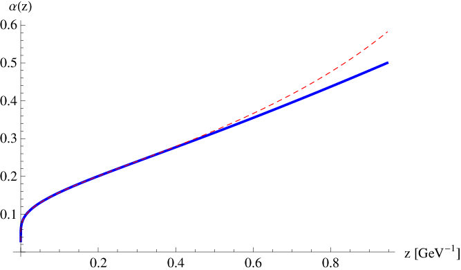
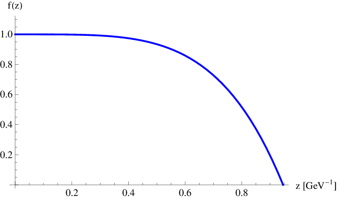
As we will explain in Sec. 5, we use to extract the trace anomaly. The finite temperature solution differs from the zero temperature one at order . Care has to be taken to keep track of leading logarithmic effects which are not usually considered, c.f. Ref. [10], but are important if one wants to calculate the gluon condensate . The difference between zero and finite temperature solutions is mainly given by the gluon condensate or the trace anomaly which equals up to normalization factors,
| (45) |
The subscripts and stand for the thermal and vacuum values of respectively. The expressions relating zero and finite temperature quantities read up to
| (46) | |||||
| (47) | |||||
| (48) | |||||
| (49) |
where
| (50) |
being given by (c.f. Appendix B)
| (51) |
Higher orders in and in Eqs. (46)-(49) are indicated by dots.
To arrive at Eqs. (47)-(49) we have assumed for an expansion of the form given by Eq. (46), and used the equations of motion Eqs. (39)-(40). Note that on the r.h.s. of these expressions, inside the brackets, one can substitute by and the expressions remain valid at this order, as the difference between both quantities, and , is , c.f. Eq. (47). To get the values of the coefficients and , one has to substitute the expansions for , and into the first equation of motion, Eq. (38), and use the assumption that the dilaton potential at finite temperature as a function of the dilaton field has the same functional form as the one at zero temperature, i.e. . Then one gets
| (52) | |||||
| (53) |
where is defined in Eq. (43). Note that the expression of in Eq. (53) means that in the expansion of the quantities in powers of , Eqs. (46)-(49), there are contributions not only of the gluon condensate , but also of . The leading contribution involving is times the corresponding quantity at zero temperature ( in the case of ).
The contribution of in Eqs. (46)-(49) is visible in Figs. 2-4, and all these figures consistently show that is positive. Note that in our set-up the correction arising from the NLO and NNLO coeficients of the -term are not small in the infrared, since at . Therefore we have to resort to a UV-analysis to determine the gluon condensate G from the computation of .
5 Free energy from the Einstein-Hilbert action
To get the thermodynamics of the five dimensional gravity-dilaton model of Eq. (1) one computes the free energy at fixed temperature by introducing a lower cut off in the integral over the on shell action:
| (54) |
Regularization is needed due to ultraviolet divergences near the holographic boundary . The procedure to compute the regularized action with the black hole solution is explained in details in Ref. [10]. The free energy is computed as the difference between the free energy of the black hole solution and that of the thermal gas solution, so by definition the later has zero free energy. The result for the free energy is [10]
| (55) |
From one can compute the pressure and the rest of thermodynamic quantities by applying the thermodynamic relations. The values of and in the ultraviolet are given by (c.f. Appendix B)
| (56) | |||||
| (57) |
Inserting Eqs. (56) and (57) into Eq. (55) one gets the UV assymptotic expansion of the free energy which will be discussed later. To deal with Eq. (55) at temperatures near one has to compute the temperature dependence of and numerically. Using Eq. (44) one can calculate from the numerical result of . On the other hand the temperature dependence of can be computed by comparing the thermal gas and black hole solutions in the ultraviolet, using Eqs. (46)-(49). In the UV we perform a fit of the difference , and compute the coefficient for different temperatures. Note that it is much more efficient to use instead of , as the latter diverges in the UV making it more difficult to get reliable results for . In this paper we have analyzed carefully the expansion of the term in , Eq. (47), which gives the trace anomaly in the plasma. Higher order terms in affect appreciably the fit of , and it is indispensable to consider at least the order to get good agreement of the thermodynamic quantities with the numerical results from the Bekenstein-Hawking entropy formula as computed in Sec. 6. Up to it reads
| (58) |
where and are given by Eqs. (52) and (50) respectively. In Fig. 6 we show the numerical and analytical results of for small z. Note that this quantity is not flat in this region, and a rough fit with a constant term (constant in ) leads in general to an overestimation of the value of , and then also on the value of , c.f. Eq. (55). This induces an appreciable error in the behaviour of , and in the value of . For instance, if we performed the fit by neglecting all higher orders in on the r.h.s. of Eq. (58), we would get for the transition temperature , instead of the correct value for zero flavours.

6 Free Energy from the Bekenstein-Hawking Entropy
One of the postulates of the gauge/string duality is that the entropy of the hot gauge theory equals the Bekenstein-Hawking entropy of its gravity dual. This opens a quick way to check the results of the previous section independently. The Bekenstein-Hawking entropy is proportional to the (3-dimensional) area of the black hole at the horizon with the metric Eq. (31). In non conformal AdS/QCD the entropy writes
| (59) |
where is the gravitational constant in 5-dim and is the metric factor in Einstein frame. The prefactor in conformal theory is much too large for pure QCD, since supergravity includes extra degrees of freedom, gluinos and scalars, besides gluons.
In order to map out an equation of state, one needs the location of the horizon as a function of temperature. One finds for a temperature above some minimum value in general a solution with a small (small black hole) and a solution with a large horizon (large black hole). Only the large black hole is stable, because its free energy is a minimum. The large black hole solutions are used to calculate the entropy.
The free energy due to black holes must be calculated by combining the entropy of big black holes and the entropy of small black holes. The free energy of the big black hole can then be computed as [10]
| (60) |
where the unstable free energy from small black holes vanishes in the limit , i.e. .
The calculation of the free energy in terms of the entropy is much easier than the full calculation shown in section 5. The reason is that the extraction of the gluon condensate is rather subtle and we had to develop the procedure indicated in the previous section to get a reliable value for . The perfect agreement of both methods gives a good guarantee that the numerical solutions are reliable.
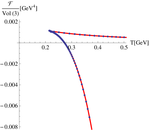
We show in Fig. 7 the free energy obtained by using the Bekenstein-Hawking entropy formula (full red line) as computed in this section, and the Einstein-Hilbert action (blue points) from Section 5, using NNLO terms in in Eq. (58) to compute the gluon condensate as a function of temperature. One clearly recognizes in this figure the first order phase transition at the temperature for zero flavours, which is quite close to lattice simulations. We consider the scale setting from the zero temperature gravity as a great success for gauge gravity duality. The upper branch in Fig. 7 represents the small black holes which are energetically disfavoured.
For high temperatures a weak coupling expansion of the pressure, , can be made. We refer the reader to Appendix B for a detailed discussion of the ultraviolet properties of the thermodynamic quantities. For an analytical computation in the ultraviolet, one makes a weak coupling expansion in . The coupling evaluated at the black hole horizon is finite. One can relate with the value of the running coupling at the scale by the following equation:
| (61) |
where is defined as indicated. The easiest way to compute the pressure from the entropy density is to solve the equation . Then one can consider a general scheme for the weak coupling expansion in the pressure, and solve for the coefficients in the above equation with given by Eq. (109). can be computed easily by making use of Eq. (111). Then one can identify the coefficients in the expansion. The result is
| (62) | |||||
where we show in the last expression the values of the coefficients corresponding to and .
In AdS/QCD we may choose the gravitational constant to reproduce the ideal gas limit at high temperatures, i.e. . Then one gets
| (63) |
We call the so determined constant indicating that it follows from the large temperature limit. As pointed out in Ref. [11], this value is a factor smaller than the value for super Yang-Mills theory. This decrease may be explained by the following two arguments. The number of degrees of freedom is reduced in QCD compared with SQCD by a factor . QCD is weakly interacting at high energies compared with the AdS/CFT theory which remains strongly interacting. This gives another factor .
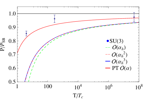
We show in Fig. 8 the pressure as a function of temperature, normalized to the Stefan-Boltzmann limit. It is noteworthy and visible in the figures that the expansion in terms of converge quite rapidly. On the other hand, as one can see the holographic model approaches the ultraviolet limit slower than lattice data. The asymptotic expansion of the pressure in QCD with has the form:
| (64) |
If one compares the coefficient in the ultraviolet expansion of the holographic model () Eq. (62) with the corresponding coefficient from perturbative QCD (), one gets a factor . This ratio explains the deviation observed in Fig. 8, since the leading coefficient gives a good approximation to lattice QCD at high temperatures . The same factor appears when one compares the first non-zero coefficient in the ultraviolet expansion of the trace anomaly which is , and so one expects that the holographic model also predicts values of larger than lattice data at high temperatures. This seems to be a property of the present holographic model, and there is no easy way to cure it. In Ref. [11] a behaviour for has been studied and numerical consistency between QCD and this AdS-model with a very simplified function is reached for . This parametrization disagrees, however, with the standard perturbative behavior of the -function of QCD, which has been the basic starting point to make AdS similar to QCD in the program of Refs. [21, 22, 10].
The parameterization presented in Ref. [15] is successful to reproduce lattice data in the regime , but in view of our analysis it is clear that this is because non perturbative effects are much stronger than perturbative ones even at very high temperatures, which seems to be not reasonable. As a matter of fact, the -function of Ref. [15] agrees only for with an accuracy with the asymptotic -function of QCD. The dilaton potential used in this reference has the correct uv-behaviour of QCD, but for all practical purposes it is a model potential which is designed to fit the thermal equation of the gluon plasma and not the -function established in perturbative QCD for . Since in Ref. [15] the scheme dependent term in the -function is very large, it is simply not clear how to determine the running of in the MOM or scheme from the parametrization of in this reference.
It is interesting to analyze the dependence of the phase transition temperature when the number of flavors is changed. The authors of Ref. [14] have studied the -dependence of the transition temperature with the help of renormalization group flow equations. As shown in this reference, the scale changes with . Therefore it is recommended to solve the Einstein equations by keeping the running coupling fixed at a mid scale , c.f. Eq. (23). In order to study the flavour dependence of in the present model, we vary the number of flavors from to in the coefficients and of the -function, c.f. Eqs. (8)-(9), which control the short distance (high temperature) regime. We retain the nonperturbative parameters and as in Eq. (11), which is reasonable because and are responsible for the infrared large distance (low temperatue) regime, and the string tension in the potential mainly depends on these two parameters. We don’t study the effect of dynamical quarks, therefore our analysis is restricted to a quenched approach.
Fig. 9 shows the dependence of the critical temperature on the number of flavors . Larger values of are difficult to implement numerically. We get for as transition temperature
| (65) |
which is very close to the lattice results [23]. It is gratifying that the absolute value of the transition temperature comes out so well inspite of the slow convergence of the pressure towards the Stefan-Boltzmann limit with increasing temperature. Comparing results with different flavour numbers we obtain an almost linear behaviour of the transition temperature for small :
| (66) |
This linear scaling of the critical temperature with for small has been claimed in Refs. [14, 24]. The value of we get is quite close to the one estimated in Ref. [14], . The flattening of the function for high values of in Fig. 9 is in accordance with Ref. [14]. This reference explains this fact as a consequence of the IR fixed-point structure of the theory. In our case the -function given by Eq. (4) does not have an IR fixed-point, and the flattening is a consequence of the weakening of the infrared coupling when increases. This means that it takes smaller scales to reach a critical coupling to bind the gluons into glueballs, and therefore has to decrease. We found that for the points plotted in Fig. 9, the value of is not affected much by .

7 Thermodynamic Observables independent of
We study in this section several thermodynamic quantities which are independent of the 5-d gravitational constant . For a more complete discussion of those thermodynamic quantities which dependent on we refer to Ref. [25].
First we focus on the speed of sound . From the specific heat per unit volume :
| (67) |
and the entropy density , one obtains the speed of sound:
| (68) |
A computation of this quantity in the ultraviolet leads to (see Appendix B for details)
| (69) |
In Fig. 10 we show the speed of sound computed with the holographic model, and compare the result with lattice data of Ref. [26]. We also plot the analytical ultraviolet approximation given in Eq. (69) including several orders in an expansion in . Since becomes close to in the calculation, we see that we have massless excitations in the plasma in the temperature range .

The spatial string tension is another quantity which is very useful to test AdS/QCD models. It is non-vanishing even in the deconfined phase, and it gives useful information about the non perturbative features of high temperature QCD. With a quark and an antiquark located at and respectively, the computation of the correlation function of rectangular Wilson loops in the plane leads to a potential between quark and antiquarks which behaves linearly at large distances, i.e.
| (70) |
For details on the computation we refer the reader to e.g. Ref. [27] and references therein. The spatial string tension takes the following form:
| (71) |
where is the string length. Making use of all the technology developed in Appendix B, we can easily compute the UV asymptotics of . Using the ultraviolet expansion of given by Eq. (102) and the corresponding expansion of given by Eq. (108), then Eq. (71) leads to
| (72) | |||||
We show in Fig. 11 a plot of as a function of temperature including several orders in Eq. (72), and the full numerical computation from Eq. (71). We show for comparison also the numerical result obtained from the model of Ref. [27]. One can see that our model reproduces very well the lattice data in the regime . A fit to the lattice data taken from Ref. [26] gives a good , and it is obtained by using which is larger than the value quoted in Ref. [1] based on a joint analysis of the heavy potential and running coupling at zero temperature. From a computation of the string tension at zero temperature one can see that this increase in can be partially explained as an effect of the change in the number of flavors, as Ref. [1] considers while we consider here . The string tension at can be computed as [27]
| (73) |
where gives the minimum of . Using the solution of and for , one reproduces the physical value for , while for one gets [1]. The discrepancy of with the value we get from the fit of is .

The vacuum expectation value of the Polyakov loop serves as an order parameter for the deconfinement transition in gluodynamics. The correlation function of two Polyakov loops taken in the large distance limit leads to the vacuum expectation value of one single Polyakov loop squared. This means that the Polyakov loop is related to the free energy of a single quark as
| (74) |
One of the main problems of the computation of this quantity is the renormalization. The multiplicative renormalizability of the Polyakov loop was first established in Ref. [28]. The Polyakov loop was computed in perturbation theory for the first time in Ref. [29] in pure gluodynamics. There has been recent progress to renormalize it in the lattice following different methods based on the computation of the one point and two point correlation functions of Polyakov loops. The multiplicative renormalization is then reached by identifying and extracting the quark self energy, see e.g. Refs. [30, 31]. In Ref. [32] it was proposed by one of the authors a phenomenological ansatz based on a dimension two gluon condensate of the dimensionally reduced effective theory of QCD, which was quite successful to reproduce lattice data of the Polyakov loop in the deconfined phase down to . 11 1 See also Refs. [33, 34] for an application of this ansatz to compute the heavy quark-antiquark free energy and the equation of state of QCD. This ansatz follows from the observation for the first time in Ref. [32] that close and above the behavior of the Polyakov loop is characterized by power corrections in . These power corrections were later observed also in the equation of state of gluodynamics [35]. The computation of the Polyakov loop within the AdS/QCD formalism was addressed recently in Ref. [36] within a model based on a specific choice of the warp factor which naturally introduces these power corrections. In the following we will consider this approach, but using our model dictated by the 5-d grativy action.
One can compute the vacuum expectation value of the Polyakov loop from the Nambu-Goto action of a string hanging down from a static quark on the boundary into the bulk. 22 2 The coupling of the two dimensional curvature to the dilaton field is a well known correction to the Polyakov action which propagates to the Nambu Goto action [37]. In first order it enters there by a modified non conformal metric, as it is considered here. Higher order terms are interesting to investigate, but are in the scope of a separate longer study. The fundamental string is stretched between the test quark at the boundary () and the horizon () of the black hole solution. See Ref. [36] for details. The Nambu-Goto action then reads
| (75) |
The action Eq. (75) is divergent at . One can regularize it by substracting the action of the thermal gas solution up to a cutoff :
| (76) | |||||
The cutoff becomes necessary because the free energy of a single quark diverges at . Note that introduces a normalization constant into the free energy . In the second equality of Eq. (76) we have divided the action corresponding to the thermal gas solution into two integrals. The first integral inside the bracket in Eq. (76) is UV convergent, as zero and finite temperature solutions have the same behavior in the UV. The renormalized vacuum expectation value of the Polyakov loop then writes
| (77) |
defined in Eq. (76) tends to zero in the limit independently of the value of , and so tends to . We show in Figure 12 as a continuous black line the behavior of as a function of temperature computed numerically from Eqs. (76)-(77), and its comparison with lattice data for gluodynamics with taken from Ref. [31]. In order to reproduce lattice data, we have performed a fit by considering the string length and the cutoff as free parameters. The best fit in the regime leads to
| (78) |
Note that is larger than the value we used for the spatial string tension, but it differs just from the value one needs to reproduce the string tension at (see Eq. (73) and discussion below). Our approach fits the Polyakov loop very well without a dimension two condensate, since a dimension two operator would show up in the ultraviolet expansion of the thermal solutions near , Eqs. (46)-(49). This does not exclude that a good fit to the data exists of the form with , , in accordance with Ref. [32] (see also Ref. [36]). The Polyakov loop is zero in the confined phase and our approach gives a nonzero value at given by . This first order jump is similar to the one predicted by the more reliable lattice data , c.f. Fig. 12.

We compute in details in Appendix B the UV asymptotics of the Polyakov loop. The results is
| (79) |
We show in Fig. 12 the analytical result given by Eq. (79), using the value of quoted in Eq. (78). The Polyakov loop was computed in perturbative QCD up to NLO in Ref. [29] (see also Ref. [32]), and it has been recently corrected by two groups Ref. [38, 39]. For gluodynamics this gives
| (80) |
Note that since the perturbative -function starts at order , changes in the scale affect . In Eq. (79) the power counting in doesn’t follow the perturbative scheme. This discrepancy with PT is common of all the renormalization group revised models constructed by the general procedure of Kiritsis et al., c.f. Refs. [22, 21]. We have plotted in Fig. 12 also the perturbative result given by Eq. (80). Note that lattice data approach the perturbative result very accurately for above . Here the AdS-perturbation theory does not seem to converge rather rapidly.
8 Discussion and final remark
We have demonstrated in this work the numerical agreement between computations of the free energy from the Einstein-Hilbert action and from the Bekenstein-Hawking entropy formula. Both approaches leads to the same result, but the former method is much more sensitive to numerical errors, and an accurate computation is only possible when one takes care of including leading logarithmic effects in an ultraviolet expansion of the scale factor at finite temperature.
We have also computed analytical expressions in the ultraviolet for the thermodynamic quantities as an expansion in powers of the running coupling evaluated at the black hole horizon. This expansion turns out to converge quite rapidly even at temperatures , quite opposite to the conventional QCD perturbation theory at high temperature [40]. We have extended our analysis to other thermodynamic quantities computed in the string frame, in particular the spatial string tension and the vacuum expectation value of the Polyakov loop, and the agreement with lattice data is better in this case.
From our analysis we see that the gravity model cannot reproduce at the same time lattice data of the equation of state of the gluon plasma at very high temperatures, and close to the phase transition. This means that fixing the gravity constant from the ideal gas limit seems not to be consistent with thermodynamics close to the phase transition. In this sense, there is the possibility that the ideal gas limit doesn’t correspond to the limit of the black hole gravity theory at high temperatures. Is it possible that the gravity theory allows more degrees of freedom at high temperatures? Or is the simulation of higher terms in the string coupling in the gravity action incomplete? Since the agreement of the velocity of sound, the spatial string tension and the Polyakov loop in the string frame is better, the question arises whether the gravity action approximates the string action truthfully. We will further address this problem, and analyze possible solutions [41] in forthcoming work.
The approach presented here and in previous references, see e.g. Refs. [10, 11], is a phenomenological gravity theory motivated by non-critical string theory. The results are subject to corrections and one can only hope that they capture the expected -function behavior. It has to be mentioned also as a caveat that the contribution of the coupling of the world-sheet to the dilaton field may very well change the quantitative, and even the qualitative result substantially. This should be checked in future works.
Acknowledgments:
E.M. would like to thank the Humboldt Foundation for their stipend. This work was also supported in part by the ExtreMe Matter Institute EMMI in the framework of the Helmholtz Alliance Program of the Helmholtz Association. We thank D. Antonov, R.D. Pisarski, E. Ruiz Arriola and A. Vairo for useful comments on the manuscript.
Appendix A: Numerical solution of Einstein equations for the black hole metric
In this appendix we discuss in details the procedure to solve numerically the system of Einstein equations given by Eqs. (38)-(41). A numerical solution of the system demands a good starting point. The boundary at has the disadvantage that is singular at this point. The horizon at is not a good expansion point either, since the inverse of the black hole factor is singular there. Practically it is possible to start at some value close to the horizon, . The initial values can then be expanded in terms of their values at the horizon as
| (81) | |||
| (82) | |||
| (83) | |||
| (84) | |||
| (85) |
where we use the notation
| (86) |
From Eqs. (84), (85) and one can derive and its derivatives. The expression for follows from Eq. (38) by applying l’Hôpital rule in the second term of the r.h.s. To compute the expression of the second derivative , one derives Eq. (38) with respect to once, and uses the result of . The result is
| (87) | |||
| (88) | |||
| (89) |
where we have defined for simplicity of notation
| (90) |
and
| (91) |
The derivative of with respect to , i.e. , can be computed analytically from the analytical expression of , c.f. Eq. (6).
Our procedure to solve the system of first order differential equations Eqs. (38)-(41) follows Refs. [15, 42]. First we choose arbitrary values for the functions at the horizon, namely
| (92) |
and the initial values for temperature and ,
| (93) |
We rewrite the initial conditions, Eqs. (81)-(85), in the coordinate, so that and . The parameter is chosen very small, such that is very close to and the initial conditions are accurate enough. The variables , differ from , by a rescaling factor. Then one integrates numerically the system to get solutions , , and in some interval , where diverges at . Since the system of equations (38)-(41) is invariant under three different rescalings [15], one can make use of these properties to find a solution which has the right boundary conditions. In step 2, one shifts the coordinate, so that the ultraviolet divergence of is at the origin. The new solution reads
| (94) |
In step 3, one chooses in such a way that , which is the correct value of in the UV,
| (95) |
Finally one rescales :
| (96) |
The value is determined by comparing the zero temperature metric and the finite temperature metric at a point which has the same ultraviolet coupling as the zero temperature solution. In practice we choose . Then the rescaling factor is given as
| (97) | |||||
| (98) | |||||
| (99) |
Starting from the values of , and mentioned above, one gets
| (100) |
By this procedure the QCD-parameter in the asymptotic logarithms of both solutions also agree. Because , the operations performed in Eqs. (94)-(96) rescales the value of to the right temperature T,
| (101) |
From Eqs. (100), (101) and the value one gets . In practice we solve the equations of motion for different temperatures by choosing different values for . Note that is invariant under the set of rescaling Eqs. (94)-(96).
Appendix B: Ultraviolet properties of the thermodynamic quantities
We will study in this appendix the analytical properties of the thermodynamic quantities in the ultraviolet. 33 3 In this analysis we will explicitly show every expression including all the perturbative orders one needs to compute the thermodynamic quantities up to . Being the UV expansion of given by (c.f. Eq. (29))
| (102) |
the entropy can be computed by evaluating the above expression at the horizon, i.e. by computing . The information on the horizon is given by the function , and so one should study its behavior in the UV. Combining Eqs. (39) and (41) one gets
| (103) |
Given one can solve this equation to get . Two integration constants are needed, which as usual are chosen by imposing the boundary conditions and [10]. The result for the UV asymptotics of is
| (104) |
where
| (105) |
and is given by Eq. (26). One can arrive at this result by considering the explicit expression of given by Eq. (102), insert it into Eq. (103) and solve the equation reexpressing the result in powers . A much easier way to arrive at this result is to consider a general scheme , and then introduce it and Eq. (102) into Eq. (103). The derivative of is given by
| (106) |
This useful relation can be proved easily from the explicit expression of , c.f. Eq. (26). Using Eq. (106), the equation of motion Eq. (103) can be expressed in powers of , and one can easily identify the coeficients , , , , which fulfill the equation. The result is given by Eqs. (104) and (105).
From Eq. (104) and using Eq. (106), the derivative of then evaluates to
| (107) | |||||
The temperature is obtained by evaluating the above expression at the horizon
| (108) |
We have corrected some error in the computation of Ref. [10], where the authors consider a factor instead of at order in the bracket of Eq. (108).
The entropy density easily follows by evaluating Eq. (102) at the horizon, and using the relation between and given by Eq. (108). Then one gets
| (109) | |||||
which corresponds to the weak coupling expansion of the entropy. To deal with Eq. (109) one needs to know the temperature dependence of . Taking into account the relation between and given by Eq. (108), it can be proved that 44 4 Note that because of Eq. (110) the expressions of the thermodynamics quantities up to remain valid when one substitutes by .
| (110) |
where is defined as indicated. One can prove that by using the explicit expansion given by Eq. (26). By considering in Eq. (106) one gets 55 5 The definition of given in Eq. (110) doesn’t agree with the usual definition of the running coupling at finite temperature, for which the prescription is usually taken. Both prescriptions differ at , i.e. , as it is evident from Eq. (111).
| (111) |
The version of this formula easily follows by considering Eq. (110). Eq. (111) is very useful, and it can be used for instance to compute easily the pressure from Eq. (109) (see Section 6 for a discussion). The energy density follows trivially from Eqs. (109) and (62)
| (112) | |||||
Note that in the weak coupling expansion of the thermodynamics quantities, Eqs. (109), (62) and (112), there are no half-integer powers in , i.e. , , as we don’t consider loops contributions, in contrast to the weak coupling expansion in QCD [40]. These results extend to the results of Ref. [10]. From the energy density and pressure one can compute the trace anomaly. It reads
| (113) |
The trace anomaly is related to the vacuum expectation value of the gluon condensate. As it was pointed out in Ref. [10] and discussed by us in Sec. 4, the gluon condensate appears in the UV expansion of the difference between the black-hole and zero temperature solutions, c.f. Eqs. (46)-(49). In this Appendix we have not taken into account power corrections in . However, just by computing using Eq. (46), it is straightforward to prove that the correction induces a contribution in , , and , and so this corresponds to much a lower order contribution in the UV expansion performed previously. By the same way, the power correction in induces a correction in which is subleading in our UV analysis, and so it is enough to identify with at this level, as it has been done in previous formulas.
From previous analysis we can derive easily the expressions for the weak coupling expansion of the specific heat per unit volume
| (114) | |||||
and speed of sound
| (115) |
Eq. (114) follows by using Eqs. (111) and (62), while Eq. (115) is obtained from Eqs. (109) and (114).
For completeness of this apendix, we study the high temperature behavior of the Polyakov loop. At the end one wants to express the result as an expansion in powers of , and the easiest way to proceed is to work in coordinates dependent on the running coupling as a variable, instead of . The relation between and is given by [1]
| (116) |
where the function reads
| (117) |
Using Eqs. (116), one can rewrite the Nambu-Goto action which involves an integration in , Eq. (75), as
| (118) |
In the intermediate steps we will make use explicitly of the UV -function up to 4-loops order just for completeness, i.e.
| (119) |
but our final result of the Polyakov loop up to will depend only on and , c.f. Eq. (124). Inserting the UV -function, Eq. (119), into Eq. (117), one gets
| (120) |
Note that Eq. (116) combined with the expansions of and given by Eqs. (102) and (120) respectively, leads to Eq. (106). The main difficulty is to express as a function of . The UV expansion of is given by Eq. (102). To compute one has to invert Eq. (26). The result is
| (121) | |||||
From Eqs. (102) and (121), one gets
| (122) | |||||
Then inserting Eqs. (120) and (122) into Eq. (118), and performing the integration in , one arrives at
| (123) |
where is divergent and comes from the lower limit in the integration. To arrive at Eq. (123) one has to make use of Eq. (121) evaluated at the horizon, and use the relation between and given by Eq. (108). Then the renormalized vacuum expectation value of the Polyakov loop writes
| (124) |
where . Note that tends to from above in the high temperature limit, which is the behavior predicted by standard perturbative QCD.
References
- [1] B. Galow, E. Megias, J. Nian, and H. J. Pirner, Nucl. Phys. B834, 330 (2010), 0911.0627.
- [2] D. Antonov, H. J. Pirner, and M. G. Schmidt, Nucl. Phys. A832, 314 (2010), 0808.2201.
- [3] J. Polchinski and Z. Yang, Phys. Rev. D46, 3667 (1992), hep-th/9205043.
- [4] M. C. Diamantini and C. A. Trugenberger, Phys. Rev. Lett. 88, 251601 (2002), hep-th/0202178.
- [5] I. I. Kogan and A. Kovner, (2002), hep-th/0205026.
- [6] G. Policastro, D. T. Son, and A. O. Starinets, Phys. Rev. Lett. 87, 081601 (2001), hep-th/0104066.
- [7] J. Erdmenger, N. Evans, I. Kirsch, and E. Threlfall, Eur. Phys. J. A35, 81 (2008), 0711.4467.
- [8] D. Mateos, R. C. Myers, and R. M. Thomson, Phys. Rev. Lett. 97, 091601 (2006), hep-th/0605046.
- [9] H. J. Pirner and B. Galow, Phys. Lett. B679, 51 (2009), 0903.2701.
- [10] U. Gursoy, E. Kiritsis, L. Mazzanti, and F. Nitti, JHEP 05, 033 (2009), 0812.0792.
- [11] J. Alanen, K. Kajantie, and V. Suur-Uski, Phys. Rev. D80, 126008 (2009), 0911.2114.
- [12] S. W. Hawking and D. N. Page, Commun. Math. Phys. 87, 577 (1983).
- [13] J. D. Bekenstein, Phys. Rev. D7, 2333 (1973).
- [14] J. Braun and H. Gies, JHEP 05, 060 (2010), 0912.4168.
- [15] U. Gursoy, E. Kiritsis, L. Mazzanti, and F. Nitti, Nucl. Phys. B820, 148 (2009), 0903.2859.
- [16] http//wwwtheory.lbl.gov/ianh/alpha/alpha.html.
- [17] A. A. Vladimirov, Sov. J. Nucl. Phys. 31, 558 (1980).
- [18] S. Carlip, Lect. Notes Phys. 769, 89 (2009), 0807.4520.
- [19] G. W. Gibbons and S. W. Hawking, Phys. Rev. D 15, 2752 (1977).
- [20] G. Endrodi, Z. Fodor, S. D. Katz, and K. K. Szabo, PoS LAT2007, 228 (2007), 0710.4197.
- [21] U. Gursoy and E. Kiritsis, JHEP 02, 032 (2008), 0707.1324.
- [22] U. Gursoy, E. Kiritsis, and F. Nitti, JHEP 02, 019 (2008), 0707.1349.
- [23] B. Beinlich, F. Karsch, E. Laermann, and A. Peikert, Eur. Phys. J. C6, 133 (1999), hep-lat/9707023.
- [24] J. Braun, Phys. Rev. D81, 016008 (2010), 0908.1543.
- [25] E. Megias, H. J. Pirner, and K. Veschgini, Nucl. Phys. Proc. Suppl. 207-208, 333 (2010), 1008.4505.
- [26] G. Boyd et al., Nucl. Phys. B469, 419 (1996), hep-lat/9602007.
- [27] J. Alanen, K. Kajantie, and V. Suur-Uski, Phys. Rev. D80, 075017 (2009), 0905.2032.
- [28] A. M. Polyakov, Nucl. Phys. B164, 171 (1980).
- [29] E. Gava and R. Jengo, Phys. Lett. B105, 285 (1981).
- [30] O. Kaczmarek, F. Karsch, P. Petreczky, and F. Zantow, Phys. Lett. B543, 41 (2002), hep-lat/0207002.
- [31] S. Gupta, K. Huebner, and O. Kaczmarek, Phys. Rev. D77, 034503 (2008), 0711.2251.
- [32] E. Megias, E. Ruiz Arriola, and L. L. Salcedo, JHEP 01, 073 (2006), hep-ph/0505215.
- [33] E. Megias, E. Ruiz Arriola, and L. L. Salcedo, Phys. Rev. D75, 105019 (2007), hep-ph/0702055.
- [34] E. Megias, E. Ruiz Arriola, and L. L. Salcedo, Phys. Rev. D80, 056005 (2009), 0903.1060.
- [35] R. D. Pisarski, Prog. Theor. Phys. Suppl. 168, 276 (2007), hep-ph/0612191.
- [36] O. Andreev, Phys. Rev. Lett. 102, 212001 (2009), 0903.4375.
- [37] E. Kiritsis, Princeton, USA: Univ. Pr. (2007) 588 p.
- [38] Y. Burnier, M. Laine, and M. Vepsalainen, JHEP 01, 054 (2010), 0911.3480.
- [39] N. Brambilla, J. Ghiglieri, P. Petreczky, and A. Vairo, Phys. Rev. D82, 074019 (2010), 1007.5172.
- [40] K. Kajantie, M. Laine, K. Rummukainen, and Y. Schroder, Phys. Rev. D67, 105008 (2003), hep-ph/0211321.
- [41] E. Megias, H. J. Pirner, and K. Veschgini, in preparation (2011).
- [42] J. Alanen, K. Kajantie, and K. Tuominen, Phys. Rev. D82, 055024 (2010), 1003.5499.