darkredrgb.7,0,0 \definecolorgreenrgb0,0.7,0
Multiscale Modelling and Inverse Problems
Abstract
The need to blend observational data and mathematical models arises in many applications
and leads naturally to inverse problems. Parameters appearing
in the model, such as constitutive tensors, initial conditions, boundary conditions, and forcing can be estimated on the basis of observed data. The resulting inverse problems are often ill-posed and some form of regularization is required.
These notes discuss parameter estimation in situations where the unknown parameters vary across multiple scales. We illustrate the main ideas using a simple model for groundwater flow.
We will highlight various approaches to regularization
for inverse problems,
including Tikhonov and Bayesian methods.
We illustrate three ideas that arise when considering
inverse problems in the multiscale context. The
first idea is that the choice of space or set in which to
seek the solution to the inverse problem is intimately related to
whether a homogenized or full multiscale
solution is required. This is a choice of regularization.
The second idea is that, if a homogenized solution
to the inverse problem is what is desired, then this
can be recovered from carefully designed
observations of the full multiscale system.
The third idea is that the theory of
homogenization can be used to improve the estimation
of homogenized coefficients from multiscale data.
1 Introduction
The objective of this overview is to demonstrate the important role of multiscale modelling in the solution of inverse problems for differential equations. The main inverse problem we discuss is that of determining unknown parameters by matching observed data to a differential equation model involving those parameters. The unknown parameters may be functions, in general, and they may have variation over multiple (length) scales. This multiscale structure makes the forward problem more challenging: numerically computing the solution to the differential equation requires very high resolution. The multiscale structure also complicates the inverse problem. Should we try to fit the data with a high-dimensional parameter, or should we seek a low-dimensional “homogenized” approximation of the parameter? If a low-dimensional parameter model is used, how should we account for the mismatch between the true parameters and the low-dimensional representation? After obtaining a solution to the inverse problem, one typically wants to make further predictions using whatever parameter is fit to the observed data, so it is important to consider whether a low-dimensional representation of the unknown parameter is sufficient to make additional predictions.
Throughout these notes the unknown parameters will be denoted by ; typically is a function assumed to lie in a Banach space . We use to denote the data (for simplicity we often take ) and to denote the predicted quantity, assumed to be an element of a Banach space or, in some cases, a valued random variable. The map denotes the forward mapping from the unknown parameter to the data, and (or in the random case) denotes the forward mapping from the parameter to the prediction. We sometimes refer to as the observation operator and as the prediction operator. Both and are typically derived from a common solution operator mapping to the solution of a partial differential equation (PDE), where is a Banach space. For example may be derived by composing with linear functionals.
The ideal inverse problem is to determine from knowledge of where it is assumed that In practice, however, the data is generated from outside this clean mathematical model, so it is natural to think of the data as being given by
| (1) |
for some quantifying model error11 1 Model error can be incorporated within the set of unknown parameters and estimated using data; however this idea is not pursued here. and observational noise. The value of is not known, but it is common in applications to assume that some of its statistical properties are known and these can then be built into the methods used to estimate . Once the function is determined by solving this inverse problem, it can be used to make a prediction
We illustrate three ideas that arise when attempting to solve the inverse problem defined by (1) in the multiscale context:
- •
(a) The choice of the space or set in which to seek the solution to the inverse problem is intimately related to whether a low-dimensional “homogenized” solution or a high-dimensional “multiscale” solution is required for predictive capability. This is a choice of regularization.
- •
(b) If a homogenized solution to the inverse problem is desired, then this can be recovered from carefully designed observations of the full multiscale system.
- •
(c) The theory of homogenization can be used to improve the estimation of homogenized parameters from observations of multiscale data.
In Section 2 we consider in detail a worked example which exemplifies the use of multiscale methods to approximate the forward problems and for data and predictions; this example will be used to illustrate many of the general ideas developed in these notes, and the three ideas (a)–(c) in particular. Section 3 is devoted to a brief overview of regularization techniques for inverse problems, and to discussion of the idea (a). Section 4 is devoted to the idea (b). We study the problem of estimating a single scalar parameter in a homogenized model of groundwater flow, given data which is generated by a full multiscale model. This may be seen as a surrogate for understanding the use of real-world data (which is typically multiscale in character) to estimate parameters in simpler homogenized models. Section 5 is devoted to the idea (c). We study the use of ideas from multiscale methodology to enhance parameter estimation techniques for homogenized models. The viewpoint taken is that the statistics of the error appearing in (1) can be understood using the theory of homogenization for random media; when these statistical properties depend on the unknown parameter the noise is no longer additive and its dependence on plays an important role in the parameter estimation process.
1.1 Notation
The following notation will be used throughout. We use to denote the Euclidean norm on (for possibly different choices of ). We let (resp. ) denote the set of symmetric (resp. positive-definite) second order tensors on . If , we define the weighted norm on . Throughout the notes, is a Banach space, containing the functions that we wish to estimate, and a Banach space compactly embedded into . When studying the inverse problem from a Bayesian perspective we will use Gaussian priors on , defined via a covariance operator on a Hilbert space , with norm . In this situation will be the Hilbert space with norm .
1.2 Running Example
We consider a model for groundwater flow in a medium with permeability tensor , pressure and Darcy velocity (or the volume flux of water per unit area) related to the pressure via the Darcy law:
| (2) |
where is the fluid viscosity, is the fluid density, is the acceleration due to gravity and is the unit vector in the -direction. We choose units in which We also assume that we have a constant density fluid and redefine the pressure by adding ( is the vertical direction) to write (2) in the form . Assuming that the Darcy velocity is divergence-free, except at certain known source/sink locations, we obtain the following elliptic equation for the pressure:
| (3) | ||||
where is an open and bounded set with regular boundary, and is assumed to be known. The permeability tensor field , however, is assumed to be unknown and must be determined from data. In order to make the elliptic PDE (3) for the pressure well-posed, we assume that the permeability tensor is an element of and so we write it as the (tensor) exponential: , . It is natural to view as an element of and to consider weak solutions of (3) with Then we have a unique solution satisfying
| (4) |
for some depending only on and , and being the essential supremum of the spectral radius of the matrix , as varies over :
Thus we may define by Now consider a set of real-valued continuous linear functionals and define by The inverse problem is to determine from where it is assumed that is given by (1). Using (4) one may show that (resp. ) is Lipschitz. Indeed if denotes the solution to (3) with log permeability then, we have
| (5) |
Study of the transport of contaminants in groundwater flow is a natural example of a useful prediction that can be made once the inverse problem is solved. To model this scenario we consider a particle which is advected by the the groundwater velocity field , where is the porosity of the rock and is the Darcy velocity field from (3), and subject to diffusion with coefficient Assuming that the contaminant is initially at we obtain the stochastic differential equation (SDE):
| (6) |
where is a standard Brownian motion on . If we are interested in predicting the location of the contaminant at time then our prediction will be the function given by Here for each fixed the function maps into the family of valued random variables.
2 The Forward Problem: Multiscale Properties
Some inverse problems arising in applications have the property that the forward model mapping the unknown to the data will produce similar output on both highly oscillatory functions and on appropriately chosen smoothly varying functions . Furthermore, for some choices of prediction function the predictions themselves will also be close for both highly oscillatory functions and on appropriately chosen smoothly varying functions . These properties can be seen from an application of multiscale analysis, and we illustrate them by considering the problem introduced in Section 1.2. There are many texts on the theory of multiscale analysis. For example, the basic homogenization theorems discussed here are developed in [6]. A recent overview of the subject, with many other references and using the same notational conventions that we adopt here, is [24].
We consider a multiscale version of the running example from Section 1.2 where the permeability tensor is where is periodic in the second argument, a small parameter. For now we have assumed periodic dependence on the fast scale in ; however we will generalize this to random dependence in later developments.
With this permeability we obtain the family of problems
| (7a) | |||||
| (7b) | |||||
| (7c) | |||||
If we set , then the transport of contaminants is given by the SDE
| (8) |
Standard techniques from the theory of homogenization for elliptic PDEs can be used to show that for small,
| (9) |
where and are defined as follows. First we define the effective (homogenized) permeability tensor via solution of the cell problem for :
| (10) |
Then
| (11) | ||||
| (12) |
In this sense we observe that the effective diffusivity is the average of over the fast scale . This is not equal to the average of over , except in trivial cases. We denote by the logarithm of so that
The function solves the ( independent) elliptic PDE
| (13a) | |||||
| (13b) | |||||
| (13c) | |||||
and the corrector is given by
| (14) |
Note that (10) may be written as
| (15) |
This shows that , which is averaged to give the effective permeability tensor, is divergence-free with respect to the fast variable
It is possible to prove that, in the limit as , solutions to (7) converge to solutions to (13), the convergence being strong in and weak in [10, 1, 24]. However if we want to prove strong convergence in then we need to include information about the corrector term . The following theorem and corollary summarize these ideas. For proofs see [1], or the discussion in the texts [10, 24].
Corollary 1
In fact it is frequently the case that the convergence in Theorem 16 may be obtained in a stronger topology. Reflecting this we make the following assumption.
Assumption 2.2
The function converges to in and its gradient converges to the gradient of in so that
In Appendix Appendix 2 we prove this assumption for the one dimensional version of (7). The proof in the multidimensional case will be presented elsewhere [22]. The proof of this assumption in the multidimensional case is based on the estimates proved in [2] (in particular, Lemma 16), see also (15, Lemma 2.1).
With these limiting properties of the elliptic problem (7) at hand it is natural to ask what is the limiting behaviour of governed by (8). To answer this question we define
| (17) |
Notice that this ordinary differential equation (ODE) has vector field which is defined entirely through knowledge of the homogenized permeability : once is known, the elliptic PDE (13) can be solved for and then is recovered from (13c). If we can show that solutions of (8) and (17) are close then this will establish that the prediction of particle transport in the model (7), (8) can be made accurately by use of only homogenized information about the permeability.
In proving such a result there are a number of technical issues which arise caused by the presence of the boundary of the domain in which the PDE (7) is posed. In particular solutions of (8) may leave requiring a definition of the velocity field outside . These issues disappear if we consider the case where is itself a box of length and is equipped with periodic boundary conditions instead of Dirichlet conditions: we may then extend all fields to the whole of by periodicity. In this case, the homogenization theory for (7) with (7b) replaced by periodic boundary conditions is identical to that given above, except that (13b) is also replaced by periodic boundary conditions. We write and adopt this periodic setting for the next theorem, which is proved in Appendix Appendix 1:
Theorem 2.3
In summary, this example exhibits the property that, if the length scale is small, the data generated from and may appear very similar due to homogenization effects. Therefore, when trying to infer parameters from data, it is difficult to distinguish between and without some form of regularization or prior assumptions about the form of the parameter. On the other hand, Theorem 2.3 shows that knowing only is sufficient to make accurate predictions of the trajectories of (8).
3 Regularization of Inverse Problems
In this section we describe various approaches to regularizing inverse problems, motivating them by reference to the multiscale example in the previous section. The approach to regularizing which is described in Section 3.2 is developed in detail in [5]. The Tikhonov regularization approach from Section 3.3 is developed in detail in [16, 17]. Both of these regularization approaches are specific examples of the general set-up often called PDE constrained optimization, which we discuss in Section 3.4; this subject is overviewed in [18]. An overview of the Bayesian approach to inverse problems, a subject that we outline in Section 3.5, is given in [26] and [17].
3.1 Set-Up
Our objective here is to determine , given , where and are related by (1). We assume that, whilst the actual value of is not available, it is reasonable to view it as a single draw from a statistical distribution whose properties are known to us. To be concrete we assume that is drawn from a mean zero Gaussian random variable with covariance : we write this as . We make the following continuity assumption concerning the observation operator . Note that this (local) Lipschitz condition also implies an (exponential in ) bound on
Assumption 3.1
There are constants such that, for with ,
In general the inverse problems such as that given by (1) with are hard to solve: they may have no solutions, multiple solutions and solutions may exhibit sensitive dependence on initial data. For this reason it is natural to seek a least squares approach to finding functions which best explain the data. In view of the assumed structure on a natural least squares functional is
| (18) |
The weighting by in the Euclidean norm induces a normalization on the model-data mismatch. This normalization is given by the assumed standard deviations of the noise in a coordinate system defined by the eigenbasis for .
Example 1
Consider the running example of Section 1.2. Equation (5) shows that Assumption 3.1 holds in this case, noting that for some linear functional on , with the choice , provided . We use this example to illustrate why inverse problems are, in general, hard.
Assume that the linear functionals satisfy the property that as This occurs if they are linear functionals on , by Theorem 16 or if Assumption 2.2 holds, if they are linear functionals on Writing this in terms of we have as (Note that this occurs even though and are not themselves close.) Hence there is an uncountable family of functions (indexed by all sufficiently small) which all return approximately the same value of and thus simply minimizing may be very difficult. Furthermore, there may be minimizing sequences which do not converge. For example fix a particular realization of the data given by where is the homogenized log permeability. Then for all and as , since
| (19) |
On the other hand, does not converge in as .
∎
In order to overcome the difficulties demonstrated in this example regularization is needed. In the remaining sections we discuss various regularizations, in general, illustrating ideas by returning to the running example.
3.2 Regularization by Minimization Over a Convex, Compact Set
Recall that is a Banach space compactly embedded into . Let Then is a closed convex and bounded set in and, as such, any sequence in must contain a weakly convergent subsequence with limit in (see, for example, Theorem 1.17 in [18]). Now consider the minimization problem
| (20) |
Theorem 3.2
Any minimizing sequence for (20) contains a weakly convergent subsequence in with limit which attains the infimum:
Proof.
This is a classical theorem from the field of optimization; see [18] for details and context. Since is contained in we deduce the existence of a subsequence (which for convenience we relabel as ) with weak limit Thus in . Hence, by compactness, in . By Assumption 3.1 we deduce that is weakly continuous. By definition, for any there exists such that
By weak continuity of we deduce that
The result follows since is arbitrary. ∎∎
Example 2
Consider the running example of Section 1.2. Let denote a fixed symmetric positive-definite tensor so that is defined. We define the subspace of tensor valued functions of the form , for some constant noting that then . By Lipschitz continuity of in we deduce (abusing notation) Lipschitz continuity of viewed as a function of . We define
| (21) |
We may take the norm Thus the problem (20) attains its infimum for some . The regularization of seeking to minimize over corresponds to looking for solution over a one-parameter set of tensor fields, in which the free parameter is bounded by Note that such a solution set automatically rules out the oscillating minimizing sequences which were exhibited in Example 1. ∎
3.3 Tikhonov Regularization
Instead of regularizing by seeking to minimize over a bounded and convex subset of a compact set in , we may instead adopt the Tikhonov approach to regularization. We consider the minimization problem
| (22) |
where
| (23) |
Theorem 3.3
Any minimizing sequence for (22) contains a weakly convergent subsequence in with limit which attains the infimum:
Proof.
This is a classical theorem from the calculus of variations; see [12] for details and context. Since is a minimizing sequence and , we deduce that for any there exists such that
From this it follows that is bounded in and hence contains a weak limit , along a subsequence which, for convenience, we relabel as . The weak continuity of , together with weak lower semicontinuity of the function implies the weak lower semicontinuity of . Hence
Since , the result follows. ∎∎
Example 3
Consider the running example of Section 1.2. Let and note that is compact in for Thus the problem (22) attains its infimum for some . As with the example from the previous section the regularization rules out highly oscillating minimizing sequences such as those seen in Example 1. The choice of the parameter will effect how much oscillation is allowed in any minimizing sequence. ∎
3.4 PDE Constrained Optimization
The regularizations imposed in the two previous subsections involed the imposition of constraints on the input to a PDE model and the resulting minimizations were expressed in terms of alone. For at least two reasons it is sometimes of interest to formulate the minimization problem simultaneously over the input variable , together with the solution of the PDE : firstly computational algorithms which work to find in can be more effective than working entirely in terms of ; and secondly regularization constraints may be imposed on the variable as well as on If then this leads to constrained minimization problems of the form
| (24) |
where denotes the constraints imposed on both the input and on the output from the PDE model. Typically the observation operator is found from and then the information in can be built into the definition of .
Example 4
Consider the running example from Section 1.2 and assume that the observational noise Define
for some Choosing and , together with and we obtain from (24) the minimization from Example 3 in the case Choosing , and from Example 2 we recover that example. Choosing and/or choosing the constraint set to impose constraints on leads to minimization in which the output of the PDE model is constrained as well as the input that we are trying to estimate. ∎
3.5 Bayesian Regularization
The preceding regularization approaches have a nice mathematical structure and form a natural approach to the inverse problem when a unique solution is to be expected. But in many cases it may be interesting or important to find a large class of solutions, and to give relative weights to their importance. This allows, in particular, for predictions which quantify uncertainty. The Bayesian approach to regularization does this by adopting a probabilistic framework in which the solution to the inverse problem is a probability measure on , rather than a single element of .
We think of as a random variable. Our goal is to find the distribution of given , often denoted by . We define the joint distribution of as follows. We assume that and appearing in (1) are indepenent mean zero Gaussian random variables, supported on and respectively, with covariance operator and covariance matrix respectively. By equation (1), the distribution of given , denoted , is Gaussian . The measure is known as the prior measure. It is most natural to define the measure on a Hilbert space . Under suitable conditions on , we have . This means that under the measure , almost surely so that is well-defined, almost surely. If , it follows that the Hilbert space with norm is compactly embedded into The space is known as the Cameron-Martin space. In the infinite dimensional setting, functions drawn from are almost surely not in the Cameron-Martin space. See [9, 20] for detailed discussion of Gaussian measures on infinite dimensional spaces.
When solving the inverse problem, the aim is to find the posterior measure and to obtain information about likely candidate solutions to the inverse problem from it. Informal application of Bayes’ theorem gives
| (25) |
The probability density function for is, using the property of Gaussians, proportional to
The infinite dimensional analogue of this result is to show that is absolutely continuous with respect to with Radon-Nikodym derivative relating posterior to prior as follows:
| (26) |
Here is given by (18) and The meaning of the formula (26) is that expectations under the posterior measure can be rewritten as weighted expectations with respect to the prior: for a function on we may write
Theorem 3.4
If are probability measures that are absolutely continuous with respect to the probability measure , then the Hellinger metric is defined as
For any function of which is square integrable with respect to both and it may be shown that the difference in expectations of that function, under and under , is bounded above by the Hellinger distance. In particular, this theorem shows that the posterior mean and covariance operators corresponding to data sets and are apart.
The choice of prior , relates directly to the regularization of the inverse problem. To see this we note that since the operator is necessarily positive and self-adjoint we may write down the complete orthonormal system
| (28) |
Then can be written via the Karhunen-Loève expansion as
| (29) |
where the form an i.i.d. sequence of unit Gaussian random variables. We may regularize the inverse problem by modifying the decay rate of . For example, choosing for , where has finite cardinality restricts the solution of the inverse problem to a finite dimensional set, and is hence a regularization. More generally, the rate of decay of the (which are necessarily summable as is trace class) will effect the almost sure regularity properties of functions drawn from and, by absolute continuity of with respect to , of functions drawn from
In the case that is a subset of with , the operator may be identified with an integral operator:
for some kernel . The regularity of determines the decay rate of [19]. If then the corresponding measure has the property that samples are almost surely in the Sobolev space and in the Hölder space for all (see [13] for more details). In particular, if , then when .
Priors which charge functions with a multiscale character can be built in this Gaussian context. One natural way to do this is to choose as above so that it contains two distinct sets of functions varying on length scales of and respectively. A second natural way is to choose a covariance function which has two scales.
The formula (26) shows quite clearly how regularization works in the Bayesian context: the main contribution to the expectation will come from places where is close to its minimum value and where is concentrated; thus minimizing is important, but this minimization is regularized through the properties of the measure . We now develop this intuitive concept further by linking the Bayesian approach to Tikhonov regularization and the functional given by (23).
Given and define the small ball probability
Note that this ball is in but centred at a point , with (the Cameron-Martin space) compact in . It is natural to ask where is maximized as a function of and placing in allows us to answer this question. Furthermore we then see a connection between the Bayesian approach and the Tikhonov approach to regularization. The next theorem shows that small balls centred at minimizers of (23) will have maximal relative probability under the Bayesian posterior measure, in the small ball limit
Theorem 3.5
([14]) Assume that . Then
4 Large Data Limits
In the previous section we showed how regularization plays a significant role in the solution of inverse problems. Choosing the correct regularization is part of the overall modelling scenario in which the inverse problem is embedded, as we demonstrated in the running example of Section 1.2. In some situations it may be suitable to look for the solution of the inverse problem over a small finite set of parameters, whilst in others it may be desirable to look over a larger, even infinite dimensional set, in which oscillations are captured.
This section is devoted entirely to inverse problems where a single scalar parameter is sought and we study whether or not this parameter is correctly identified when a large amount of noisy data is available. The development is tied specifically to the running example, namely the PDE (3). For a fixed permeability coefficient generating the data, Fitzpatrick has also studied the consistency and asymptotic normality of maximum likelihood estimates in the large data limit [17]. Related work on parameter estimation in the context stochastic differential equations (SDEs) may be found in [25, 23].
4.1 The Statistical Model
We consider the problem of estimating a single scalar parameter in the elliptic PDE
| (30) | ||||
where is bounded and open, and as well as the constant symmetric matrix are assumed to be known. We let be defined by Then using the same linear functionals as in the running example from Section 1.2 we may construct the observation operator defined by Our aim is to solve the inverse problem of determining given satisfying (1). For simplicity we assume that which implies that the observational noise on each linear functional is i.i.d. Since is finite dimensional we will simply minimize given by (18): no further regularization is needed because is already finite dimensional.
Notice that the solution of (30) is linear in and that we may write where solves
| (31) | ||||
Note that so that the least squares functional (18) has the form
It is straightforward to see that has a unique minimizer satisfying
| (32) |
It is now natural to ask whether, for large , the estimate is close to the desired value of the parameter. We study two situations: the first where the data is generated by the model which is used to fit the data; and the second where the data is generated by a multiscale model whose homogenized limit gives the model which is used to fit the data.
4.2 Data From the Homogenized Model
We define so that solves (30) with
Assumption 4.1
We assume that the data is generated from noisy observations generated by the statistical model:
where form an i.i.d. sequence of random variables distributed as
Theorem 4.2
Let Assumptions 4.1 hold and assume that as Then -almost surely
Proof.
This shows that, in the large data limit, random observational error may be averaged out and the true value of the parameter recovered, in the idealized scenario where the data is taken from the statistical model used to identify the parameter. The condition that prevents additional observation noise from overwhelming the information obtained from additional measurements as . It is a simple explicit example of what is known as posterior consistency [8] in the theory of statistics.
4.3 Data From the Multiscale Model
In practice, of course, real data does not come from the statistical model used to estimate parameters. In order to probe the effect that this can have on posterior consistency we study the situation where the data is taken from a multiscale model whose homogenized limit falls within the class used in the statistical model to estimate parameters. Again we define and we now define to solve (7) with chosen so that the homogenized coefficient associated with this family is
Assumption 4.3
We assume that the data is generated from noisy observations of a multiscale model:
with as above and the an i.i.d. sequence of random variables distributed as
Theorem 4.4
Let Assumptions 4.3 hold and assume that that the linear functionals are chosen so that
| (34) |
and as Then almost surely
Proof.
Notice that the solution of the homogenized equation is We write
Substituting this into the formula (32) gives
where is as defined in the proof of Theorem 4.2 and is independent of , and
The Cauchy-Schwarz inequality gives
for sufficiently large. As in the proof of Theorem 4.2 we have, -almost surely,
From this and (34) the desired result now follows. ∎∎
The assumption (34) encodes the idea that, for small , the linear functionals used in the observation process return nearby values when applied to the solution of the multiscale model or to the solution of the homogenized equation. In particular, Corollary 1 implies that if is a family of bounded linear functionals on , uniformly bounded in , then (34) will hold. On the other hand, we may choose linear functionals that are bounded as functionals on yet unbounded on . In this case Theorem 16 shows that (34) may not hold and the correct homogenized coefficient may not be recovered, even in the large data limit. An analogous phenomenon occurs in inference for SDEs where if the observations of a multiscale diffusion are too frequent (relative to the fast scale) then the correct homogenized coefficients are not recovered [25, 23].
5 Exploiting Multiscale Properties Within Inverse Estimation
In this section we describe how ideas from homogenization theory can be used to improve the estimation of parameters in homogenized models. We consider a regime where the unknown parameter has small-scale fluctuations that may be characterized as random. In this case, if we attempt to recover the homogenized parameter the error appearing in (1) is affected by the model mismatch. This is because the simplified, low-dimensional parameter used to fit the data is different from the true unknown coefficient. So, even when there is no observational noise, the error has a statistical structure. Nevertheless, homogenization theory predicts that this discrepancy between and associated with model mismatch will have a universal statistical structure which can be exploited in the inverse problem, as we now describe.
The specific ideas described here were developed by Nolen and Papanicolaou in [21] for one dimensional elliptic problems, including the groundwater flow problem that we study here. Bal and Ren [4] have employed similar ideas in the study of Sturm-Liouville problems with unknown potential. We begin by describing in Section 5.1 the homogenization and fluctuation theory for the case that the (scalar) permeability is random. Then, in Section 5.2 we show how these ideas can be used to develop an improved estimator for the homogenized permeability coefficient. We conclude with numerical results in Section 3.
5.1 The Model
In this section we will present the approach of [21] in the simplest possible setting. We consider the two-point boundary value problem
| (35a) | |||||
| (35b) | |||||
This is, of course, (3) in the one-dimensional setting
It is assumed that the coefficient is a single realization of a stationary, ergodic and mixing random field Furthermore it is assumed that can be decomposed into a slowly varying non-random component, together with a random, rapidly oscillating component:
| (36) |
where is a stationary, mean zero random field with covariance
We assume that and . Thus, and are the (given) variance and correlation length of the fluctuations. We are interested in the case where so that the random fluctuations are rapid.
The solution of (35) depends on and on the realization of . However, in the limit as , coverges to which is the solution of the homogenized Dirichlet problem
| (37a) | |||||
| (37b) | |||||
Observe that the homogenized coefficient is the harmonic mean of : . Moreover, in the limit as , the solution has Gaussian fluctuations about its asymptotic limit [3]. Specifically, one can prove that
| (38) |
in distribution as , where is a Brownian random field, which is a Gaussian process. Here , and the kernel is then related to the Green’s function for the one dimensional system:
If the Green’s matrix for this system is , then . The important point here is that the integral
which appears on the right side of (38) is a centered Gaussian random variable with covariance
This covariance depends on The asymptotic theory given by the limit theorem (38) gives us a good approximation of the statistics of even when there is no observation noise, and shows that the fluctuations depend on In this simple case presented here, can be computed explicitly. In other cases, it can be computed numerically; see [21] for more details.
5.2 Enhanced Estimation
We now show how this asymptotic theory can be used to enhance estimation of the homogenized parameter . The inverse problem is to identify the parameter in the model
| (40a) | |||||
| (40b) | |||||
We take the viewpoint that the data actually come from observations of , which is the solution of the multiscale model (35) with given by (36), so there is a discrepancy between the model used to fit the data and the true model which generates the data. Now the outstanding modelling issue is the choice of statistical model for the error in (1).
Suppose we make noisy observations of at points distributed throughout the domain. Then the measurements are
where are mutually independent, representing observation noise. The limit (38) we have just described tells us that for small, these measurements are approximated well by
where are Gaussian random variables with mean zero and covariance
| (41) |
Therefore, we model the observations as
where with being the solution of . The modified statistical error has two components. The first term is due to observation error. The second term comes from the asymptotic theory and is associated with the random microstructure in the true parameter . Of course, if is very small, relative to , then the observation noise dominates (41). In this case, the observations of may be very close to observations of the homogenized solution , and we might simply assume that , ignoring the error associated with the model mismatch. On the other hand, if is small relative to then the statistical error is dominated by the model mismatch. In this case, homogenization theory gives us an asymptotic approximation of the true covariance structure of , which is quite different from . See [21] for a discussion of some properties of the covariance matrix .
Using the covariance (41), we make the approximation
where denotes the determinant. The parameter is a function, in general, and we may place a Gaussian prior on . Application of Bayes’ theorem (25) (with replacing ) gives that
where the constant of proportionality is independent of . The maximum a posteriori estimator (MAP) is then found as the function which maximizes which is the same as minimizing The key contribution of homogenization theory is to correctly identify the noise structure which has covariance depending on , the parameter to be estimated.
5.3 Numerical Results
In this section we demonstrate the results of a numerical computation that show some advantage to using the homogenization theory as we have just described. Given noisy observations of we may compute the MAP estimator using (5.2) with covariance given by (41):
| (42) |
On the other hand, we might ignore the effect of the random microstructure and simply use , accounting only for observation noise:
| (43) |
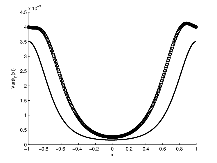
Both estimates and are random variables, depending on the random data observed, but we should hope that gives us a better approximation of , since it makes use of the true covariance (41). Indeed for simple linear statistical models, it is easy to see that an efficient estimator, which realizes the theoretically optimal variance given by the Cramér-Rao lower bound, may be obtained by using the true covariance of the data; however, using the incorrect covariance may lead to an estimate with significantly higher variance than the theoretical optimum. See [21] for more discussion of this point. The present setting is highly nonlinear and the variance of the estimates and cannot be computed explicitly, since depends on in a nonlinear way through solution of the PDE. Nevertheless the numerical results are consistent with the expectation that approximation of the true covariance (through homogenization theory) yields a MAP estimator that has smaller variance, relative to the estimate that makes no use of the homogenization theory (see Figure 3).

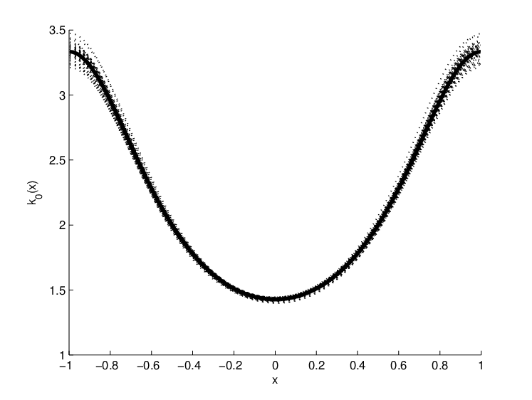
In Figure 1 we show one realization of the true coefficient which was used to generate the data. The highly-oscillatory graph represents the true coefficient with variation on many scales. The slowly-varying harmonic mean also is displayed here as the thick curve; this function is what we attempt to estimate. The data was generated as follows. Using one realization of and given forcing , we solve the Dirichlet boundary value problem (35). The observation data involves point-wise evaluation of at points spaced uniformly across the domain, plus independent observation noise at each point of observation. Using this data, we compute estimates and by minimizing (42) and (43), respectively. For the computation shown here, the function is parameterized by the first three coefficients in a Fourier series expansion. So, computing and involves an optimization in . To evaluate at each step in the minimization algorithm, we must solve the forward problem (40) with the current estimate of , and in the case of we must also compute . See [21] for more details about this computation.
Figure 2 compares the estimate with the true function . Since the estimate is a random function, we performed the experiment many times (generating new to compute each estimate ) and display the results of 100 experiments. The data for is qualitatively similar. Nevertheless, the pointwise variance is smaller than , as shown in Figure 3. This is consistent with the linear estimation theory for which knowledge of the true data covariance yields an estimate with optimal variance.
Acknowledgements.
The authors thank A. Cliffe and Ch. Schwab for helpful discussions concerning the groundwater flow model.Appendix 1
In this Appendix we prove Theorem 2.3 which, recall, applies in the case where (7b) and (13b) are replaced by periodic conditions on .
Theorem 5.1
Proof.
To simplify the notation we will set the porosity of the rock to be equal to , . Recall that Our first observation is that, for given by (9),
| (44) |
where
| (45) |
From Assumption 2.2 we deduce that
From the definition of it follows that
where
| (46) |
From the definition of in (14) we see that
Putting (44) and (46) together we see that
and we see from (45) and (46) that the perturbations of from are small; it is thus natural to expect a limit theorem for solving (8) which is Lagrangian transport in an appropriately averaged version of Furthermore, since is divergence free in the fast coordinate, by (15), it is natural to expect that the appropriate average is Lebesgue measure. We now demonstrate that this is indeed the case.
From (8) we deduce that
| (47) |
Define now and consider the system of SDEs
| (48a) | |||
| (48b) |
Since we see that , the solution of (48) is equal to appearing in (47).
The process is Markov with generator
Consider now the Poisson equation
| (49) |
with (see (13)(c))
Equation (49) is posed on with periodic boundary conditions. Notice that enters merely as a parameter in this equation. The operator is uniformly elliptic on and the right hand side averages to , hence, by Fredholm’s alternative this equation has a solution which is unique, up to constants. We fix this constant by requiring that . We define and similarly for . Applying Itô’s formula to and evaluating at we obtain
Consequently,
where
Since is periodic in both coordinates we have that
and
| (50) |
We combine the above calculations to obtain
where
and
Our estimates imply that
Furthermore, estimate (50), together with the Burkhölder-Davis-Gundy inequality imply that
On the other hand,
Set . Because is periodic it is in fact globally Lipschitz so that we obtain
where
We use Gronwall’s inequality to deduce
from which the claim follows. ∎∎
Appendix 2
In this appendix we study the homogenization problem (7) in one dimension. In this case we can calculate the homogenized coefficient explicitly and to prove Assumption 2.2. More details can be found in (24, Ch. 12).
The Homogenized Equations
We take in (7) and set Then the Dirichlet problem (7) reduces to a two–point boundary value problem:
| (51a) | |||||
| (51b) | |||||
We assume that is smooth in both of its arguments and periodic in with period 1. Furthermore, we assume that this function is bounded from above and below. Consequently, there exist constants such that
| (52) |
We also assume that is smooth.
The cell problem becomes a boundary value problem for an ordinary differential equation with periodic boundary conditions. Introducing the notation , the cell problem can be written as
| (53a) | |||
| (53b) |
Notice that the macrovariable enters the cell problem (53b) as a parameter. Since we only have one effective coefficient which is given by the one dimensional version of (11),(12), namely
| (54) | |||||
where we have introduced the notation . The homogenized equation is then
| (55a) | |||||
| (55b) | |||||
Explicit Solution of the Cell Problem
Equation (53a) can be solved exactly. After integrating the equation and applying the periodic boundary conditions, we obtain
with
Therefore, from (54) we obtain:
| (56) |
The constant is irrelevant. This is the formula which gives the homogenized coefficient in one dimension. It shows clearly that, even in this simple one–dimensional setting, the homogenized coefficient is not found by simply averaging the unhomogenized coefficients over a period of the microstructure. Rather, the homogenized coefficient is the harmonic average of the unhomogenized coefficient. It is quite easy to show that is bounded from above by the average of . Notice that the homogenized coefficient can be written in the form
| (57) |
Error Estimates in
The fact that we can obtain an explicit formula for the solution of the boundary value problem (51) as well as for the solution of the cell problem (53b) enables us to prove Assumption 2.2.
Proposition 5.2
Notice that, by (14), the corrector Hence, using the bound (52) from below on , together with the definition (9) of , this theorem delivers the following immediate corollary:
Corollary 2
Under the assumptions of Proposition 5.2 we have
Proof of Proposition 5.2. We have that
Consequently
Define a function by We solve the homogenized equation to obtain
with
Similarly, from (51) we obtain
with
From the above calculations we deduce that
It suffices to show that This will follow from the fact that
for any smooth function , as . To see this, define integer and uniquely by the identity
| (59) |
Then note that, using the uniform bounds on from below, together with uniform (in ) Lipschitz properties of and , we have for ,
This completes the proof. ∎
References
- (1) G. Allaire. Homogenization and two-scale convergence. SIAM J. Math. Anal., 23(6):1482–1518, 1992.
- (2) M. Avellaneda and F.-H. Lin. Compactness methods in the theory of homogenization. Comm. Pure Appl. Math., 40(6):803–847, 1987.
- (3) G. Bal, J. Garnier, S. Motsch, and V. Perrier. Random integrals and correctors in homogenization. Asymptotic Analysis, 59:1–26, 2008.
- (4) G. Bal and K. Ren. Physics-based models for measurement correlations: application to an inverse sturm-liouville problem. Inverse Problems, 25:055006, 2009.
- (5) H.T. Banks and K. Kunisch. Estimation Techniqiues for Distributed Parameter Systems. Birkhäuser, 1989.
- (6) A. Bensoussan, J.-L. Lions, and G. Papanicolaou. Asymptotic Analysis for Periodic Structures, volume 5 of Studies in Mathematics and its Applications. North-Holland Publishing Co., Amsterdam, 1978.
- (7) J.O. Berger. Statistical Decision Theory and Bayesian Analysis. Springer, 1980.
- (8) P.J. Bickel and K.A. Doksum. Mathematical Statistics. Prentice-Hall, 2001.
- (9) V.I. Bogachev. Gaussian Meausures. American Mathematical Society, 1998.
- (10) D. Cioranescu and P. Donato. An Introduction to Homogenization. Oxford University Press, New York, 1999.
- (11) S.L. Cotter, M. Dashti, J.C. Robinson, and A.M. Stuart. Bayesian inverse problems for functions and applications to fluid mechanics. Inverse Problems, 25:115008, 2009.
- (12) B. Dacarogna. Direct Methods in the Calculus of Variations. Springer, New York, 1989.
- (13) G. DaPrato and J. Zabczyk. Stochastic Equations in Infinite Dimensions. Cambridge University Press, 1992.
- (14) M. Dashti and A.M. Stuart. In preparation, 2010.
- (15) Y. R. Efendiev, Th. Y. Hou, and X.-H. Wu. Convergence of a nonconforming multiscale finite element method. SIAM J. Numer. Anal., 37(3):888–910 (electronic), 2000.
- (16) H.K. Engl, M. Hanke, and A. Neubauer. Regularization of Inverse Problems. Kluwer, 1996.
- (17) B. Fitzpatrick. Bayesian analysis in inverse problems. Inverse Problems, 7:675–702, 1991.
- (18) M. Hinze, R. Pinnau, M. Ulbrich, and S. Ulbirch. Optimization with PDE Constraints, volume 23 of Mathematics Modelling: Theory and Applications. Springer, 2009.
- (19) H. König. Eigenvalue Distribution of Compact Operators. Birkhäuser Verlag, Basel, 1986.
- (20) M.A. Lifshits. Gaussian Random Functions, volume 322 of Mathematics and its Applications. Kluwer, Dordrecht, 1995.
- (21) J. Nolen and G. Papanicoulaou. Inverse problems. Fine scale unertainty in parameter estimation for elliptic equations, 25:115021, 2009.
- (22) J. Nolen, G.A. Pavliotis, and A.M. Stuart. In preparation, 2010.
- (23) A. Papavasiliou, G.A. Pavliotis, and A.M Stuart. Maximum likelihood estimation for multiscale diffusions. Stoch. Proc. and Applics., 2009.
- (24) G. A. Pavliotis and A. M. Stuart. Multiscale Methods, volume 53 of Texts in Applied Mathematics. Springer, 2008. Averaging and Homogenization.
- (25) G.A. Pavliotis and A.M Stuart. Parameter estimation for multiscale diffusions. J. Stat. Phys., 127(4):741–781, 2007.
- (26) A.M. Stuart. Inverse problems: a Bayesian perspective. Acta Numerica, 19, 2010.