Fokker-Planck Asymptotics for Traffic Flow Models
Abstract.
Starting from microscopic interaction rules we derive kinetic models of Fokker–Planck type for vehicular traffic flow. The derivation is based on taking a suitable asymptotic limit of the corresponding Boltzmann model. As particular cases, the derived models comprise existing models. New Fokker–Planck models are also given and their differences to existing models are highlighted. Finally, we report on numerical experiments.
Key words and phrases:
Traffic Flow Modeling, Fokker–Planck Equations1991 Mathematics Subject Classification
Primary: 90B20; Secondary: 35L65Michael Herty
RWTH Aachen University
D-52056 Aachen, Germany
Lorenzo Pareschi
Department of Mathematics & CMCS, University of Ferrara
I-44100 Ferrara, Italy
November 19, 2009
1. Introduction
Kinetic models for traffic flow provide a description of vehicular traffic based on spatial, temporal and velocity information and have been subject to intense discussion in recent literature, see e.g., [5, 7, 8, 9, 10] and [11, 12]. In this paper we contribute to this discussion in the following way: we introduce microscopic interaction rules and derive existing and new equations using formal asymptotics and limits. This approach provides insight in the dominant terms of kinetic models and shows possible extensions.
Microscopic interaction rules yielding Boltzmann type traffic flow equations have been analyzed in [2]. Therein, the models by Klar et. al. [7, 8, 9, 10] could be derived from basic rules. However, the important class of Fokker–Planck type traffic flow models as introduced by Illner et. al. [11] could not be obtained. The present work now closes the remaining gap. We introduce general microscopic interaction rules as well as a derivation leading to the Fokker–Planck type models of Illner et. al. Further models corresponding to modified interaction rules are also discussed. In this work we do not want to discuss further the validity of such Fokker-Planck models (see [11] for a detailed discussion). We only remark that these models are particularly interesting from the computational viewpoint since they keep the kinetic information on vehicles without requiring the evaluation of the expensive velocity integrals as in Boltzmann-like models.
The main target is the single–lane, spatial homogenous Fokker–Planck type equations for traffic flow. The prototype example introduced ad–hoc in [11] is given by
| (1) |
where is the density of vehicles with velocity at time . Its motivation is as follows: is a heuristically defined braking and acceleration operator depending on moments of i.e., macroscopic quantities, like number density or mean velocity . They are defined as
The underlying assumption on both operators is that drivers only observe averaged quantities. The diffusive term is introduced to model the fact that drivers may not observe the averaged moments correctly. Furthermore, this operators allows for trivial equilibria corresponding to synchronized flow. Examples for the operators and are given in [11] and [3]
| (2) | |||
Herein are positive constants corresponding to braking and acceleration, is the indicator function. For convenience we normalize density and velocity such that The function ensures that the boundary conditions in the stationary case are met. It vanishes for large and small values of and . An explicit form can be found e.g. in [11]. It can be changed to , where is a residual diffusion to prevent discontinuous equilibria, see [3]. Furthermore, the function is motivated by additional lane–changing activity. It is modeled as
The coefficients and satisfy in order to obtain well-defined steady states.
In this paper, starting from microscopic considerations, we obtain a microscopic motivation for the given form of braking/acceleration and diffusion operators in the Fokker-Planck model. The microscopic rules will also lead to different but still qualitatively similar Fokker–Planck type models. Hence, in the sequel we start from a microscopic model with precise interaction rules between corresponding cars and derive on this grounds kinetic models of Boltzmann type. A suitable asymptotic limit then permits to recover the desired Fokker–Planck type models. We give the presentation for a general interaction of rule and state the corresponding equations for several well-known examples. Finally we report on numerical results for the different Fokker-Planck models.
2. Microscopic interaction rules and Boltzmann models
The interaction rules in traffic flow are different from the usual gas-dynamics case. In particular, traffic ”particles” are anisotropic, since a car that drives behind another one and speed up does not necessarily make the person in front go faster or slower. Additionally, acceleration and braking scenarios are not necessarily symmetric to each other.
We will present the derivation of the kinetic models for a general microscopic interaction rule. The leading car is assumed to have a pre–interaction velocity and a post–interaction velocity . We distinguish two different scenarios: if the leading car is slower than the one in front of it the leading car accelerates, cf. (3a). On the other hand, if it is faster it will decelerate or brake, cf. (3b). A simple model is as follows: we compare our velocity with the velocity of the car in front. If we are faster, we brake according to the relative velocity, if we are slower we accelerate. Since we cannot precisely estimate the leading car’s velocity and we will made mistakes when braking and accelerating. The modeling includes therefore some additional parameters and a noise term proportional to braking and acceleration intensity characterized by a random variable .
The general form of the microscopic interaction rule is
| (3a) | |||
| (3b) | |||
where represents the estimate on the leading car velocity made by the driver. The coefficients , represent the desired velocities when drivers accelerate and brake. Thus the natural choice is with a monotone non decreasing function of . Beside the obvious choice other choices for , although less realistic, are interesting since they lead to simplified set of equations. For example where drivers are able to estimate only the mean velocity of the flux. Similarly and may depend on the actual velocity and the estimated relative velocity .
To complete the interaction we leave the velocity of of the car in front unchanged, i.e.,
In (3) and are non negative constants in , is a power that calibrates the dependence of the noise from the braking/acceleration dynamic, is a function that takes into account that noise is also proportional to the actual driver speed and is a random variable with zero mean and variance distributed accordingly to .
The above microscopic relations include as particular cases several well-known models. We give some examples.
- •
Example 1: The model by Illner, Klar & al. [6]. In this model we assume that individual estimates correctly the leading car’s velocity and that acceleration and braking are bounded by the maximal and minimal velocity instead of the velocity of the leading car
- •
Example 2: A generalized model by Günther, Klar & al.[4]. Drivers interact via symmetric braking and acceleration scenarios governed by the leading car and can estimate correctly the leading car velocity
Note that in the original model no diffusion was present .
- •
Example 3: If we assume that individuals react with respect to the average velocity and that acceleration and braking are bounded by the average velocity we have the set of parameters
This model as we will see permits to derive the Fokker-Planck equation (2) from the microscopic dynamics in a suitable asymptotic scaling.
Some remarks are in order.
Remark 1.
- (1)
In the microscopic model it is possible to add a further term independent of the other drivers behavior
(4) From a modeling point of view this corresponds to free flow traffic adjusting towards a certain desired velocity distribution To keep the derivation simple we will ignore the presence of this free flow term in the sequel.
- (2)
Note that in (3) we require that the post-interaction velocities satisfy . We can show that this is guaranteed by our assumptions on the parameters. Let us show this for the acceleration term. Since we have
if . Note that for close to the domain of vanishes. One can show that independently of we have if . However in the sequel we will be interested in the behavior of the model for small values of and and for such reason we will take simply .
It is easy to see that if . Note however that in this case for small values of the domain of vanishes. If we assume that we get
if which permits to pass to the limit keeping finite.
Similarly for the braking term we have provided that and . Thus if we want to preserve the lateral bounds of . To this end the presence of the function is of importance. is such that it vanishes at the extreme values of the velocity and . This can be achieved by any function such that for . For example we might take
or a quadratic function like
This implies that the diffusion term in (3a)-(3b) vanishes in correspondence of the desired speeds and at the extremal values and of the velocity domain.
As mentioned in the introduction a general Boltzmann–type formulation for vehicular traffic was derived in [2]. For simplicity we restrict to the case in (3) we will come back to other choices at the end of the next section.
In weak form we can write for the car distribution the kinetic equation
| (5) |
where
| (6a) | |||||
| (6b) | |||||
Additionally, as in [2] we assume that the function is given by
where is the indicator function. In the general case (3) the collision kernel has a weight of .
From (6a)-(6b) conservation of the total number of vehicles is obtained for which represents the only conservation property satisfied by the equation. If we consider the case (this corresponds to the behavior of the mean velocity) we obtain
Hereby we assume that the random variables in the acceleration and the braking terms take values on the sets and respectively. Now the second and the fourth integrals vanish since has zero mean and so we have
which represents the change in mean velocity due to acceleration and braking.
If we assume and we can write
In Example 2 we have . In this case a straightforward computation shows that the mean velocity is conserved. This situation has much in common with a granular gas dynamic where is related to the coefficient of restitution, and the large time behavior of the system in absence of diffusion () is described by synchronized traffic given by a Dirac delta where all cars have the same speed . Note that the synchronized traffic state is an equilibrium state of the system even in the general case when and since the noise term vanishes when all cars have the same speed.
One of the major drawbacks of Boltzmann-type models is their excessive complexity which makes it difficult the development of numerical simulation methods as well of analytical tools for the computation of steady states.
In order to obtain simpler kinetic Fokker–Planck type equations we use a suitable asymptotic limit similar to the technique presented in [13]. In the latter presentation only a global and symmetric interaction rules for a Maxwellian-like kernel have been considered. Other similar interaction rules in the context of opinion formation has been studied in [14]. We emphasize that in the following, the interaction is anisotropic and the collision kernel is of hard-spheres type. Therefore it is different to [13, 14] and also to standard approaches in gas–dynamics.
3. Fokker–Planck type asymptotic models
First let us recall some definitions. We define the space of all probability measures in and by
| (8) |
the space of all Borel probability measures of finite momentum of order , equipped with the topology of the weak convergence of the measures. Let , be the class of all real functions on such that , and is Hölder continuous of order ,
the integer and the number are such that , and denotes the -th derivative of .
In the rest of the paper we will assume that the symmetric probability density which characterizes the transition rate belongs to , for some . Moreover, to simplify computations, we assume that this density is obtained from a given random variable with zero mean and unit variance, that belongs to . Thus, of variance is the density of . By this assumption, we can easily obtain the dependence on of the moments of . In fact, for any such that the -th moment of exists,
To skip inessential difficulties, that do not change the following analysis, we suppose that the random variables in the acceleration and the braking terms take values on the sets and respectively. We also assume that for .
In order to derive a Fokker–Planck equation from (6) we need to consider an appropriate scaling of the equations. We set for
| (9) |
and assume that there exists non–negative constants and with the following properties
| (10) |
These assumptions corresponds to an asymptotic situation where each interaction produces very small velocity variations and in the limit we preserve the main features (deterministic acceleration/braking and random noise) of the dynamic.
The scaled kinetic equation reads
| (11) |
For small values of and we have and so we can consider a Taylor expansion in the collision kernels and of around Let us consider here the acceleration term (3a)
where for some we have
Now we insert this expansion into the acceleration operator and compute the limit for Since has mean zero and vanishing variance we get
where
Since , and
| (12) |
Hence
By virtue of the inequality
and using the fact that is compactly supported in we finally obtain the bound
| (13) |
Since is a probability density with zero mean and variance, and belongs to , for ,
and is bounded. Using this equality one shows that converges to zero as .
Thus we obtain
By similar arguments for we get
In order to present the strong formulation of the limiting kinetic equation we introduce the following constants
| (14) |
Summarizing, the above computations we observe that in the limit we obtain the following Fokker–Planck equation given in strong form by
| (15) | |||
which can be rewritten in more compact notation as
| (16) | |||
| (17) | |||
where
Furthermore, it is useful to introduce the partial moments for fast and slow cars as follows
In this way we can rewrite the limiting Fokker-Planck equation in the form
| (18) |
For the interaction rules presented in the previous section we have the following equations in the limit
- •
Example 1: For the model by Illner, Klar & al. we get
(19) or using the partial moments
- •
Example 2: For the generalized model by Günther, Klar & al. we obtain
(20) - •
Example 3: For the model where individuals react with respect to the average velocity we have
(21a) (21b)
Remark 2.
- •
The evaluation of the partial moments which appears in examples 1 and 2 can be done efficiently at a numerical level at the same computational cost of the computation of mass and momentum. This is of paramount importance in applications of the the Fokker-Planck models to realistic simulations.
- •
The general Fokker-Planck equation (15) derived above preserve the essential properties of the microscopic relations it came from. For example mean velocity is preserved only when and . Similarly synchronized traffic is a possible equilibrium state of the system when . Moreover upper and lower bounds for the cars velocities are satisfied thanks to the presence of .
4. Relations with Illner, Klar, Materne model
We analyze some of the derived models and compare them to Illner, Klar, Materne model.
Let us at first consider Example 3 and assume that is independent of and set
i.e., .
We can differentiate in the diffusion term and obtain
By comparing this equation with the original model by Illner et. al. (2) we observe the following. Since we did not include lane changing in the microscopic interaction rules we can only compare with (2) in the case The previous derivations hold true also in the case when the quantities and are and dependent. Hence, if they are chosen such that
| (22) |
we exactly recover the model by lllner et. al. (2) for In the cases we can recover the exponent in the diffusion but obtain additional drift terms to a power of We also observe that we immediately obtain the lower bound on for positive
Moreover the diffusion term is degenerate when . Adding a modified diffusion such as will off course remove the degeneracy but destroys the possibility of synchronized traffic as discussed in [3].
Let us now consider Example 2. We approximate the partial moments in (20) close to synchronized traffic
At synchronized traffic the operators and collapse to
and under the additional assumption and using the same choices for the constants and as before, we again obtain (2) in the case . Therefore, the model (20) can be seen as a generalized equation comprising (2) and at the same time linking the coefficients appearing in diffusion and braking terms to microscopic interaction rules.
Note however that in the computation reported above to connect our Fokker-Planck models with Illner & al. model we assumed that is constant. Thus there is no mechanism to prevent the solution to violate the lateral bounds for the car velocity.
We discuss some particular cases. The limit case in Illner’s model for the diffusion coefficient is which implies in the microscopic rules (3). This implies a constant diffusion in the microscopic interaction rules (3). This seems at least questionable. On the other hand taking corresponds to being the upper limit case for Illner’ s model. In this case the noise is directly proportional to the difference in the velocities.
Finally, we compare the diffusion terms of (2), i.e.,
and (20) in the case , i.e.,
We observe, that the Fokker–Planck derived from microscopic rules has a convolution integral in the diffusion term compared to the degenerated diffusion in the Illner model. Hence, in the steady states we expect a smoother distribution profile Furthermore, the degeneracy at is not present in the second case. This is a remarkable feature of (20) with respect to (2).
5. Steady states and numerical experiments
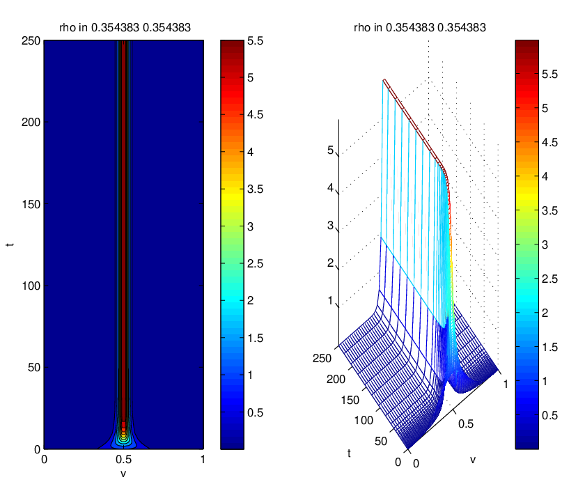
In this section we report on numerical results for the models (19), (20) and (21). In all models we set the cut–off in the diffusive part as and hereby normalize the computational domain for to We use discretization points on for all computations. We apply the methods of lines with a time horizon of . The large time horizon is chosen in order to capture the steady state solution. When discretizing in we use a simple first–order upwind discretization for the first–order derivatives and centered differences for the diffusion term. The final system of ordinary differential equations is then solved by an implicit Euler method. During simulations the total mass is preserved. The initial data for the simulation is chosen such that it vanishes at the boundary and given by The initial mass is For simplicity we set in all simulations.
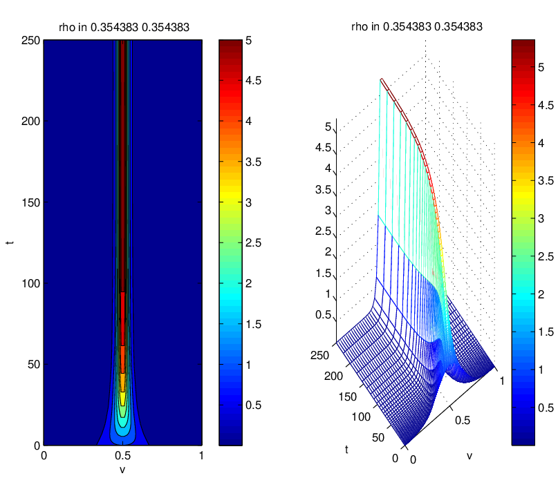
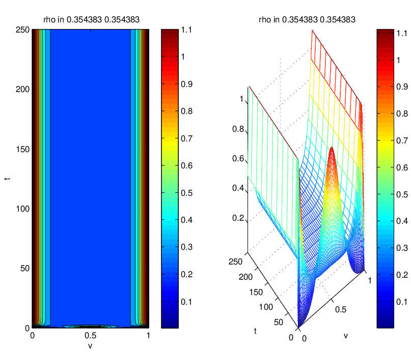
At first we study the dependence of the time evolution of on the diffusion coefficient if the dynamics is controlled by example 1 (19), i.e.,
The braking and acceleration constants are . We present plots of the isolines of the solution as well as a three–dimensional for diffusion coefficients between and in figure 1. We observe a concentration forming from the initial Gaussian curve. As we increase the diffusion parameter the center of the concentration moves from to the boundaries . A similar behavior is observed when simulating example 2, (20), i.e.,
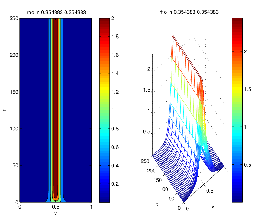
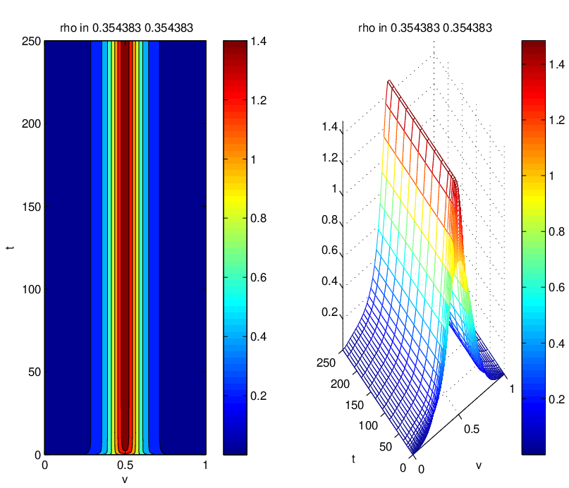
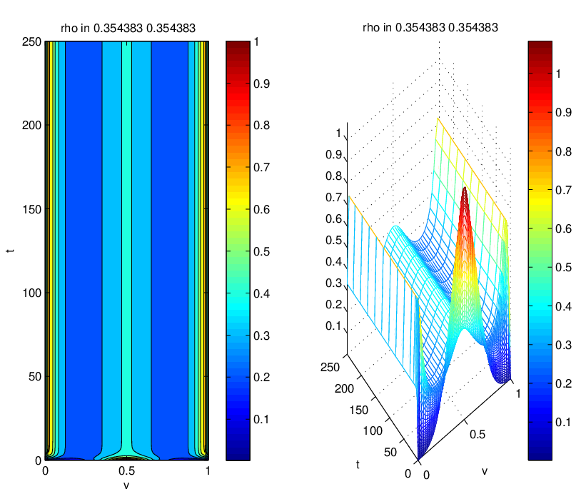
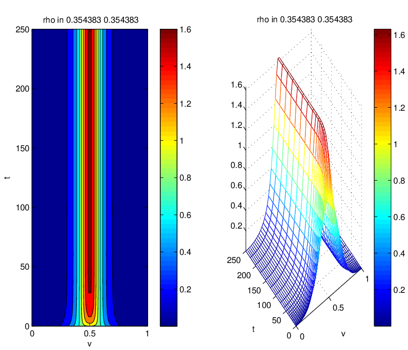
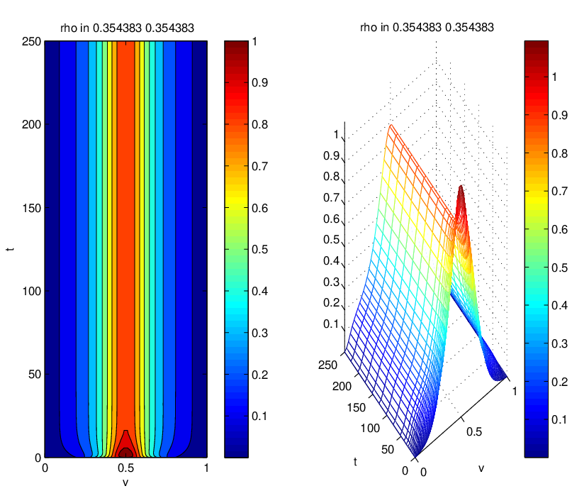
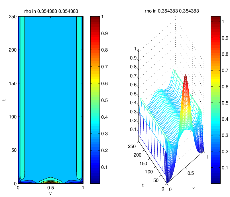
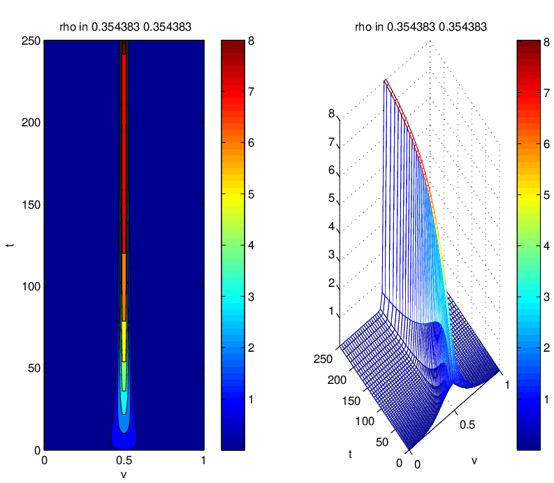
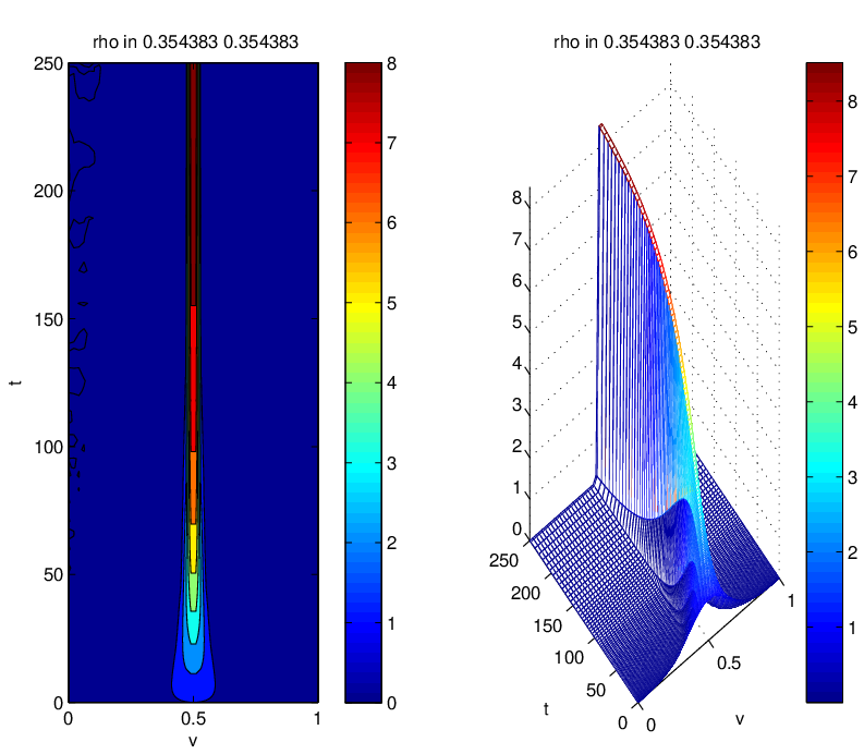
Using the same parameters and setting we observe in figure 2 the same qualitative behavior. For small diffusion coefficients we observe a concentration at the center and for larger coefficients at the boundary and . Next, we study the dependence of the time evolution on the other parameters present in example 2. In figure 3 we observe that the exponent in (20) does not influence the qualitative behavior. We give a result for a moderate diffusion parameter and the case and However, the braking and acceleration constants have a strong influence on the position of the concentration. In the case and and we observe a shift of the point of concentration away from . Clearly, the obvious interpretation is: if the braking force is stronger than the acceleration force the equilibrium distribution must concentrate in a regime of lower velocity. The results are given in figure 4 and has to be compared with the corresponding part in the upper left of figure 1 where we used


Concerning Example 3, (21), a comparison between the derived model and the original model of Illner et. al. is given. Here, we compare the long term behavior in terms of the arising steady state. In case of Illner’s model (2) these can be computed explicitly [3] and are given by
| (23) |
Here, it is assumed that . The constants are such that mass and momentum equation are satisfied, i.e., In case of Example 3 we also compute the steady states as
Again, the constants are such that The additional factor in the steady state is due to the fact that the diffusion is now velocity dependent. If the following relations hold true, both steady states coincide:
| (24) |
6. Conclusions
Starting from microscopic vehicles interactions we derived Fokker-Planck models for traffic flows as a suitable asymptotic limit of a Boltzmann dynamic. Among others the new Fokker-Planck models include the model recently introduced by Illner al. [2]. A remarkable feature of these models is to preserve synchronized traffic states and to avoid the degeneracy in the diffusion term when the vehicle velocity coincides with the mean velocity. These kinetic models are very promising for numerical simulation purposes since their computational cost is strongly reduced when compared to full Boltzmann models. Numerical results for the non homogeneous multilane case are under progress and will be presented elsewhere.
Acknowledgements
This work has been supported by DAAD D/06/19582, DFG HE5386/6-1, HE5386/8-1, RWTH Seed Funds and Vigoni Project “Numerical methods for the simulation and the optimization of traffic flows on networks”. The first author would like to thank University of Ferrara for their hospitality.
References
- [1] S. Cordier, L. Pareschi and G. Toscani. On a Kinetic Model for a Simple Market Economy. Journal of Stat. Phys., 120, (2005), pp. 253–277.
- [2] M. Herty, A. Klar and L. Pareschi. General kinetic models for vehicular traffic flow and Monte Carlo methods. Comput. Methods Appl. Math., 5, (2005), pp.155–169.
- [3] M. Herty, R. Illner, A. Klar and V. Panferov. Qualitative Properties of Solutions to Systems of Fokker-Planck equations for Multilane Traffic Flow. Transp. Theo. Stat. Phys., 35, (2006), pp. 31–54.
- [4] M. Günther, A. Klar, T. Materne, and R. Wegener. An explicitly solvable kinetic model for vehicular traffic and associated macroscopic equations, Math. Comp. Model., 35 (2002), p. 591.
- [5] D. Helbing. Gas-kinetic derivation of Navier-Stokes-like traffic equations. Phys. Rev. E 53 (1996), pp.2366–2381.
- [6] R. Illner, A. Klar, H. Lange, A. Unterreiter, and R. Wegener. A kinetic model for vehicular traffic: Existence of stationary solutions, J. Math. Anal. Appl., (1999).
- [7] A. Klar and R. Wegener. Enskog-like kinetic models for vehicular traffic, J. Stat. Phys., 87 (1997), pp. 91–114.
- [8] A. Klar and R. Wegener. A hierachy of models for multilane vehicular traffic I: Modeling, SIAM J. Appl. Math., 59 (1998), pp. 983–1001.
- [9] A. Klar and R. Wegener. A hierachy of models for multilane vehicular traffic II: Numerical investigations, SIAM J. Appl. Math., 59 (1998), pp. 1002–1011.
- [10] A. Klar and R. Wegener. Kinetic derivation of macroscopic anticipation models for vehicular traffic, SIAM J. Appl. Math., 60 (2000), pp. 1749–1766.
- [11] R. Illner, A. Klar and T. Materne. Vlasov–Fokker–Planck models for multilane traffic flow. Comm. Math. Sci., Vol 1, 2003, pp. 1–12
- [12] R. Illner, C. Stoica, A. Klar and R. Wegener. Kinetic equilibria in traffic flow models. Transp. Theo. Stat. Phys. 31, (2002), pp. 615–634.
- [13] L. Pareschi and G. Toscani. Self–Similarity and Power–Like Tails in Nonconservative Kinetic Models. Journal of Stat. Phys., Vol 124(2–4), pp. 747–779, 2006.
- [14] G. Toscani. Kinetic models of opinion formation. Commun. Math. Sci., Volume 4, Number 3 (2006), pp.481-496.
Received xxxx 20xx; revised xxxx 20xx.