Continuum simulations of shocks and patterns in vertically oscillated granular layers
Abstract
We study interactions between shocks and standing-wave patterns in vertically oscillated layers of granular media using three-dimensional, time-dependent numerical solutions of continuum equations to Navier-Stokes order. We simulate a layer of grains atop a plate that oscillates sinusoidally in the direction of gravity. Standing waves form stripe patterns when the accelerational amplitude of the plate’s oscillation exceeds a critical value. Shocks also form with each collision between the layer and the plate; we show that pressure gradients formed by these shocks cause the flow to reverse direction within the layer. This reversal leads to an oscillatory state of the pattern that is subharmonic with respect to the plate’s oscillation. Finally, we study the relationship between shocks and patterns in layers oscillated at various frequencies and show that the pattern wavelength increases monotonically as the shock strength increases.
pacs
45.70.-n, 45.70.Qj, 47.40.Nm, 47.54.-rI Introduction
I.1 Background
Vertically oscillated granular layers provide an important testbed for granular research. When shaken vertically, flat layers of grains exhibit convection [1], clustering [2], shocks [3], steady-state flow fields far from the plate [4], floating particle clusters [5], and standing-wave pattern formation [6].
In this paper, we model granular media by numerically solving a set of time-dependent continuum equations for the rapid flow of dissipative particles in three-dimensions. We use these simulations to investigate the relationship between shocks and standing-wave patterns in vertically oscillated granular layers.
I.2 Granular hydrodynamics
A successful theory of granular hydrodynamics would allow scientists and engineers to apply the powerful methods of fluid dynamics to granular flow. Despite experimental [7, 9, 8] and computational [10, 11, 12, 13, 8] evidence demonstrating the potential utility of hydrodynamics models for grains, a general set of hydrodynamic governing equations is not yet recognized for granular media [14, 15, 16, 17].
Several proposed rapid granular flow models use equations of motion for continuum fields: number density , velocity , and granular temperature ( is the average kinetic energy due to random particle motion) [18, 19, 20]. In one approach, particle interactions are modeled with binary, inelastic hard-sphere collision operators in kinetic theory to derive continuum equations to Euler [21], Navier-Stokes [22], and Burnett [23] order. We use three-dimensional (3D) simulations of continuum equations to Navier-Stokes order to investigate shocks and standing-wave patterns in shaken granular layers.
I.3 Standing wave patterns in oscillated granular layers
A granular layer of depth atop a plate that is oscillated sinusoidally in the direction of gravity with frequency and amplitude will leave the plate at some time during the oscillation cycle if the maximum acceleration of the plate is greater than the acceleration of gravity . In other words, the layer leaves the plate if the nondimensional accelerational amplitude exceeds unity.
After leaving the plate, the layer dilates above the plate, and then compresses when it collides with the plate later in the cycle. When the dimensionless accelerational amplitude is larger than a critical value , standing-wave patterns spontaneously form in the layer. These patterns are subharmonic with respect to the plate, repeating every [6]. Depending on the nondimensional accelerational amplitude and dimensionless frequency , various subharmonic standing waves have been found, including stripe, square, and hexagonal standing-wave patterns [6].
I.4 Shocks in oscillated granular layers
If the Mach number (the ratio of the local mean fluid speed to the local speed of sound) is greater than unity at the point where a fluid encounters an obstacle, a compression wave front is formed near the object and steepens to form a shock. A distinguishing feature of granular materials is that granular flows reach supersonic speeds under common laboratory conditions [18, 9, 3]. Therefore, although shocks are formed in ordinary gases only under extreme conditions, shock formation is commonplace in granular media.
Experiments [3] and simulations [24, 25, 26, 11] demonstrate that shock waves form in shaken granular layers as the layer contacts the plate. Previous investigations have generally either focused on shock propagation [3, 24, 25] or pattern formation [6, 12, 13] or considered them as separate phenomena coexisting in shaken layers [11]. In this paper, we use continuum simulations to investigate the interactions between shocks and the standing-wave patterns formed in this system.
I.5 Model system
We simulate a layer of grains on an impenetrable plate which oscillates sinusoidally in the direction of gravity. The layer depth at rest is approximately where the grains are modeled as identical, frictionless spheres with diameter , mass , and coefficient of restitution . In this paper, we study patterns and shocks as a function of nondimensional frequency , while the dimensionless accelerational amplitude is held constant. Previous simulations [12, 13] have shown that this value exceeds the critical accelerational amplitude indicating that we should expect to see standing-wave patterns for a variety of frequencies.
Previous experiments [27] and molecular dynamics (MD) simulations [28] have shown that friction between grains plays a role in these patterns. Experimentally, adding graphite to reduce friction decreased and prevented the formation of stable square or hexagonal patterns found for certain ranges of and in experiments without graphite [27]. Similarly, MD simulations with friction between particles have quantitatively reproduced stripe, square, and hexagonal subharmonic standing waves seen experimentally [29], but MD simulations without friction yield only stable stripe patterns and display a lower [28]. In this study, we investigate stripe patterns in continuum simulations of frictionless particles. To investigate other patterns such as squares or hexagons, simulations would have to include friction between particles.
Experiments [30] and simulations [31, 12, 13] indicate that fluctuations due to individual grain movement play a larger role in granular media than do thermal fluctuations in ordinary fluids. Fluctuating hydrodynamics (FHD) theory models these fluctuations by adding noise terms to the Navier-Stokes equations [32, 33, 34]. In previous simulations with FHD noise terms, the critical value of pattern onset was consistent with molecular dynamics simulations, while continuum simulations without these fluctuations exhibited pattern onset at approximately lower than that found in MD simulations [12, 13]. Above , however, simulations both with and without these fluctuations exhibited standing-wave patterns with wavelengths consistent with a dispersion relation [35] found experimentally for a range of shaking frequencies. In this paper, we do not include FHD noise terms; we investigate patterns for accelerational amplitude greater than determined from simulations with and without FHD.
We use continuum simulations to investigate the dynamics of this system including pattern formation and shock propagation. Section II describes the methods we use to simulate and analyze oscillated layers. Sec. III examines the dynamics of shocks and standing-wave patterns formed in this system at a fixed dimensionless oscillation frequency , and Sec. IV examines how these patterns and shocks change when this frequency is varied. We present our conclusions in Sec. V.
II Methods
II.1 Continuum equations
We use a continuum simulation previously used to model shock waves in a granular shaker [26]. Our simulation numerically integrates continuum equations of Navier-Stokes order proposed by Jenkins and Richman [22] for a dense gas composed of frictionless (smooth), inelastic hard spheres.
This model yields hydrodynamic equations for number density (or equivalently, volume fraction ), velocity , and granular temperature :
| (1) |
| (2) |
| (3) |
where the components of the symmetrized velocity gradient tensor are given by: The components of the stress tensor are given by the constitutive relation
| (4) |
and the heat flux is calculated from Fourier’s law:
| (5) |
To calculate the pressure, we use the equation of state and radial distribution function at contact proposed by Goldshtein et al. [36] to include both dense gas and inelastic effects:
| (6) |
where
| (7) |
and the radial distribution function at contact, , is
| (8) |
where is the 3D random close-packed volume fraction.
These equations differ from those for a compressible, dense gas of elastic particles by the energy loss term
| (9) |
which arises from the inelasticity of collisions between particles. The bulk viscosity is given by
| (10) |
the shear viscosity by
| (11) |
and the thermal conductivity by
| (12) |
Other hydrodynamic models include modifications such as more accurate expressions for kinetic coefficients which incorporate high density corrections [37, 38] and equations of state which allow for volume fractions greater than the random-close-packed limit used here [39]. However, the equations shown here have previously been used to separately examine shocks [26] and patterns [12, 13] in shaken layers and have demonstrated quantitative agreement with experiments and molecular dynamics simulations. Therefore, we use these equations in this study to investigate the relationship between shocks and pattern formation; in principle, the equations could be modified to implement other forms of the constitutive relations.
II.2 Simulation method
We integrate these hydrodynamic equations to find number density, momentum, and granular temperature, using a second order finite difference scheme on a uniform grid in 3D with first order adaptive time stepping [26]. In these simulations, the granular fluid is contained between two impenetrable horizontal plates at the top and bottom of the container, where the lower plate oscillates sinusoidally between height and and the ceiling is located at a height above the lower plate. Periodic boundary conditions are used in the horizontal directions and to eliminate sidewall effects. Simulations were conducted in a box of size , , and . This orientation causes stripes to form parallel to the -axis. The numerical methods, boundary conditions at the top and bottom plate, and grid spacing are the same as used in previous studies of shocks [26] and patterns [12, 13].
III Dynamics of Shocks and Standing Waves
III.1 Standing wave patterns
Experimental investigations of shaken granular layers have shown that above a critical acceleration of the plate , standing wave patterns form spontaneously. These patterns oscillate subharmonically, repeating every , so that the location of a peak of the pattern becomes a valley after one cycle of the plate, and vice versa [6].
Continuum simulations produce standing wave patterns for and (Fig. 1). Beginning with a flat layer above the plate with small amplitude random fluctuations, the simulation ran for 250 cycles of the plate until the layer reached a periodic state. Snapshots from various times during the next two cycles of the plate are shown in Fig. 1. Alternating peaks and valleys form a stripe pattern which oscillates at with respect to the plate oscillation; a location in the cell which represents a peak during one cycle will become a valley the next cycle, and then return to a peak on the following cycle. We examine the wave patterns at various times in the cycle for two cycles of the plate.
Volume Fraction


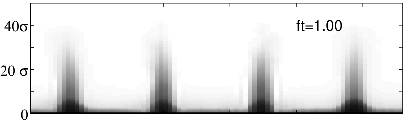


III.1.1 : The layer collides with the plate.
At the container is at its minimum height. The bulk of the layer is dilute and four clear peaks and four valleys are evident in Fig. 1 (note that one of the peaks wraps around the edges of the cell since the boundary conditions are periodic). The material in each peak is falling towards the plate, although the bottom of the layer has begun to contact the plate and is beginning to form a pile on the plate. The thin layer colliding with the plate is characterized by a higher volume fraction than the material in the peaks.
III.1.2 : The layer piles on the plate.
At , the plate has begun move upward as the layer falls to meet it. At this time, most of the layer is piling on the plate, forming a high volume fraction region near the plate. Remnants of the peaks and valleys from the previous cycle are still visible, although the layer is flattening on the plate, with the height difference between peaks and valleys much smaller than at (Fig. 1).
III.1.3 : The layer begins to leave the plate.
As the container reaches its maximum downward acceleration at the top of its oscillation, the layer begins to leave the plate. Although the bottom of the layer is still in contact with the plate at this time, the layer is expanding, as evidenced by the fact that it is visibly more dilute in this picture than in the previous snapshot (Fig. 1). As the layer leaves the plate, new peaks and valleys develop, with peaks forming in the valleys from the previous cycle, and vice versa.
III.1.4 : The layer is off the plate.
At , the plate is moving downward leaving a gap between the layer and the plate. The mass of the layer has almost entirely left the plate, and the layer has expanded. The new peaks and valleys have become quite distinct, with a large portion of the layer in the peaks and very little material in the valleys connecting them (Fig. 1).
III.1.5 : The cycle repeats.
At , the plate has undergone one full oscillation and has returned to its lowest point in the cycle. The features of this point in the cycle are similar to those at , except the peaks and valleys have reversed location. Aside from the peaks and valleys reversing, the next cycle exhibits the same features as the previous cycle at all times during the cycle. By the peaks and valleys are back to their original location, demonstrating the subharmonic nature of these patterns.
III.2 Shocks
Previous experiments [3] and simulations [24, 25, 26, 11] indicate that shocks are formed in vertically oscillated granular layers during each collision of the layer with the plate. A prerequisite for shock formation is that the local Mach number of the flow be greater than unity with respect to the object causing the disturbance. Therefore, we calculate the speed of sound using a relation derived from the equation of state Eq. (6) [40]:
| (13) |
where . The Mach number is calculated as the local flow speed divided by the local speed of sound .
Horizontal Location
Horizontal Location


From Fig. 1, we see that at , a portion of the layer has begun to compress on the plate, while some of the material is still falling towards the plate. This is therefore a time at which we would expect to see shock formation. To examine the shock in detail, we plot one-dimensional profiles of volume fraction and Mach number (here is scaled by a factor of 10 to fit on the same scale as ) as functions of height from the plate in Fig. 2.
At , the first peak of the pattern occurs at the horizontal location (cf Fig. 1). We choose two horizontal locations to examine; the location , and is shown in the left column of Fig. 2, corresponding to the first peak of the pattern; the location , and is shown in the right column, corresponding to a location away from the peak.
At the horizontal location , corresponding to a peak of the wave pattern, the volume fraction approaches the close-packed value near the plate at (Fig. 2a). As height increases, smoothly decreases for . The Mach number with respect to the plate is low throughout this region, as this part of the layer is compressed on the plate and thus matches the velocity of the plate at height . However, at , there is a discontinuity in the derivative of , and a sharp increase in Mach number such that for . This sharp increase in Mach number from subsonic to supersonic, corresponding to a discontinuity in the derivative of volume fraction at the same height, indicates that this is the location of a strong shock front.
While the above description applies to (the horizontal location of the first peak), a shock also forms in the valleys. This can be seen in Fig. 2b, which shows and at the same time, but at horizontal location . Here we again see a high density, subsonic region near the plate, with a shock separating this region from a lower density, supersonic undisturbed region that is still falling towards the plate. However, the volume fraction near the plate is smaller than it was in Fig. 2a, and the shock profile is quite different. Also, the shock front at is closer to the plate than it is at .
By , the shock has moved away from the plate and it continues to develop as it moves through different parts of the layer (Fig. 2c). The shock front in the valleys is also developing and moving away from the plate (see Fig. 2d), although the location and profile of the shock is different at these different horizontal locations.
Thus, shocks form with each collision of the layer with the plate, and the shock profile changes and develops as the shock moves through the layer. Shocks form at each horizontal location in the cell; however the shock front is non-uniform horizontally due to the differences in layer depth between the peaks and the valleys of the pattern.
III.3 Interaction between shocks and patterns
There is therefore a relationship between the shocks and the standing-wave patterns formed in the layer. If the layer were perfectly flat, the shock front would be uniform horizontally. However, as there is horizontal variation in layer depth, a non-uniform shock front forms.
While the system is driven by vertical motion of the plate, the patterns are characterized by horizontal variation between peaks and valleys. Periodic horizontal motion is required to produce the subharmonic oscillation. This horizontal flow can be thought of as a “sloshing” motion, in which material from the layer flows out of some regions and into others, creating peaks and valleys. With the next collision of the layer with the plate, the flow direction reverses, creating peaks where there were valleys, and vice versa. In this section, we show that strong pressure gradients created by the shock drive the sloshing motion of the layer.
To study this interaction, we investigate the layer properties near the time of shock formation. According to Fig. 1, most of the layer is off the plate at , while the layer is compressed on the plate and the peaks and valleys have flattened significantly by . In Fig. 3 we show snapshots of the the volume fraction (left column) and the dimensionless pressure (right column) at five different times . We display side views of the layer at in (Fig 3), showing only the horizontal range and the vertical range to better view the interaction between the layer and the plate. This range shows two wavelengths of the standing wave pattern and corresponds to the bottom left quadrant of the range plotted in Fig. 1.
In order to examine the sloshing motion of the layer, we also show the dimensionless -component of the pressure gradient (left column) and the dimensionless horizontal velocity (right column) at the these same times and locations in Fig. 4. We now proceed to examine the horizontal variation in flow at these five times as the layer collides with the plate.
Volume Fraction
Dimensionless Pressure


Dimensionless Horizontal Pressure Gradient
Dimensionless Horizontal Velocity


III.3.1 The layer is off the plate.
At , the layer is mostly off the plate, and peaks and valleys are clearly visible in the left column of Fig. 3. In the right column of Fig. 3, we show the dimensionless pressure . At this time, the layer is more dilute than it will be at later times in the cycle, and the pressure is uniformly low throughout the layer. There are no strong pressure gradients visible, as can be seen in the left column of Fig. 4, where we show the dimensionless -component of the pressure gradient .
In the right column of Fig. 4, we can see that (the flow is moving towards the right) for ; there is a small range of nearly zero horizontal flow rate near ; then (flow is moving towards the left) for . Since the peak of the pattern is located at at this time (cf Fig. 3), grains are flowing towards the peak from both the left and the right. Therefore, the flow is still removing material from the valleys and moving it towards the peak; the difference between peaks and valleys is growing at this time.
III.3.2 The layer begins to contact the plate.
At , the bottom of the layer has just begun to contact the plate at the horizontal location of the two peaks, but the material between the peaks has not yet contacted the plate (Fig. 3). The layer looks similar to its appearance at , except that in a very small region near the plate, the pressure has begun to slightly increase where the layer is starting to contact the plate.
This pressure increase at the two points of contact yields a horizontal pressure gradient with maximum pressure near the peak location. For instance, the reddish color found near the plate for in the left column of Fig. 4 at this time indicates that the pressure is increasing from left to right; the bluish color for in the same picture indicates that the pressure decreases from left to right.
The picture in the right column for this time shows that the flow is still moving towards the peak through the bulk of the layer at this time. However, the pressure gradient near the plate tends to drive flow in the opposite direction: from high pressure (near the peak) into low pressure (near the valley). Therefore, the horizontal flow velocity near the plate has begun to slow (leaving a white space near the plate where the pressure gradient is strongest) and is even beginning to reverse direction (note the light blue near the plate at the location of the second peak).
III.3.3 A shock forms.
By , more of the material is colliding with the plate, and the pressure has noticeably increased at the two main contact points between the layer and the plate (Fig. 3). This increase in layer density and pressure near the plate marks the formation of a shock (cf Fig. 2).
As discussed in Sec. III.2, these shocks are not uniform horizontally; larger layer depth near the peaks leads to larger pressure at these locations. Thus, shock formation leads to pressure maxima near the plate at the horizontal location of the pattern peaks with strong pressure gradients as seen in the left column of Fig. 4.
These pressure gradients drive the flow in the direction opposite the pressure gradient; thus the direction of flow near the plate at this time is clearly reversing (see the right column of Fig. 4). For much of the layer, the flow is still away from the valleys and towards the peaks. Near the plate in the region of strong pressure gradients, however, the flow has reversed itself and is now flowing away from the peaks and towards the valleys. This separation of the flow into two distinct domains represents the formation of a shock near the plate.
III.3.4 The shock propagates.
This shock then travels upward through the layer, away from the plate. By , this shock is well-developed and has propagated through most of the layer, separating a high- density and pressure region near the plate from a low- density and pressure region above the shock front (Fig. 3).
The pressure gradient is quite strong near the plate (Fig. 4) and most of the layer is behind the shock. The flow behind the shock has reversed direction, while the material ahead of the shock has not yet changed direction. There is still some material in the peaks that is still falling towards the plate ahead of the shock (cf Fig. 3), but its horizontal velocity is small, and the pressure is relatively low in this region (see Fig. 4).
III.3.5 The flow has reversed.
By , nearly the entire layer is behind the shock and the layer has noticeably flattened (Fig. 3), although peaks and valleys are still visible. As the shock propagates into the low-density region above the layer, the layer cools behind the shock due to inelastic collisions. This causes the pressure to decrease slightly at as compared to .
The pressure gradient is still driving the flow away from the peaks, although this gradient is not as strong as in at (Fig. 4). At this time, nearly the entire layer has reversed direction and is now flowing away from the peaks and towards the valleys.
As this flow continues, the layer becomes flat, and then develops peaks where there were previously valleys, and vice versa. Thus, the horizontal pressure gradients created by the nonuniform shock front drive the flow to reverse itself. It is this reversal that creates the sloshing motion visible in the subharmonic oscillation.
IV Frequency Dependence of Shocks and Standing Waves
In Sec. III, we studied the interaction between shocks and patterns in layers oscillated with a particular non-dimensional frequency . In this section, we investigate frequency dependence by holding dimensionless accelerational amplitude constant, while varying dimensionless frequency . Experiments have shown that wavelength depends on the frequency of oscillation [41, 35]. For a range of layer depths and oscillation frequencies, experimental data for frictional particles near pattern onset were fit by the function , where [35]. We examine the correlation between changes in shock properties with changes in pattern wavelength throughout this frequency range. For each frequency, we start from an artificial flat layer, then simulate 250 cycles of the plate to allow the layer to reach an oscillatory state. Data is taken from the next six cycles of the plate.
IV.1 Maximum Mach number varies inversely with driving frequency
Shock properties depend on the Mach number of the layer with respect to the plate during collision. In Fig. 5, we plot the maximum Mach number of the layer with respect to the plate as a function of dimensionless driving frequency . To calculate , we find the Mach number at each location in the cell during an oscillation cycle. To ensure that we are looking at the Mach number of material in the layer, rather than in the low-density region above the layer, at each time , we find the highest Mach number corresponding to at least of the total mass of the layer. We then define as the maximum Mach number found at any time during a cycle.

Note that monotonically decreases as increases (Fig. 5). For fixed , lower oscillation frequency corresponds to a higher maximum plate velocity and higher oscillation amplitude. Layers with lower will generally reach a higher maximum height when they leave the plate, and will have a larger speed relative to the plate when they collide later in the cycle. Although the relative Mach number between the layer and the plate depends on the speed of sound in the layer as well as the time during the cycle at which the collision takes place, higher frequencies correspond to lower at collision throughout this range.
IV.2 Higher Mach number at collision produces stronger shocks
Pressure decreases rapidly when moving from the region behind a shock, across the shock front, to the undisturbed region ahead of the shock. We examine this pressure change by calculating the magnitude of the -component of the pressure gradient at each time and location in the cell . We then find as the highest value corresponding to at least of the total mass of the layer. Finally, we calculate the time average of these layers , nondimensionalize by a factor of , and plot this as a function of in Fig. 6a. As the maximum Mach number increases, the time-averaged maximum vertical pressure gradient increases monotonically. In other words, the higher the relative Mach number of the layer with respect to the plate, the sharper the pressure drop across the shock. Note that hydrostatic pressure would cause pressure to vary with depth even in static layers, consistent with the non-zero intercept of Fig. 6a.


As discussed in Sec. III, although the shock is produced by collision with a vertically oscillating plate, horizontal pressure variation develops as a result of the peaks and valleys in the layer. Shocks with stronger vertical pressure gradients correspond to stronger horizontal pressure gradients as well (Fig. 6b). A flat layer with no patterns would be expected to have pressure variation with depth but not with horizontal location. This is consistent with the apparent non-zero intercept in Fig. 6b.
IV.3 Horizontal pressure gradients drive horizontal velocity
As strong pressure gradients develop in the layer, there will be a tendency for the material to flow from high pressure to low pressure; i.e. the direction of flow velocity will be opposite the pressure gradient (cf Fig. 4). We calculate the average flow speed in the -direction at all times and all locations in the cycle . Figure 7 shows that the nondimensionalized average flow speed in the direction increases monotonically as the maximum dimensionless -component of the pressure gradient found anywhere in the cell averaged over all times in the cycle increases. Thus, the stronger the maximum horizontal pressure gradients produced across the shock are, the faster the average horizontal flow speed becomes.

IV.4 Horizontal velocity produces standing waves
For the dimensionless frequency examined in Sec. III, four wavelengths fit in a box of size in the -direction, yielding a wavelength of (Fig. 1). We calculate the dimensionless wavelength , and plot it as a function of nondimensional average flow speed in the -direction for each frequency in our range (Fig. 8). Due to the periodic boundary conditions and finite size of the box, an integer number of waves must fit in the box. This finite size effect of quantized wavelength yields inherent uncertainty in the wavelength that would be selected in an infinite box.
Faster flow in the -direction corresponds to more horizontal motion of the particles throughout an oscillation cycle. Therefore, the wavelength (and therefore the distance between peaks) increases monotonically as the average horizontal flow speed increases. (see Fig. 8).

IV.5 Dispersion relation
Summarizing the results from this section thus far, we find that higher frequencies of oscillation yield smaller Mach numbers between the layer and the plate during collision (Fig. 5). Larger values of the Mach number produce stronger shocks, as reflected in larger vertical and horizontal changes in pressure across the shock front (Fig. 6). Larger pressure gradients produce faster horizontal flow (Fig. 7) which in turn corresponds to larger horizontal distances between peaks of the pattern, and thus a larger wavelength (Fig. 8).
Given this chain of reasoning, it follows that as the Mach number of the layer with respect to the plate increases, wavelength of the pattern increases monotonically throughout the range. As Mach number increases with decreasing shaking frequency, wavelength should decrease monotonically as the oscillation frequency increases. Figure 9 shows that this is indeed the case throughout the range of frequencies we have simulated. Additionally, the wavelengths found in our simulation throughout this range are consistent with the dispersion relation previously found by fit to experimental data [35].

V Conclusions
We have simulated vertically oscillated layers of granular media by numerically solving a proposed set of granular hydrodynamic equations to Navier-Stokes order. We have shown that these continuum simulations can describe important aspects of shocks and patterns in granular materials. In our simulations, layers spontaneously form subharmonic standing-wave patterns in which the wavelength depends on the frequency of the oscillation of the plate. The wavelengths of the patterns formed in our simulation agree with the dispersion relations found in previous experiments.
As these standing waves oscillate subharmonically, shocks are formed with each collision of the layer with the plate. We have analyzed these shocks and found that variation in the layer depth produces a shock front that is not uniform horizontally. This horizontal variation in the shock front produces horizontal components of flow velocity, causing grains to move from high pressure to low pressure. Therefore, despite the fact that the plate oscillates vertically, the shocks produced during collision between the layer and the plate drive the horizontal sloshing motion that characterizes the standing-wave patterns.
We have simulated shocks in layers oscillated at various frequencies, and have shown that the strength of the shock varies depending on the oscillation frequency. We have also established that there is a relationship between pattern wavelength and the Mach number of the layer with respect to the plate at the time of collision. Specifically, the horizontal and vertical components of the pressure gradient both increase monotonically as the Mach number increases. The horizontal flow speed increases monotonically with the strength of these pressure gradients, leading to longer wavelengths.
Therefore, throughout the range we studied, the wavelength of the pattern increases monotonically with the maximum of the layer with respect to the plate. This analysis indicates that shocks play a significant role in the dynamics of the standing-wave patterns formed in these oscillating layers.
Acknowledgements.
This research was supported by an award from Re- search Corporation for Science Advancement.References
- [1] J. B. Knight, E. E. Ehrichs, V. Y. Kuperman, J. K. Flint, H. M. Jaeger, and S. R. Nagel, Phys. Rev. E 54, 5726 (1996).
- [2] E. Falcon, R. Wunenburger, P. Évesque, S. Fauve, C. Chabot, Y. Garrabos, and D. Beysens, Phys. Rev. Lett. 83, 440 (1999).
- [3] A. Goldshtein, M. Shapiro, L. Moldavsky, and M. Fichman, J. Fluid Mech. 287, 349 (1995).
- [4] J. J. Brey, M. J. Ruiz-Montero, and F. Moreno, Phys. Rev. E 63, 061305 (2001).
- [5] P. Eshuis, K. van der Weele, D. van der Meer, and D. Lohse, Phys. Rev. Lett. 95, 258001 (2005).
- [6] F. Melo, P. Umbanhowar, and H. L. Swinney, Phys. Rev. Lett. 72, 172 (1994).
- [7] L. Bocquet, W. Losert, D. Schalk, T. C. Lubensky, and J. P. Gollub, Phys. Rev. E 65, 011307 (2001).
- [8] P. Eshuis, D. van der Meer, M. Alam, H. J. van Gerner, K. van de Weele, and D. Lohse, Phys. Rev. Lett. 104, 038001 (2010).
- [9] E. C. Rericha, C. Bizon, M. D. Shattuck, and H. L. Swinney, Phys. Rev. Lett. 88, 014302 (2002).
- [10] R. Ramírez, D. Risso, R. Soto, and P. Cordero, Phys. Rev. E 62, 2521 (2000).
- [11] J. Carrillo, T. Pöschel, and C. Salueña, J. Fluid Mech. 597, 119 (2008).
- [12] J. Bougie, J. Kreft, J. B. Swift, and H. L. Swinney, Phys. Rev. E 71, 021301 (2005).
- [13] J. Bougie, Phys. Rev. E 81, 032301 (2010).
- [14] J. W. Dufty, in Challenges in Granular Physics, edited by T. Halsey and A. Mehta (World Scientific (also available at cond-mat/0108444), 2002).
- [15] C. S. Campbell, Annu. Rev. Fluid Mech. 22, 57 (1990).
- [16] I. Aranson and L. Tsimring, Rev. Mod, Phys. 78, 641 (2006).
- [17] H. L. Swinney and E. C. Rericha, in The Physics of Complex Systems (New Advances and Perspectives)- The International School of Physics Enrico Fermi, edited by F. Mallamace and E. Stanley (IOS Press, Amsterdam (also available at cond-mat/0408252), 2004).
- [18] P. K. Haff, J. Fluid Mech. 134, 401 (1983).
- [19] J. T. Jenkins and S. B. Savage, J. Fluid Mech. 130, 187 (1983).
- [20] C. K. K. Lun, S. B. Savage, D. J. Jeffrey, and N. Chepurniy, J. Fluid Mech. 140, 233 (1984).
- [21] A. Goldshtein and M. Shapiro, J. Fluid Mech. 282, 75 (1995).
- [22] J. T. Jenkins and M. W. Richman, Arch. Rat. Mech. Anal. 87, 355 (1985).
- [23] N. Sela and I. Goldhirsch, J. Fluid Mech. 361, 41 (1998).
- [24] K. Aoki and T. Akiyama, Phys. Rev. E 52, 3288 (1995).
- [25] A. Potapov and C. Campbell, Phys. Rev. Lett. 77, 4760 (1996).
- [26] J. Bougie, S. J. Moon, J. B. Swift, and H. L. Swinney, Phys. Rev. E 66, 051301 (2002).
- [27] D. I. Goldman, M. D. Shattuck, S. J. Moon, J. B. Swift, and H. L. Swinney, Phys. Rev. Lett. 90, 104302 (2003).
- [28] S. J. Moon, J. B. Swift, and H. L. Swinney, Phys. Rev. E 69, 031301 (2004).
- [29] C. Bizon, M. D. Shattuck, J. B. Swift, W. D. McCormick, and H. L. Swinney, Phys. Rev. Lett. 80, 57 (1998).
- [30] D. I. Goldman, J. B. Swift, and H. L. Swinney, Phys. Rev. Lett. 92, 174302 (2004).
- [31] J. J. Brey, P. Maynar, and M. I. G. de Soria, Phys. Rev. E. 79, 051305 (2009).
- [32] L. D. Landau and E. M. Lifshitz, Fluid Mechanics (Pergamon Books Ltd., Oxford, 1959).
- [33] V. M. Zaitsev and M. I. Shilomis, Soviet Physics JETP 32, 866 (1971).
- [34] J. B. Swift and P. C. Hohenberg, Phys. Rev. A 15, 319 (1977).
- [35] P. Umbanhowar and H. L. Swinney, Physica A 288, 344 (2000).
- [36] A. Goldshtein, M. Shapiro, and C. Gutfinger, J. Fluid Mech. 316, 29 (1996).
- [37] V. Garzó and J. Dufty, Phys. Rev. E 59, 5895 (1999).
- [38] J. Lutsko, Phys. Rev. E 72, 021306 (2005).
- [39] S. Torquato, Phys. Rev. E 51, 3170 (1995).
- [40] S. B. Savage, J. Fluid Mech. 194, 457 (1988).
- [41] F. Melo and S. Douady, Phys. Rev. Lett. 71, 3283 (1993).