Calibrated Surrogate Losses for Classification with Label-Dependent Costs

Clayton Scott Affiliation: Department of Electrical Engineering and Computer Science Affiliation: Department of Statistics Affiliation: University of Michigan, Ann Arbor

Abstract

We present surrogate regret bounds for arbitrary surrogate losses in the context of binary classification with label-dependent costs. Such bounds relate a classifier’s risk, assessed with respect to a surrogate loss, to its cost-sensitive classification risk. Two approaches to surrogate regret bounds are developed. The first is a direct generalization of Bartlett et al. (2006), who focus on margin-based losses and cost-insensitive classification, while the second adopts the framework of Steinwart (2007) based on calibration functions. Nontrivial surrogate regret bounds are shown to exist precisely when the surrogate loss satisfies a “calibration” condition that is easily verified for many common losses. We apply this theory to the class of uneven margin losses, and characterize when these losses are properly calibrated. The uneven hinge, squared error, exponential, and sigmoid losses are then treated in detail.

1 Introduction

Binary classification is concerned with the prediction of a label $Y\in\{-1,1\}$ from a feature vector $X$ by means of a classifier. A classifier can be represented as a mapping $x\mapsto\mathop{\mathrm{sign}}(f(x))$ where $f$ is a real-valued decision function. The goal of classification is to learn $f$ from a training sample $(X_{1},Y_{1}),\ldots,(X_{n},Y_{n})$ . When the cost of misclassifying $X$ is not dependent on $Y$ , the performance of $f$ is typically measured by the risk $R(f)=E_{X,Y}[1_{\{Y\neq f(X)\}}]$ . Since minimization of the empirical risk is usually intractable, it is common in practice to instead minimize the empirical version of the $L$ -risk $R_{L}(f)=E_{X,Y}[L(Y,f(X))]$ , where $L(y,t)$ is a surrogate loss, chosen for its computational qualities such as convexity.

Bartlett, Jordan, and McAuliffe (2006) study conditions under which consistency with respect to an $L$ -risk implies consistency with respect to the original risk $R(f)$ . To be more specific, let $R^{*}$ and $R_{L}^{*}$ denote the minimal risk and $L$ -risk, respectively, over all possible decision functions. Bartlett et al. examine when there exists an invertible function $\theta$ with $\theta(0)=0$ such that

R(f)-R^{*}\leq\theta(R_{L}(f)-R_{L}^{*})

(1)

for all $f$ and all distributions on $(X,Y)$ . We refer to such a relationship as a surrogate regret bound, since $R(f)-R^{*}$ and $R_{L}(f)-R_{L}^{*}$ are known as the regret and surrogate regret, respectively.

Bartlett et al. study margin losses, which have the form $L(y,t)=\phi(yt)$ for some $\phi:\mathbb{R}\to[0,\infty)$ . They show that non-trivial surrogate regret bounds exist precisely when $L$ is classification-calibrated, which is a technical condition they develop.

In this paper we extend the work of Bartlett et al. in two ways. First, we consider risks that account for label-dependent misclassification costs. Second, we study arbitrary surrogate losses, not just margin losses. We show that non-trivial surrogate regret bounds exist when $L$ is $\alpha$ -classification calibrated, where $\alpha\in(0,1)$ represents the misclassification cost asymmetry. This condition is a natural generalization of classification calibrated. We also give results that facilitate the calculation of these bounds, and characterization of which losses are $\alpha$ -classification calibrated.

Steinwart (2007) extends the work of Bartlett et al. in a very general way that encompasses several supervised and unsupervised learning problems. He applies this framework to cost-sensitive classification, but restricts his attention to margin-based losses. We apply this framework to derive surrogate regret bounds for cost-sensitive classification and arbitrary losses. The results obtained in this manner are shown to be equivalent to the bounds obtained by generalizing the approach of Bartlett et al.

Reid and Williamson (2009a); Reid and Williamson (2009b) also study $\alpha$ -classification calibrated losses and derive surrogate regret bounds for cost-sensitive classification. Their focus is on class probability estimation, and unlike the present work, they impose certain conditions on the surrogate loss, such as differentiability everywhere. Therefore they do not address important losses such as the hinge loss. In addition, their bounds are not in the form of (1), but rather are stated implicitly. We also note that their examples of surrogate regret bounds (Reid and Williamson, 2009a) consider only margin losses.

Additional comparisons to the above cited and other works are given later. Because we allow for asymmetry in both the misclassification costs and surrogate loss, unlike the original analysis of Bartlett et al. (2006), certain aspects of our analysis are necessarily different.

A motivation for this work is to understand uneven margin losses, which have the form

L(y,t)=1_{\{y=1\}}\phi(t)+1_{\{y=-1\}}\beta\phi(-\gamma t)

for some $\phi:\mathbb{R}\to[0,\infty)$ and $\beta,\gamma>0$ . Various instances of such losses have appeared in the literature (see Sec. 4 for specific references), primarily as a heuristic modification of margin losses to account for cost asymmetry or unbalanced datasets. They are computationally attractive because they can typically be optimized by modifications of margin-based algorithms. However, statistical aspects of these losses have not been studied. We characterize when they are $\alpha$ -classification calibrated and compute explicit surrogate regret bounds for four specific examples of $\phi$ .

When applied to uneven margin losses, our work has practical implications for adapting well-known algorithms, such as Adaboost and support vector machines, to settings with unbalanced data or label-dependent costs. These are discussed in the concluding section.

The rest of the paper is organized as follows. Section 2 develops a general framework for surrogate regret bounds that handles label-dependent costs and arbitrary surrogate losses. The special case of cost-insensitive classification with general losses is considered, and a refined treatment is also given for the case of convex losses. Section 3 relates our problem to the general framework of Steinwart (2007), and provides an alternate, yet ultimately equivalent approach to surrogate regret bounds using so-called calibration functions. Section 4 examines uneven margin losses in detail, including four specific instances of $\phi$ corresponding to the hinge, squared error, exponential, and sigmoid functions. A concluding discussion is offered in Section 5. Supporting lemmas and additional details may be found in two appendices.

2 Surrogate Losses and Regret Bounds

Let $(X,Y)$ have distribution $P$ on ${\cal X}\times\{-1,1\}$ . Let ${\cal F}$ denote the set of all measurable functions $f:{\cal X}\to\mathbb{R}$ . Every $f\in{\cal F}$ defines a classifier by the rule $x\mapsto\mathop{\mathrm{sign}}(f(x))$ . We adopt the convention $\mathop{\mathrm{sign}}(0)=-1$

A loss is a measurable function $L:\{-1,1\}\times\mathbb{R}\to[0,\infty)$ . Any loss can be written

L(y,t)=1_{\{y=1\}}L_{1}(t)+1_{\{y=-1\}}L_{-1}(t).

We refer to $L_{1}$ and $L_{-1}$ as the partial losses of $L$ . The $L$ -risk of $f$ is $R_{L}(f):=E_{X,Y}[L(Y,f(X))]$ . The optimal $L$ -risk is $R_{L}^{*}:=\inf_{f\in{\cal F}}R_{L}(f)$ . The cost-sensitive classification loss with cost parameter $\alpha\in(0,1)$ is

U_{\alpha}(y,t):=(1-\alpha)1_{\{y=1\}}1_{\{t\leq 0\}}+\alpha 1_{\{y=-1\}}1_{\{t>0\}}.

When $L=U_{\alpha}$ , we write $R_{\alpha}(f)$ and $R_{\alpha}^{*}$ instead of $R_{U_{\alpha}}(f)$ and $R_{U_{\alpha}}^{*}$ . Although other parametrizations of cost-sensitive classification losses are possible, this one is convenient because an optimal classifier is $\mathop{\mathrm{sign}}(\eta(x)-\alpha)$ where $\eta(x):=P(Y=1|X=x)$ . See Lemma 1, part 1. We are motivated by applications where it is desirable to minimize the $U_{\alpha}$ -risk, but the empirical $U_{\alpha}$ -risk cannot be optimized efficiently. In such situations it is common to minimize the (empirical) $L$ -risk for some surrogate loss $L$ that has a computationally desirable property such as differentiability or convexity.

Define the conditional $L$ -risk

C_{L}(\eta,t):=\eta L_{1}(t)+(1-\eta)L_{-1}(t)

for $\eta\in[0,1],t\in\mathbb{R}$ , and the optimal conditional $L$ -risk $C_{L}^{*}(\eta)=\inf_{t\in\mathbb{R}}C_{L}(\eta,t)$ for $\eta\in[0,1]$ . These are so-named because $R_{L}(f)=E_{X}[C_{L}(\eta(X),f(X))]$ and $R_{L}^{*}(\eta)=E_{X}[C_{L}^{*}(\eta(X))]$ . Note that we use $\eta$ to denote both the function $\eta(x)=P(Y=1|X=x)$ and a scalar $\eta\in[0,1]$ . The meaning should be clear from context. When $L=U_{\alpha}$ , we write $C_{\alpha}(\eta,t)$ and $C_{\alpha}^{*}(\eta)$ for $C_{U_{\alpha}}(\eta,t)$ and $C_{U_{\alpha}}^{*}(\eta)$ . Measurability issues with these and other quantities are addressed in Steinwart (2007).

This section has three parts. In 2.1 we extend the work of Bartlett et al. (2006), on surrogate regret bounds for margin losses and cost-insensitive classification, to general losses and cost-sensitive classification. In 2.2 we specialize our results to the important special case of cost-insensitive classification with general losses, and in 2.3 we present some results for the case of convex partial losses.

2.1 $\alpha$ -classification calibration and surrogate regret bounds

For $\alpha\in(0,1)$ and any loss $L$ , define

H_{L,\alpha}(\eta):=C_{L,\alpha}^{-}(\eta)-C_{L}^{*}(\eta)

for $\eta\in[0,1]$ , where

C_{L,\alpha}^{-}(\eta):=\inf_{t\in\mathbb{R}:t(\eta-\alpha)\leq 0}C_{L}(\eta,t).

Note that $H_{L,\alpha}(\eta)\geq 0$ for all $\eta\in[0,1]$ .

Definition 1.

We say $L$ is $\alpha$ -classification calibrated, and write $L$ is $\alpha$ -CC, if $H_{L,\alpha}(\eta)>0$ for all $\eta\in[0,1],\eta\neq\alpha$ .

Intuitively, $L$ is $\alpha$ -CC if, for all $x$ such that $\eta(x)\neq\alpha$ , the value of $t=f(x)$ minimizing the conditional $L$ -risk has the same sign as the optimal predictor $\eta(x)-\alpha$ . Denote $B_{\alpha}:=\max(\alpha,1-\alpha)$ . Note that the regret, $R_{\alpha}(f)-R_{\alpha}^{*}$ , and the conditional regret, $C_{\alpha}(\eta,t)-C_{\alpha}^{*}(\eta)$ , both take value in $[0,B_{\alpha}]$ . This can be seen from Lemma 1, part 1. Next, define

\nu_{L,\alpha}(\epsilon)=\min_{\eta\in[0,1]:|\eta-\alpha|=\epsilon}H_{L,\alpha}(\eta)

for $\epsilon\in[0,B_{\alpha}]$ . Notice that for $\alpha\leq\mbox{$\frac{1}{2}$}$ ,

\nu_{L,\alpha}(\epsilon)=\left\{\begin{array}[]{ll}\min(H_{L,\alpha}(\alpha+\epsilon),H_{L,\alpha}(\alpha-\epsilon)),&0\leq\epsilon\leq\alpha\\ H_{L,\alpha}(\alpha+\epsilon),&\alpha<\epsilon\leq 1-\alpha\end{array}\right.

(2)

and for $\alpha\geq\mbox{$\frac{1}{2}$}$ ,

\nu_{L,\alpha}(\epsilon)=\left\{\begin{array}[]{ll}\min(H_{L,\alpha}(\alpha+\epsilon),H_{L,\alpha}(\alpha-\epsilon)),&0\leq\epsilon\leq 1-\alpha\\ H_{L,\alpha}(\alpha-\epsilon),&1-\alpha<\epsilon\leq\alpha.\end{array}\right.

(3)

Finally, define $\psi_{L,\alpha}(\epsilon)=\nu_{L,\alpha}^{**}(\epsilon)$ for $\epsilon\in[0,B_{\alpha}]$ , where $g^{**}$ denotes the Fenchel-Legendre biconjugate of $g$ . The biconjugate of $g$ is the largest lower semi-continuous function that is $\leq g$ , and is defined by

\mathop{\mbox{\rm Epi}}g^{**}=\overline{\mathop{\mbox{\rm co}}\mathop{\mbox{\rm Epi}}g},

where $\mathop{\mbox{\rm Epi}}g=\{(r,s):g(r)\leq s\}$ is the epigraph of $g$ , $\mathop{\mbox{\rm co}}$ denotes the convex hull, and the bar indicates set closure. Since $\nu_{L,\alpha}(0)=0$ (Lemma 1, part 4), $\nu_{L,\alpha}$ is nonnegative, and $\psi_{L,\alpha}$ is convex, we know $\psi_{L,\alpha}(0)=0$ and $\psi_{L,\alpha}$ is nondecreasing.

Theorem 1.

Let $L$ be a loss and $\alpha\in(0,1)$ .

1.

For all $f\in{\cal F}$ and all distributions $P$ ,

\psi_{L,\alpha}(R_{\alpha}(f)-R_{\alpha}^{*})\leq R_{L}(f)-R_{L}^{*}.

2.

$\psi_{L,\alpha}$ is invertible if and only if $L$ is $\alpha$ -CC.

Proof.

For the first part, by Lemma 1 part 1 we know

	$\displaystyle R_{\alpha}(f)-R_{\alpha}^{*}$	$\displaystyle=$	$\displaystyle E_{X}[1_{\{\mathop{\mathrm{sign}}f(X)\neq\mathop{\mathrm{sign}}(\eta(X)-\alpha)\}}\|\eta(X)-\alpha\|]$
		$\displaystyle\leq$	$\displaystyle E_{X}[1_{\{f(X)(\eta(X)-\alpha)\leq 0\}}\|\eta(X)-\alpha\|].$

Then

$\displaystyle\nu_{L,\alpha}^{*}(R_{\alpha}(f)-R_{\alpha}^{})\leq E_{X}[\nu_{L,\alpha}^{**}(1_{\{f(X)(\eta(X)-\alpha)\leq 0\}}\|\eta(X)-\alpha\|)]$
	$\displaystyle\leq$	$\displaystyle E_{X}[\nu_{L,\alpha}(1_{\{f(X)(\eta(X)-\alpha)\leq 0\}}\|\eta(X)-\alpha\|)]$
	$\displaystyle=$	$\displaystyle E_{X}[1_{\{f(X)(\eta(X)-\alpha)\leq 0\}}\nu_{L,\alpha}(\|\eta(X)-\alpha\|)]$
	$\displaystyle=$	$\displaystyle E_{X}\left[1_{\{f(X)(\eta(X)-\alpha)\leq 0\}}\min_{\eta^{\prime}\in[0,1]:\|\eta^{\prime}-\alpha\|=\|\eta(X)-\alpha\|}H_{L,\alpha}(\eta^{\prime})\right]$
	$\displaystyle\leq$	$\displaystyle E_{X}[1_{\{f(X)(\eta(X)-\alpha)\leq 0\}}H_{L,\alpha}(\eta(X))]$
	$\displaystyle=$	$\displaystyle E_{X}\left[1_{\{f(X)(\eta(X)-\alpha)\leq 0\}}\left(\inf_{t:t(\eta(X)-\alpha)\leq 0}C_{L}(\eta(X),t)-C_{L}^{*}(\eta(X))\right)\right]$
	$\displaystyle\leq$	$\displaystyle E_{X}[C_{L}(\eta(X),f(X))-C_{L}^{*}(\eta(X))]$
	$\displaystyle=$	$\displaystyle R_{L}(f)-R_{L}^{*}.$

The first inequality is Jensen’s, and the first equality follows from $\nu_{L,\alpha}(0)=0$ .

Now consider the second part. If $\psi_{L,\alpha}$ is invertible, then $\psi_{L,\alpha}(\epsilon)>0$ for all $\epsilon\in[0,B_{\alpha}]$ , because $\psi_{L,\alpha}(0)=0$ and $\psi_{L,\alpha}$ is nonnegative. Since $\psi_{L,\alpha}\leq\nu_{L,\alpha}$ , we know $\nu_{L,\alpha}(\epsilon)>0$ for all $\epsilon\in(0,B_{\alpha}]$ , which by definition of $\nu_{L,\alpha}$ implies $H_{L,\alpha}(\eta)>0$ for all $\eta\neq\alpha$ . Thus $L$ is $\alpha$ -CC.

Conversely, now suppose $L$ is $\alpha$ -CC. We claim that $\psi_{L,\alpha}(\epsilon)>0$ for all $\epsilon\in(0,B_{\alpha}]$ . To see this, suppose $\psi_{L,\alpha}(\epsilon)=0$ . Since $\nu_{L,\alpha}$ is lower semi-continuous, $\mathop{\mbox{\rm Epi}}\nu_{L,\alpha}$ and $\mathop{\mbox{\rm co}}\mathop{\mbox{\rm Epi}}\nu_{L,\alpha}$ are closed sets. Therefore, $(\epsilon,0)$ is a convex combination of points in $\mathop{\mbox{\rm Epi}}\nu_{L,\alpha}$ . Since $L$ is $\alpha$ -CC, we know $\nu_{L,\alpha}(\epsilon)>0$ for all $\epsilon\in(0,B_{\alpha}]$ . Therefore $\epsilon=0$ . This proves the claim.

Since $\psi_{L,\alpha}(0)=0$ and $\psi_{L,\alpha}$ is convex and nondecreasing, it follows that $\psi_{L,\alpha}$ is strictly increasing. Since $\psi_{L,\alpha}$ is continuous (Lemma 1, part 5), we conclude that $\psi_{L,\alpha}$ is invertible. ∎

If $L$ is $\alpha$ -CC, then $R_{\alpha}(f)-R_{\alpha}^{*}\leq\psi_{L,\alpha}^{-1}(R_{L}(f)-R_{L}^{*})$ . Since $\psi_{L,\alpha}(0)=0$ and $\psi_{L,\alpha}$ is nondecreasing, the same is true of $\psi_{L,\alpha}^{-1}$ . As a result, we can show that an algorithm that is consistent for the $L$ -risk is also consistent for the $\alpha$ cost-sensitive classification risk. Such an approach was employed by Zhang (2004) and Steinwart (2005) to prove consistency, for the cost-insensitive risk, of different algorithms based on surrogate losses.

Corollary 1.

Suppose $L$ is $\alpha$ -CC.

1.: If $R_{L}(f_{i})-R_{L}^{*}\to 0$ for some sequence of decision functions $f_{i}$ , then $R_{\alpha}(f_{i})-R_{\alpha}^{*}\to 0$ .
2.: Let $\widehat{f}_{n}$ be a classifier based on the random sample $(X_{1},Y_{1}),\ldots,(X_{n},Y_{n})$ . If $R_{L}(\widehat{f}_{n})-R_{L}^{*}\to 0$ in probability, then $R_{\alpha}(\widehat{f}_{n})-R_{\alpha}^{*}\to 0$ in probability. If $R_{L}(\widehat{f}_{n})-R_{L}^{*}\to 0$ with probability one, then $R_{\alpha}(\widehat{f}_{n})-R_{\alpha}^{*}\to 0$ with probability one.

Proof.

Since $L$ is $\alpha$ -CC, $\psi_{L,\alpha}$ is invertible. For any $\epsilon\in(0,B_{\alpha}]$ , if $R_{L}(f)-R_{L}^{*}<\psi_{L,\alpha}(\epsilon)$ , then $R_{\alpha}(f)-R_{\alpha}^{*}\leq\psi_{L,\alpha}^{-1}(R_{L}(f)-R_{L}^{*})<\epsilon$ . Now 1 follows.

Assume $R_{L}(\widehat{f}_{n})-R_{L}^{*}\to 0$ in probability. By the above reasoning, if $R_{\alpha}(f)-R_{\alpha}^{*}\geq\epsilon$ , then $R_{L}(f)-R_{L}^{*}\geq\psi_{L,\alpha}(\epsilon)$ . Therefore, for any $\epsilon\in(0,B_{\alpha}]$ ,

P(R_{\alpha}(\widehat{f}_{n})-R_{\alpha}^{*}\geq\epsilon)\leq P(R_{L}(\widehat{f}_{n})-R_{L}^{*}\geq\psi_{L,\alpha}(\epsilon))\to 0

as $n\to\infty$ by assumption.

Assume $R_{L}(\widehat{f}_{n})-R_{L}^{*}\to 0$ with probability one. By part 1,

P\left(\lim_{n\to\infty}R_{\alpha}(\widehat{f}_{n})-R_{\alpha}^{*}=0\right)\geq P\left(\lim_{n\to\infty}R_{L}(\widehat{f}_{n})-R_{L}^{*}=0\right)=1.

Hence $R_{\alpha}(\widehat{f}_{n})-R_{\alpha}^{*}\to 0$ with probability one. ∎

Below in Section 4, the above results are made more concrete when we examine some specific losses (namely, uneven margin losses).

2.2 Cost-insensitive classification

We turn our attention to the cost-insensitive or 0/1 loss,

U(y,t):=1_{\{y=1\}}1_{\{t\leq 0\}}+1_{\{y=-1\}}1_{\{t>0\}}=2U_{1/2}(y,t).

This loss is not only important in its own right, but the associated quantity $H_{L}$ , defined below, is useful for calculating $H_{L,\alpha}$ when $\alpha\neq\frac{1}{2}$ , as explained below. The results in this section generalize those of Bartlett et al. (2006), who focus on margin losses. We place no restrictions on the partial losses $L_{1}$ and $L_{-1}$ .

For an arbitrary loss L, define

H_{L}(\eta):=C_{L}^{-}(\eta)-C_{L}^{*}(\eta)

for $\eta\in[0,1]$ , where

C_{L}^{-}(\eta):=\inf_{t:t(2\eta-1)\leq 0}C_{L}(\eta,t).

Also define for $\epsilon\in[0,1]$

	$\displaystyle\nu_{L}(\epsilon)$	$\displaystyle:=$	$\displaystyle\min_{\eta\in[0,1]:\|2\eta-1\|=\epsilon}H_{L}(\eta)$
		$\displaystyle=$	$\displaystyle\min\{H_{L}(\mbox{$\frac{1+\epsilon}{2}$}),H_{L}(\mbox{$\frac{1-\epsilon}{2}$})\}.$

Finally, define $\psi_{L}(\epsilon)=\nu_{L}^{**}(\epsilon)$ for $\epsilon\in[0,1]$ .

The following definition was introduced by Bartlett et al. (2006) in the context of margin losses.

Definition 2.

If $H_{L}(\eta)>0$ for all $\eta\in[0,1],\eta\neq\frac{1}{2}$ , $L$ is said to be classification calibrated, and we write $L$ is CC.

For margin losses, this coincides with the definition of Bartlett et al., and our $H_{L}$ equals their $\tilde{\psi}$ . Also note that $H_{L}(\eta)=H_{L,1/2}(\eta)$ , and therefore $L$ is CC iff $L$ is $\frac{1}{2}$ -CC. When $L=U$ , we write $R(f),R^{*},C(\eta,t)$ , and $C^{*}(\eta)$ instead of $R_{U}(f),R_{U}^{*},C_{U}(\eta,t)$ , and $C_{U}^{*}(\eta)$ , respectively.

Theorem 2.

Let $L$ be a loss.

1.

For any $f\in{\cal F}$ and any distribution $P$ ,

\psi_{L}(R(f)-R^{*})\leq R_{L}(f)-R_{L}^{*}.

2.

$\psi_{L}$ is invertible if and only if $L$ is CC.

Proof.

The proof follows from Theorem 1 and the relationships $C(\eta,t)=2C_{1/2}(\eta,t)$ , $C^{*}(\eta)=2C_{1/2}^{*}(\eta)$ , $H_{L}(\eta)=H_{L,1/2}(\eta)$ , $\nu_{L}(\epsilon)=\nu_{L,1/2}(\mbox{$\frac{\epsilon}{2}$})$ , and $\psi_{L}(\epsilon)=\psi_{L,1/2}(\mbox{$\frac{\epsilon}{2}$})$ . Thus, to prove 1, note

$\displaystyle\psi_{L}(R(f)-R^{*})$	$\displaystyle=$	$\displaystyle\psi_{L,1/2}(\mbox{$\frac{1}{2}$}E_{X}[C(\eta(X),f(X))-C^{*}(\eta(X))])$
	$\displaystyle=$	$\displaystyle\psi_{L,1/2}(E_{X}[C_{1/2}(\eta(X),f(X))-C_{1/2}^{*}(\eta(X))]$
	$\displaystyle=$	$\displaystyle\psi_{L,1/2}(R_{1/2}(f)-R_{1/2}^{*})$
	$\displaystyle\leq$	$\displaystyle R_{L}(f)-R_{L}^{*}.$

To prove 2, note $\psi_{L}$ is invertible $\iff$ $\psi_{L,1/2}$ is invertible $\iff$ $L$ is $\frac{1}{2}$ -CC $\iff$ $L$ is CC. ∎

When $L$ is a margin loss, $H_{L}$ is symmetric with respect to $\eta=\frac{1}{2}$ , and the above result reduces to the surrogate regret bound established by Bartlett et al. (2006).

The following extends a result for margin losses noted by Steinwart (2007). For any loss $L$ , we can express $H_{L,\alpha}$ in terms of $H_{L}$ . This simplifies the determination of $H_{L,\alpha},\nu_{L,\alpha}$ , and $\psi_{L,\alpha}$ .

Given the loss $L(y,t)=1_{\{y=1\}}L_{1}(t)+1_{\{y=-1\}}L_{-1}(t)$ and $\alpha\in(0,1)$ define

L_{\alpha}(y,t):=(1-\alpha)1_{\{y=1\}}L_{1}(t)+\alpha 1_{\{y=-1\}}L_{-1}(t).

Also introduce $w_{\alpha}(\eta)=(1-\alpha)\eta+\alpha(1-\eta)$ and

\vartheta_{\alpha}(\eta)=\frac{(1-\alpha)\eta}{(1-\alpha)\eta+\alpha(1-\eta)}.

Theorem 3.

For any loss $L$ and any $\alpha\in(0,1)$ ,

1.

For all $\eta\in[0,1]$ ,

H_{L_{\alpha},\alpha}(\eta)=w_{\alpha}(\eta)H_{L}(\vartheta_{\alpha}(\eta)).

(4)

2.

$L$ is CC $\iff$ $L_{\alpha}$ is $\alpha$ -CC.

3.

$L$ is $\alpha$ -CC $\iff$ $L_{1-\alpha}$ is CC.

Proof.

Notice that $w_{\alpha}(\eta)>0$ for all $\eta\in[0,1]$ , and $2\vartheta_{\alpha}(\eta)-1=(\eta-\alpha)/w_{\alpha}(\eta)$ . Thus $\mathop{\mathrm{sign}}(2\vartheta_{\alpha}(\eta)-1)=\mathop{\mathrm{sign}}(\eta-\alpha)$ . In addition, $\vartheta_{\alpha}:[0,1]\to[0,1]$ is a bijection. To prove 1, observe

$\displaystyle C_{L_{\alpha}}(\eta,t)$	$\displaystyle=$	$\displaystyle(1-\alpha)\eta L_{1}(t)+\alpha(1-\eta)L_{-1}(t)$
	$\displaystyle=$	$\displaystyle w_{\alpha}(\eta)[\vartheta_{\alpha}(\eta)L_{1}(t)+(1-\vartheta_{\alpha}(\eta))L_{-1}(t)]$
	$\displaystyle=$	$\displaystyle w_{\alpha}(\eta)C_{L}(\vartheta_{\alpha}(\eta),t).$

Therefore $C_{L_{\alpha}}^{*}=w_{\alpha}(\eta)C_{L}^{*}(\vartheta_{\alpha}(\eta))$ and

$\displaystyle C_{L,\alpha}^{-}(\eta)$	$\displaystyle=$	$\displaystyle\inf_{t\in\mathbb{R}:t(\eta-\alpha)\leq 0}C_{L_{\alpha}}(\eta,t)$
	$\displaystyle=$	$\displaystyle w_{\alpha}(\eta)\inf_{t:t(2\vartheta_{\alpha}(\eta)-1)\leq 0}C_{L}(\vartheta_{\alpha}(\eta),t)$
	$\displaystyle=$	$\displaystyle w_{\alpha}(\eta)C_{L}^{-}(\vartheta_{\alpha}(\eta),t).$

Therefore

$\displaystyle H_{L_{\alpha},\alpha}(\eta)$	$\displaystyle=$	$\displaystyle C_{L,\alpha}^{-}(\eta)-C_{L_{\alpha}}^{*}(\eta)$
	$\displaystyle=$	$\displaystyle w_{\alpha}(\eta)[C_{L}^{-}(\vartheta_{\alpha}(\eta))-C_{L}^{*}(\vartheta_{\alpha}(\eta))]$
	$\displaystyle=$	$\displaystyle w_{\alpha}(\eta)H_{L}(\vartheta_{\alpha}(\eta)).$

The second statement follows from 1, the positivity of $w_{\alpha}$ , and the fact that $\vartheta_{\alpha}$ is a bijection with $\vartheta_{\alpha}(\alpha)=\mbox{$\frac{1}{2}$}$ .

To prove the third statement, notice $(L_{1-\alpha})_{\alpha}=\alpha(1-\alpha)L$ . Therefore, $L$ is $\alpha$ -CC $\iff$ $\alpha(1-\alpha)L$ is $\alpha$ -CC $\iff$ $(L_{1-\alpha})_{\alpha}$ is $\alpha$ -CC $\iff$ $L_{1-\alpha}$ is CC, where the last equivalence follows from 2. ∎

2.3 Convex partial losses

When the partial losses $L_{1}$ and $L_{-1}$ are convex, we can deduce some convenient characterizations of $\alpha$ -CC losses.

Theorem 4.

Let $L$ be a loss and $\alpha\in(0,1)$ . Assume $L_{1}$ and $L_{-1}$ are convex and differentiable at 0. Then $L$ is $\alpha$ -CC if and only if

L_{1}^{\prime}(0)<0,L_{-1}^{\prime}(0)>0,\ \mbox{and}\ \alpha L_{1}^{\prime}(0)+(1-\alpha)L_{-1}^{\prime}(0)=0

(5)

A similar result appears in Reid and Williamson (2009b), and when the loss is a composite proper loss the results are equivalent. Their result is expressed in the context of class probability estimation, while our result is tailored directly to classification. Although the proofs are essentially the same, our setting allows us to state the result without assuming the loss is differentiable everywhere. Thus, it encompasses losses that are not suitable for class probability estimation, such as the uneven hinge loss described below. We also make an observation in the special case where $\alpha=\frac{1}{2}$ and $L$ is a margin loss, also noted by Reid and Williamson (2009b). Then $L_{1}^{\prime}(0)=\phi^{\prime}(0)$ and $L_{-1}^{\prime}(0)=-\phi^{\prime}(0)$ , and (5) is equivalent to $\phi^{\prime}(0)<0$ , the condition identified by Bartlett et al. (2006).

Proof.

Note that $\frac{\partial}{\partial t}C_{L}(\eta,0)=\eta L_{1}^{\prime}(0)+(1-\eta)L_{-1}^{\prime}(0)$ . Now $L$ is $\alpha$ -CC if and only if $C_{L,\alpha}^{-}(\eta)>C_{L}^{*}(\eta)$ for all $\eta\in[0,1],\eta\neq\alpha$ , and by convexity of $L_{1}$ and $L_{-1}$ , the latter condition holds if and only if

\eta L_{1}^{\prime}(0)+(1-\eta)L_{-1}^{\prime}(0)\left\{\begin{array}[]{ll}<0&\mbox{ if }\eta>\alpha\\ >0&\mbox{ if }\eta<\alpha\end{array}\right..

(6)

Thus, we must show (5) $\iff$ (6). Assume (6) holds. Since $\eta\mapsto\eta L_{1}^{\prime}(0)+(1-\eta)L_{-1}^{\prime}(0)$ is continuous, we must have $\alpha L_{1}^{\prime}(0)+(1-\alpha)L_{-1}^{\prime}(0)=0$ . $L_{1}^{\prime}(0)<0$ follows from (6) with $\eta=1$ , and $L_{-1}^{\prime}(0)>0$ follows from (6) with $\eta=0$ .

Now suppose (5) holds. Then $\eta\mapsto\eta L_{1}^{\prime}(0)+(1-\eta)L_{-1}^{\prime}(0)$ is an affine function with negative slope that outputs 0 when $\eta=\alpha$ . Thus (6) holds. ∎

The following result facilitates calculation of regret bounds.

Theorem 5.

Assume $L_{1}$ and $L_{-1}$ are convex.

1.: If $L$ is $\alpha$ -CC, then $C_{L,\alpha}^{-}(\eta)=\eta L_{1}(0)+(1-\eta)L_{-1}(0)$ and $H_{L,\alpha}$ is convex.
2.: If $L$ is CC, then $C_{L}^{-}(\eta)=\eta L_{1}(0)+(1-\eta)L_{-1}(0)$ , and $H_{L}$ is convex.

Proof.

The formulas for $C_{L,\alpha}^{-}$ and $C_{L}^{-}$ follow from definitions and convexity of $L_{1}$ and $L_{-1}$ . $H_{L,\alpha}(\eta)=C_{L,\alpha}^{-}(\eta)-C_{L}^{*}(\eta)$ is convex because $C_{L,\alpha}^{-}$ is affine and $C_{L}^{*}$ is concave (Lemma 1, part 2). Therefore $H_{L}=H_{L,1/2}$ is also convex. ∎

3 Calibration Functions

In this section we present an alternative, though ultimately equivalent, approach to surrogate regret bounds. Additional properties of $\alpha$ -CC losses are derived, and connections to (Steinwart, 2007) are established. We begin with an alternate definition of $\alpha$ -classification calibrated.

Definition 3.

We say $L$ is $\alpha$ -CC’ if, for all $\epsilon>0,\eta\in[0,1]$ , there exists $\delta>0$ such that

C_{L}(\eta,t)-C_{L}^{*}(\eta)<\delta\implies C_{\alpha}(\eta,t)-C_{\alpha}^{*}(\eta)<\epsilon.

(7)

We say $L$ is uniformly $\alpha$ -CC’ if, for all $\epsilon>0$ , there exists $\delta>0$ such that

\forall\eta\in[0,1],C_{L}(\eta,t)-C_{L}^{*}(\eta)<\delta\implies C_{\alpha}(\eta,t)-C_{\alpha}^{*}(\eta)<\epsilon.

(8)

Recall $B_{\alpha}=\max(\alpha,1-\alpha)$ . For $\epsilon\in[0,B_{\alpha}]$ also define

\mu_{L,\alpha}(\epsilon):=\inf_{\eta\in[0,1]:|\eta-\alpha|\geq\epsilon}H_{L,\alpha}(\epsilon)=\inf_{\epsilon\leq\epsilon^{\prime}\leq B_{\alpha}}\nu_{L,\alpha}(\epsilon^{\prime}).

Theorem 6.

Let $\alpha\in(0,1)$ . For any loss $L$ ,

1.

For all $\epsilon>0,\eta\in[0,1]$

C_{L}(\eta,t)-C_{L}^{*}(\eta)<H_{L,\alpha}(\eta)\implies C_{\alpha}(\eta,t)-C_{\alpha}^{*}(\eta)<\epsilon.

2.

For all $\epsilon>0,\eta\in[0,1]$ ,

C_{L}(\eta,t)-C_{L}^{*}(\eta)<\mu_{L,\alpha}(\epsilon)\implies C_{\alpha}(\eta,t)-C_{\alpha}^{*}(\eta)<\epsilon.

If $L$ is $\alpha$ -CC, then

3.: $L$ is $\alpha$ -CC’
4.: $L$ is uniformly $\alpha$ -CC’.

Proof.

To prove 1, let $\epsilon>0,\eta\in[0,1]$ . In Lemma 1, part 1 it is shown that $C_{\alpha}(\eta,t)-C_{\alpha}^{*}(\eta)=1_{\{\mathop{\mathrm{sign}}(t)\neq\mathop{\mathrm{sign}}(\eta-\alpha)\}}|\eta-\alpha|$ . Thus, if $\epsilon>|\eta-\alpha|$ , the result follows. Suppose $\epsilon\leq|\eta-\alpha|$ . Then $C_{\alpha}(\eta,t)-C_{\alpha}^{*}(\eta)\geq\epsilon\iff\mathop{\mathrm{sign}}(t)\neq\mathop{\mathrm{sign}}(\eta-\alpha)$ , and

$\displaystyle H_{L,\alpha}(\eta)$	$\displaystyle=$	$\displaystyle\inf_{t\in\mathbb{R}:t(\eta-\alpha)\leq 0}C_{L}(\eta,t)-C_{L}^{*}(\eta)$
	$\displaystyle\leq$	$\displaystyle\inf_{t:\mathop{\mathrm{sign}}(t)\neq\mathop{\mathrm{sign}}(\eta-\alpha)}C_{L}(\eta,t)-C_{L}^{*}(\eta)$
	$\displaystyle=$	$\displaystyle\inf_{t:C_{\alpha}(\eta,t)-C_{\alpha}^{}(\eta)\geq\epsilon}C_{L}(\eta,t)-C_{L}^{}(\eta).$

Therefore, if $C_{L}(\eta,t)-C_{L}^{*}(\eta)<H_{L,\alpha}(\eta)$ , then $C_{\alpha}(\eta,t)-C_{\alpha}^{*}(\eta)<\epsilon$ .

To prove 2, let $\epsilon>0,\eta\in[0,1]$ . If $\epsilon>|\eta-\alpha|$ , then as in part 1 the result follows immediately. If $\epsilon\leq|\eta-\alpha|$ , then $\mu_{L,\alpha}(\epsilon)\leq H_{L,\alpha}(\eta)$ and the result follows from part 1.

Since uniformly $\alpha$ -CC’ implies $\alpha$ -CC’, 3 follows from 4. To show 4, let $\epsilon>0$ . By Lemma 1, part 3, $H_{L,\alpha}$ is continuous on $\{\eta\in[0,1]:|\eta-\alpha|\geq\epsilon\}$ . Thus for $\epsilon\leq B_{\alpha}$ , $\mu_{L,\alpha}(\epsilon)$ is the infimum of a continuous, positive function on a compact set and therefore positive. Taking $\delta=\mu_{L,\alpha}(\epsilon)$ , the result follows by part 2. If $\epsilon>B_{\alpha}$ , the result holds because $C_{\alpha}(\eta,t)-C_{\alpha}^{*}(\eta)=1_{\{\mathop{\mathrm{sign}}(t)\neq\mathop{\mathrm{sign}}(\eta-\alpha)\}}|\eta-\alpha|\in[0,B_{\alpha}]$ . ∎

Steinwart (2007) employs $\alpha$ -CC’ as the definition of classification calibrated in the case of cost-sensitive classification. Although $\alpha$ -CC implies $\alpha$ -CC’, the reverse implication is not true as the counterexample $L=U_{\alpha}$ demonstrates (perhaps ironically). Under a mild assumption on the partial losses, Steinwart’s definitions and ours agree. This is part 1 of the following result. Under this same mild assumption, we can also express what Steinwart calls the calibration function and uniform calibration function of $L$ . These are the quantities $\delta(\epsilon,\eta)$ and $\delta(\epsilon)$ in parts 2 and 3, respectively.

Theorem 7.

Assume $L_{1}$ and $L_{-1}$ are continuous at $0$ .

1.

The following are equivalent:

(a): $L$ is $\alpha$ -CC
(b): $L$ is $\alpha$ -CC’
(c): $L$ is uniformly $\alpha$ -CC’

2.

For any $\epsilon>0$ and $\eta\in[0,1]$ , the largest $\delta$ such that (7) holds is

\delta(\epsilon,\eta):=\left\{\begin{array}[]{ll}\infty,&\epsilon>|\eta-\alpha|,\\ H_{L,\alpha}(\eta),&\epsilon\leq|\eta-\alpha|.\end{array}\right.

(9)

3.

For any $\epsilon>0$ , the largest $\delta$ such that (8) holds is

\delta(\epsilon):=\left\{\begin{array}[]{ll}\infty,&\epsilon>B_{\alpha},\\ \mu_{L,\alpha}(\epsilon),&\epsilon\leq B_{\alpha}.\end{array}\right.

(10)

Proof.

We have already shown (a) implies (b) and (c), and (c) implies (b) is obvious, so let us show (b) implies (a).

If $\epsilon>0$ and $\eta\in[0,1]$ are such that $\epsilon\leq|\eta-\alpha|$ , then $\eta\neq\alpha$ , and under the continuity assumption we have

\inf_{t\in\mathbb{R}:t(\eta-\alpha)\leq 0}C_{L}(\eta,t)=\inf_{t:\mathop{\mathrm{sign}}(t)\neq\mathop{\mathrm{sign}}(\eta-\alpha)}C_{L}(\eta,t).

Therefore, from the proof of Theorem 6, part 1,

H_{L,\alpha}(\eta)=\inf_{t:C_{\alpha}(\eta,t)-C_{\alpha}^{*}(\eta)\geq\epsilon}C_{L}(\eta,t)-C_{L}^{*}(\eta).

(11)

Now assume (b) holds, and let $\eta\in[0,1]$ , $\eta\neq\alpha$ . Set $\epsilon=|\eta-\alpha|$ . Since $L$ is $\alpha$ -CC’, the right hand side of (11) is positive. Therefore $H_{L,\alpha}(\eta)>0$ which establishes (a).

Now consider part 2. If $\epsilon>|\eta-\alpha|$ , then $C_{\alpha}(\eta,t)-C_{\alpha}^{*}(\eta)=1_{\{\mathop{\mathrm{sign}}(t)\neq\mathop{\mathrm{sign}}(\eta-\alpha)\}}|\eta-\alpha|<\epsilon$ regardless of $\delta$ . If $\epsilon\leq|\eta-\alpha|$ , then (11) holds which establishes the result in this case.

To prove 3, first consider $\epsilon>B_{\alpha}$ . Then $C_{\alpha}(\eta,t)-C_{\alpha}^{*}(\eta)\leq B_{\alpha}<\epsilon$ regardless of $\delta$ . Now suppose $\epsilon\leq B_{\alpha}$ . Then $\{\eta\in[0,1]:|\eta-\alpha|\geq\epsilon\}$ is nonempty, and this case now follows from part 2 and the definition of $\mu_{L,\alpha}$ . ∎

An emphasis of Steinwart (2007) is the relationship between surrogate regret bounds and uniform calibration functions. In our setting, Theorem 6 part 2 directly implies a surrogate regret bound in terms of $\mu_{L,\alpha}$ .

Theorem 8.

Let $L$ be a loss, $\alpha\in(0,1)$ . Then

\mu_{L,\alpha}^{**}(R_{\alpha}(f)-R_{\alpha}(f))\leq R_{L}(f)-R_{L}^{*}.

This result is similar to Theorem 2.13 of Steinwart (2007) and surrounding discussion. While that result holds in a very general setting that spans many learning problems, Theorem 8 specializes the underlying principle to cost-sensitive classification.

Proof.

By Theorem 6, part 2, we know that $C_{L}(\eta,t)-C_{L}^{*}(\eta)<\mu_{L,\alpha}(\epsilon)\implies C_{\alpha}(\eta,t)-C_{\alpha}^{*}(\eta)<\epsilon$ . Given $f\in{\cal F}$ and $x\in{\cal X}$ , let $\epsilon=C_{\alpha}(\eta(x),f(x))-C_{\alpha}^{*}(\eta(x))$ . Then $C_{L}(\eta(x),f(x))-C_{L}^{*}(\eta(x))\geq\mu_{L,\alpha}(\epsilon)$ , or in other words

\mu_{L,\alpha}(C_{\alpha}(\eta(x),f(x))-C_{\alpha}^{*}(\eta(x)))\leq C_{L}(\eta(x),f(x))-C_{L}^{*}(\eta(x)).

By Jensen’s inequality,

$\displaystyle\mu_{L,\alpha}^{*}(R_{\alpha}(f)-R_{\alpha}^{})$	$\displaystyle\leq$	$\displaystyle E_{X}[\mu_{L,\alpha}^{*}(C_{\alpha}(\eta(X),f(X)-C_{\alpha}^{}(\eta(X)))]$
	$\displaystyle\leq$	$\displaystyle E_{X}[\mu_{L,\alpha}(C_{\alpha}(\eta(X),f(X))-C_{\alpha}^{*}(\eta(X)))]$
	$\displaystyle\leq$	$\displaystyle E_{X}[C_{L}(\eta(X),f(X))-C_{L}^{*}(\eta(X))]$
	$\displaystyle=$	$\displaystyle R_{L}(f)-R_{L}^{*}.$

∎

Thus, for any loss we have two surrogate regret bounds. In fact, the two bounds are the same.

Theorem 9.

Let $\alpha\in(0,1)$ .

1.: For any loss $L$ , $\mu_{L,\alpha}^{**}=\nu_{L,\alpha}^{**}$ .
2.: If $L_{1}$ and $L_{-1}$ are convex, then $\mu_{L,\alpha}=\nu_{L,\alpha}$ .

Proof.

Part 1 follows from Lemma 2. To see the second statement, recall that $H_{L,\alpha}$ is nonnegative, $H_{L,\alpha}(\alpha)=0$ (Lemma 1, part 4), and $H_{L,\alpha}$ is convex (Theorem 5). Thus $H_{L,\alpha}(\eta)$ is nondecreasing as $|\eta-\alpha|$ grows, and the result follows. ∎

Thus $\nu_{L,\alpha}$ and $\mu_{L,\alpha}$ give two approaches to the same bound. $\nu_{L,\alpha}$ is perhaps simpler to conceptualize, and $\mu_{L,\alpha}$ is connected to the notion of uniform calibration.

4 Uneven Margin Losses

We now apply the preceding theory to a special class of asymmetric losses.

Definition 4.

Let $\phi:\mathbb{R}\to[0,\infty)$ and $\beta,\gamma>0$ . We refer to the losses

L(y,t)=1_{\{y=1\}}\phi(t)+1_{\{y=-1\}}\beta\phi(-\gamma t)

and

L_{\alpha}(y,t)=(1-\alpha)1_{\{y=1\}}\phi(t)+\alpha 1_{\{y=-1\}}\beta\phi(-\gamma t)

as uneven margin losses.

When $\beta=\gamma=1$ , $L$ in Definition 4 is a conventional margin loss, and $L_{\alpha}$ can be called an $\alpha$ -weighted margin loss. Since they differ from margin losses by a couple of scalar parameters, empirical risks based on uneven margin losses can typically be optimized by slightly modified versions of margin-based algorithms.

Before proceeding, we offer a couple of comments on Definition 4. First, although $\beta$ may appear redundant in $L_{\alpha}$ , it is not. $\alpha$ is fixed at a desired cost parameter, and thus is not tunable. Second, there would be no added benefit from a loss of the form $1_{\{y=1\}}\phi(\gamma^{\prime}t)+1_{\{y=-1\}}\beta\phi(-\gamma t)$ . We may assume $\gamma^{\prime}=1$ without loss of generality since scaling a decision function $f$ by a positive constant does not alter the induced classifier. However, alternate parametrizations such as $1_{\{y=1\}}\phi((1-\rho)t)+1_{\{y=-1\}}\beta\phi(-\rho t)$ , $\rho\in(0,1)$ , might be desirable in some situations.

A common motivation for uneven margin losses is classification with an unbalanced training data set. In unbalanced data, one class has (often substantially) more representation than the other, and margin losses have been observed to perform poorly in such situations. Weighted margin losses, which have the form $\alpha^{\prime}1_{\{y=1\}}\phi(t)+(1-\alpha^{\prime})1_{\{y=-1\}}\phi(-t)$ , are often used as a heuristic for unbalanced data. However, as Steinwart (2007) notes, there is no reason why the $\alpha^{\prime}$ that yields good performance on unbalanced data will be the desired cost parameter $\alpha$ . In other words, this heuristic typically results in losses that are not $\alpha$ -CC.

The parameter $\gamma$ offers another means to accommodate unbalanced data. Such losses have previously been explored in the context of specific algorithms, including the perceptron (Li et al., 2002), boosting (Masnadi-Shirazi and Vasconcelos, 2007), and support vector machines (Yang et al., 2009; Li and Shawe-Taylor, 2003). Uneven margins ( $\gamma\neq 1$ ) have been found to yield improved empirical performance in classification problems involving label-dependent costs and/or unbalanced data.

Prior work involving uneven margin losses has not addressed the issue of whether these losses are CC or $\alpha$ -CC. The following result clarifies the issue for convex $\phi$ .

Corollary 2.

Let $\phi$ be convex and differentiable at 0, $\beta,\gamma>0$ and let $L$ , $L_{\alpha}$ be the associated uneven margin losses as in Definition 4. The following are equivalent:

(a): $L$ is CC
(b): $L_{\alpha}$ is $\alpha$ -CC
(c): $\beta=\frac{1}{\gamma}$ and $\phi^{\prime}(0)<0$ .

Proof.

The equivalence of (a) and (b) follows from Theorem 3, and the equivalence of (b) and (c) follows from Theorem 4. ∎

This result implies that for any $\alpha\in(0,1)$ and $\gamma>0$ ,

L_{\alpha}(y,t)=(1-\alpha)1_{\{y=1\}}\phi(t)+\frac{\alpha}{\gamma}1_{\{y=-1\}}\phi(-\gamma t)

is $\alpha$ -CC provided $\phi$ is convex and $\phi^{\prime}(0)<0$ . Thus, $\gamma$ is a parameter that can be tuned as needed, such as for unbalanced data, while the loss remains $\alpha$ -CC. Figure 1 displays the partial losses for three common $\phi$ and for three values of $\gamma$ . If $\phi$ is not convex, then uneven margin losses can still be $\alpha$ -CC, but the necessary relationship between $\beta$ and $\gamma$ may be different from that given by Corollary 2. An example is given below where $\phi$ is a sigmoid.

Refer to caption — Figure 1: Partial losses of an uneven margin loss, for three common $\phi$ (hinge, squared error, and exponential) and three values of $\gamma$ .

To illustrate the general theory developed in Sec. 2, four examples of uneven margin losses, corresponding to different $\phi$ , are now considered in detail. The first three are convex, while the fourth is not. In each case, the primary effort goes in to computing $H_{L}(\eta)=C_{L}^{-}(\eta)-C_{L}^{*}(\eta)$ . Given $H_{L}$ , $H_{L_{\alpha},\alpha}$ is determined by Eqn. (4), and $\nu_{L_{\alpha},\alpha}$ by Eqns. (2) and (3). For the convex $\phi$ , all of which satisfy $\phi(0)=1$ , $C_{L}^{-}(\eta)=\eta+\frac{1}{\gamma}(1-\eta)$ by Theorem 5, part 2.

4.1 Uneven hinge loss

Let $\phi(t)=(1-t)_{+}$ , where $(s)_{+}=\max(0,s)$ . Then

L(y,t)=1_{\{y=1\}}(1-t)_{+}+1_{\{y=-1\}}\frac{1}{\gamma}(1+\gamma t)_{+}

and

	$\displaystyle C_{L}(\eta,t)$	$\displaystyle=$	$\displaystyle\eta(1-t)_{+}+\frac{1-\eta}{\gamma}(1+\gamma t)_{+}$
		$\displaystyle=$	$\displaystyle\left\{\begin{array}[]{ll}\eta(1-t),&t\leq-\mbox{$\frac{1}{\gamma}$}\\ \eta(1-t)+\mbox{$\frac{1-\eta}{\gamma}$}(1+\gamma t),&\mbox{$\frac{-1}{\gamma}$}<t<1\\ \mbox{$\frac{1-\eta}{\gamma}$}(1+\gamma t),&t\geq 1.\end{array}\right.$

Since $C_{L}$ is piecewise linear and continuous, we know $C_{L}^{*}(\eta)$ is the value of $C_{L}(\eta,t)$ when $t$ is one of the two knot locations. Thus

	$\displaystyle C_{L}^{*}(\eta)$	$\displaystyle=$	$\displaystyle\min(\eta(1+\mbox{$\frac{1}{\gamma}$}),\mbox{$\frac{1-\eta}{\gamma}$}(1+\gamma))$
		$\displaystyle=$	$\displaystyle\mbox{$\frac{1+\gamma}{\gamma}$}\min(\eta,1-\eta)$

and

	$\displaystyle H_{L}(\eta)$	$\displaystyle=$	$\displaystyle\eta+\mbox{$\frac{1}{\gamma}$}(1-\eta)-\mbox{$\frac{1+\gamma}{\gamma}$}\min(\eta,1-\eta)$
		$\displaystyle=$	$\displaystyle\left\{\begin{array}[]{ll}2\eta-1,&\eta\geq\mbox{$\frac{1}{2}$}\\ \mbox{$\frac{1-2\eta}{\gamma}$},&\eta<\mbox{$\frac{1}{2}$}.\end{array}\right.$

Now $H_{L_{\alpha},\alpha}(\eta)$ is given by Eqn. (4), and $\nu_{L_{\alpha},\alpha}$ is given by Eqns. (2) and (3). For the hinge case these expressions simplify considerably:

H_{L_{\alpha},\alpha}(\eta)=\left\{\begin{array}[]{ll}\eta-\alpha,&\eta\geq\alpha\\ \mbox{$\frac{\alpha-\eta}{\gamma}$},&\eta<\alpha.\end{array}\right.

Expressions for $\nu_{L_{\alpha},\alpha}$ are given below. Figure 2 shows $H_{L_{\alpha},\alpha}$ and $\nu_{L_{\alpha},\alpha}$ for three values of $\alpha$ and four values of $\gamma$ .

These plots illustrate how $\nu_{L_{\alpha},\alpha}$ is sometimes discontinuous at $\min(\alpha,1-\alpha)$ . We can characterize when $\nu_{L_{\alpha},\alpha}$ has a discontinuity as follows. From Eqn. (2), for $\alpha<\frac{1}{2}$ ,

\nu_{L_{\alpha},\alpha}(\epsilon)=\left\{\begin{array}[]{ll}\min(\epsilon,\mbox{$\frac{\epsilon}{\gamma}$}),&0\leq\epsilon\leq\alpha\\ \epsilon,&\alpha<\epsilon\leq 1-\alpha.\end{array}\right.

This is discontinuous at $\alpha$ iff $\gamma>1$ By Eqn. (3), for $\alpha>\frac{1}{2}$ ,

\nu_{L_{\alpha},\alpha}(\epsilon)=\left\{\begin{array}[]{ll}\min(\epsilon,\mbox{$\frac{\epsilon}{\gamma}$}),&0\leq\epsilon\leq 1-\alpha\\ \mbox{$\frac{\epsilon}{\gamma}$},&1-\alpha<\epsilon\leq\alpha.\end{array}\right.

This is discontinuous at $1-\alpha$ iff $\gamma<1$ . If $\alpha=\frac{1}{2}$ , $\nu_{L_{\alpha},\alpha}$ is never discontinuous. In summary, $\nu_{L_{\alpha},\alpha}$ is discontinuous at $\min(\alpha,1-\alpha)$ iff $(\alpha-\frac{1}{2})(\gamma-1)<0$ .

4.2 Uneven squared error loss

Now let $\phi(t)=(1-t)^{2}$ . Then

L(y,t)=1_{\{y=1\}}(1-t)^{2}+1_{\{y=-1\}}\frac{1}{\gamma}(1+\gamma t)^{2}

and

C_{L}(\eta,t)=\eta(1-t)^{2}+\frac{1-\eta}{\gamma}(1+\gamma t)^{2}.

The minimizer of $C_{L}(\eta,t)$ is

t^{*}=\frac{2\eta-1}{\eta+\gamma(1-\eta)}.

This yields (after some algebra)

C_{L}^{*}(\eta)=C_{L}(\eta,t^{*})=\frac{(1+\gamma)^{2}}{\gamma}\cdot\frac{\eta(1-\eta)}{\eta+\gamma(1-\eta)},

and therefore

H_{L}(\eta)=\eta+\frac{1}{\gamma}(1-\eta)-\frac{(1+\gamma)^{2}}{\gamma}\cdot\frac{\eta(1-\eta)}{\eta+\gamma(1-\eta)}.

Figure 3 show plots of $H_{L_{\alpha},\alpha}$ and $\nu_{L_{\alpha},\alpha}$ for various values of $\alpha$ and $\gamma$ . We see again evidence that $\nu_{L_{\alpha},\alpha}$ can be discontinuous at $\min(\alpha,1-\alpha)$ .

As in the other example, we have not indicated $\psi_{L_{\alpha},\alpha}$ . Yet it can easily be visualized as the largest convex minorant of $\nu_{L_{\alpha},\alpha}$ . In many cases, $\nu_{L_{\alpha},\alpha}$ is actually convex and hence equals $\psi_{L_{\alpha},\alpha}$ . The same comment applies to the hinge and exponential examples.

4.3 Uneven exponential loss

Now let $\phi(t)=e^{-t}$ and consider

L(y,t)=1_{\{y=1\}}e^{-t}+1_{\{y=-1\}}\frac{1}{\gamma}e^{\gamma t}.

Then

C_{L}(\eta,t)=\eta e^{-t}+\frac{1-\eta}{\gamma}e^{\gamma t}

is minimized by

t^{*}=\frac{1}{1+\gamma}\ln\left(\frac{\eta}{1-\eta}\right),

yielding

C_{L}^{*}(\eta)=C_{L}(\eta,t^{*})=\eta\left(\frac{1-\eta}{\eta}\right)^{\mbox{$\frac{1}{1+\gamma}$}}+(1-\eta)\left(\frac{\eta}{1-\eta}\right)^{\mbox{$\frac{\gamma}{1+\gamma}$}}.

Figure 4 shows plots of $H_{L_{\alpha},\alpha}$ and $\nu_{L_{\alpha},\alpha}$ for various $\alpha$ and $\gamma$ .

4.4 Uneven sigmoid loss

Finally we consider a nonconvex $\phi$ , namely the sigmoid function $\phi(t)=1/(1+e^{t})$ . For concreteness, we fix $\gamma=2$ and study

L(y,t)=1_{\{y=1\}}\frac{1}{1+e^{t}}+1_{\{y=-1\}}\frac{1}{2}\frac{1}{1+e^{-2t}}.

General $\gamma$ will be discussed at the end.

Since $\phi$ is not convex, we cannot conclude $L$ is CC. In fact, we will show that $L$ is $\alpha$ -CC for $\alpha=(3+4\sqrt{2})/23\approx 0.37639$ .

Figure 5 shows

C_{L}(\eta,t)=\eta\frac{1}{1+e^{-t}}+\frac{1-\eta}{2}\frac{1}{1+e^{2t}}

as a function of $t$ , for six different $\eta$ . These graphs are useful in understanding $C_{L,\alpha}^{-}(\eta)$ and $C_{L}^{*}(\eta)$ . When $\eta<\frac{1}{2}$ , it can be shown that $C_{L}(\eta,t)$ has a single local minimum and a single local maximum. When $\eta\geq\frac{1}{2}$ , on the other hand, $C_{L}(\eta,t)$ is strictly decreasing. Let $t_{-}(\eta)$ denote the local minimizer when $\eta<\frac{1}{2}$ . This function can be expressed in closed form. See Appendix B for these and other details.

First, we determine $C_{L}^{*}$ . The infimum of $C_{L}(\eta,t)$ over $t\in\mathbb{R}$ is either $C_{L}(\eta,t_{-}(\eta))$ or $C_{L}(\eta,\infty)=(1-\eta)/2$ . As indicated by Figure 5, $C_{L}(\eta,t_{-}(\eta))=C_{L}(\eta,\infty)$ when $\eta=\alpha=(3+4\sqrt{2})/23\approx 0.37639$ . See Appendix B for proof of this fact. When $\eta<\alpha$ , $C_{L}^{*}(\eta)=C_{L}(\eta,t_{-}(\eta))$ , and when $\eta\geq\alpha$ , $C_{L}^{*}(\eta)=C_{L}(\eta,\infty)=(1-\eta)/2$ . Thus,

C_{L}^{*}(\eta)=\left\{\begin{array}[]{ll}C_{L}(\eta,t_{-}(\eta)),&\eta<\alpha\\ \mbox{$\frac{1-\eta}{2}$},&\eta\geq\alpha.\end{array}\right.

Next, consider $C_{L,\alpha}^{-}$ . When $\eta<\alpha$ , $C_{L,\alpha}^{-}(\eta)$ is either $C_{L}(\eta,0)=(1+\eta)/4$ or $C_{L}(\eta,\infty)=(1-\eta)/2$ . Since $\frac{1+\eta}{4}<\frac{1-\eta}{2}\iff\eta<\frac{1}{3}$ , we have $C_{L,\alpha}^{-}(\eta)=(1+\eta)/4$ for $0\leq\eta\leq\frac{1}{3}$ and $C_{L,\alpha}^{-}(\eta)=(1-\eta)/2$ if $\frac{1}{3}<\eta<\alpha$ . When $\eta\geq\alpha$ , $C_{L,\alpha}^{-}(\eta)=C_{L}(\eta,t_{-}(\eta))$ when $\alpha\leq\eta\leq\frac{1}{2}$ , and $C_{L,\alpha}^{-}(\eta)=C_{L}(\eta,0)=(1+\eta)/4$ for $\eta\geq\frac{1}{2}$ . In summary,

C_{L,\alpha}^{-}(\eta)=\left\{\begin{array}[]{ll}\mbox{$\frac{1+\eta}{4}$},&0\leq\eta\leq\frac{1}{3}\mbox{ or }\eta\geq\mbox{$\frac{1}{2}$}\\ \mbox{$\frac{1-\eta}{2}$},&\mbox{$\frac{1}{3}$}<\eta<\alpha\\ C_{L}(\eta,t_{-}(\eta)),&\alpha<\eta<\mbox{$\frac{1}{2}$}.\end{array}\right.

Now $H_{L,\alpha}(\eta)=C_{L,\alpha}^{-}(\eta)-C_{L}^{*}(\eta)$ . See Figure 6 for plots of these quantities. This is our first example where $H_{L,\alpha}$ is not convex.

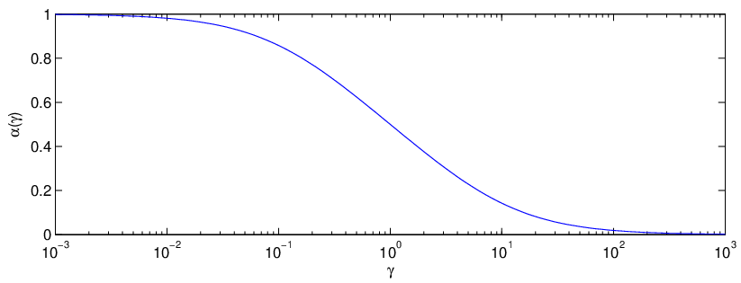
Finally, the preceding discussion can be extended to arbitrary $\gamma>0$ . For every $\gamma>0$ there is a unique $\alpha=\alpha(\gamma)\in(0,1)$ such that

L(y,t)=1_{\{y=1\}}\frac{1}{1+e^{t}}+1_{\{y=-1\}}\frac{1}{\gamma}\frac{1}{1+e^{-\gamma t}}

(14)

is $\alpha$ -CC. The relationship between $\alpha$ and $\gamma$ is shown in Figure 7. Calculation of this curve is discussed in Appendix B. In the appendix we show that $\alpha(\mbox{$\frac{1}{\gamma}$})=1-\alpha(\gamma)$ , which explains the sigmoidal shape of $\alpha$ as a function¹¹ 1 We investigated whether $\alpha(\gamma)=1/(1+e^{c\ln\gamma})$ for some $c>0$ , but evidently it does not. of $\ln\gamma$ .

Now suppose $\alpha^{\prime}\in(0,1)$ is the desired cost asymmetry. By Theorem 3, for $L$ in Eqn. (14), $L_{1-\alpha(\gamma)}$ is CC, and therefore $L_{(1-\alpha(\gamma))\alpha^{\prime}}$ is $\alpha^{\prime}$ -CC. This is a family of losses, indexed by $\gamma>0$ , all of which are $\alpha^{\prime}$ -CC.

5 Discussion

The results of Bartlett et al. (2006) concerning surrogate regret bounds and classification calibration are generalized to label-dependent misclassification costs and arbitrary losses. Some differences that emerge in this more general framework are that $H_{L,\alpha}(\eta)$ is in general not symmetric about $\eta=\frac{1}{2}$ , and $\nu_{L,\alpha}(\epsilon)$ is potentially discontinuous at $\epsilon=\min(\alpha,1-\alpha)$ . The framework of Steinwart (2007) is also applied. Although his notion of calibration is not always equivalent to the one adopted here, that approach based on calibration functions nonetheless leads to the same surrogate regret bounds.

The class of uneven margin losses are examined in some detail. We hope these results provide guidance to future work with such losses, as our theory explains how to ensure $\alpha$ -classification calibration for any margin asymmetry parameter $\gamma>0$ . For example, Adaboost is often applied to heavily unbalanced datasets where misclassification costs are label-dependent, such as in cascades for face detection (Viola and Jones, 2002). It should be possible to generalize Adaboost to have an uneven margin (to accommodate unbalanced data) while being $\alpha$ -classification calibrated for any $\alpha\in(0,1)$ . In particular, the uneven exponential loss from Sec. 4.3 can be optimized by the functional gradient descent approach. In fact, Masnadi-Shirazi and Vasconcelos (2007) developed such an algorithm for the special case $\gamma=\alpha/(1-\alpha)$ , but did not identify the generalization to arbitrary $\gamma$ .

Our theory also sheds light on the support vector machine with uneven margin. Yang et al. (2009) describe an implementation of this algorithm, but they allow for both $\beta$ and $\gamma$ to be free parameters. Our Corollary 2 constrains $\beta=1/\gamma$ for classification calibration, which eliminates a tuning parameter.

In closing, we mention two additional directions for future work. First, an interesting problem related to uneven margin losses is that of surrogate tuning, which in this case is the problem of tuning the parameter $\gamma$ to a particular dataset. Nock and Nielsen (2009) have recently described a data-driven approach to surrogate tuning of classification-calibrated ( $\alpha=\frac{1}{2}$ ) losses. Second, our regret bounds should be applicable to proving the cost-sensitive consistency of algorithms based on surrogate losses.

Acknowledgements

This work was supported in part by NSF Grants CCF-0830490 and CCF-0953135.

Appendix A Lemmas

LSC and USC abbreviate lower semi-continuous and upper semi-continuous.

Lemma 1.

Let $L$ be a loss, $\alpha\in(0,1)$ , and recall $B_{\alpha}=\max(\alpha,1-\alpha)$ .

1.

(a) For any $\eta\in[0,1]$ , $C_{\alpha}^{*}(\eta)=C_{\alpha}(\eta,\eta-\alpha)$ . (b) For any $\eta\in[0,1],t\in\mathbb{R}$ , $C_{\alpha}(\eta,t)-C_{\alpha}^{*}(\eta)=1_{\{\mathop{\mathrm{sign}}(t)\neq\mathop{\mathrm{sign}}(\eta-\alpha)\}}|\eta-\alpha|$ . (c) $R_{\alpha}^{*}=R_{\alpha}(\eta-\alpha)$ . (d) For any $f\in{\cal F}$ ,

R_{\alpha}(f)-R_{\alpha}^{*}=E_{X}[1_{\{\mathop{\mathrm{sign}}(f(X))\neq\mathop{\mathrm{sign}}(\eta(X)-\alpha)\}}|\eta(X)-\alpha|].

2.

(a) $C_{L}^{*}(\eta)$ is concave on $[0,1]$ . (b) $C_{L,\alpha}^{-}(\eta)$ is concave on $[0,\alpha)$ and on $(\alpha,1]$ .

3.

(a) $C_{L}(\eta)$ is continuous on $[0,1]$ . (b) $C_{L,\alpha}^{-}(\eta)$ and $H_{L,\alpha}(\eta)$ are continuous on $[0,1]\backslash\{\alpha\}$ . (c) If $L$ is $\alpha$ -CC, then $C_{L,\alpha}^{-}$ and $H_{L,\alpha}$ are continuous on $[0,1]$ .

4.

$H_{L,\alpha}(\alpha)=\nu_{L,\alpha}(0)=\mu_{L,\alpha}(0)=\psi_{L,\alpha}(0)=0$ .

5.

$\nu_{L,\alpha}$ and $\mu_{L,\alpha}$ are LSC on $[0,B_{\alpha}]$ . $\psi_{L,\alpha}$ is continuous on $[0,B_{\alpha}]$ .

Proof.

1. For $\eta\in[0,1]$ , $C_{\alpha}(\eta,t)=(1-\alpha)\eta 1_{\{t\leq 0\}}+\alpha(1-\eta)1_{\{t>0\}}$ is minimized by any $t$ such that $\mathop{\mathrm{sign}}(t)=\mathop{\mathrm{sign}}((1-\alpha)\eta-\alpha(1-\eta))=\mathop{\mathrm{sign}}(\eta-\alpha)$ . Therefore $C_{\alpha}(\eta,\eta-\alpha)=C_{\alpha}^{*}$ . This gives (a). It also implies

$\displaystyle C_{\alpha}(\eta,t)-C_{\alpha}^{*}(\eta)$
	$\displaystyle=$	$\displaystyle(1-\alpha)\eta 1_{\{t\leq 0\}}+\alpha(1-\eta)1_{\{t>0\}}-[(1-\alpha)\eta 1_{\{\eta\leq\alpha\}}+\alpha(1-\eta)1_{\{\eta>\alpha\}}]$
	$\displaystyle=$	$\displaystyle 1_{\{\mathop{\mathrm{sign}}(t)\neq\mathop{\mathrm{sign}}(\eta-\alpha)\}}\|\eta-\alpha\|,$

which is (b). Part (c) now follows from (a) and $R_{\alpha}^{*}=E_{X}[C_{\alpha}^{*}(\eta(X))]=E_{X}[C_{\alpha}(\eta(X),\eta(X)-\alpha)]=R_{\alpha}(\eta-\alpha)$ , while (d) follows from (b) and

	$\displaystyle R_{\alpha}(f)-R_{\alpha}^{*}$	$\displaystyle=$	$\displaystyle E_{X}[C_{\alpha}(\eta(X),f(X))-C_{\alpha}^{*}(\eta(X))]$
		$\displaystyle=$	$\displaystyle E_{X}[1_{\{\mathop{\mathrm{sign}}(f(X))\neq\mathop{\mathrm{sign}}(\eta(X)-\alpha)\}}\|\eta(X)-\alpha\|].$

2. Since $C_{L}^{*}(\eta)=\inf_{t\in\mathbb{R}}\eta L_{1}(t)+(1-\eta)L_{-1}(t)$ , it is the infimum of affine functions and therefore concave. For $\eta<\alpha$ , $C_{L,\alpha}^{-}(\eta)=\inf_{t\geq 0}C_{L}(\eta,t)$ which is also concave by the same reasoning. A similar argument applies when $\eta>\alpha$ .

3. Since $C_{L}^{*}(\eta)$ is concave on $[0,1]$ , it is continuous on $(0,1)$ by Theorem 10.1 of Rockafellar (1970). By Theorem 10.2 of the same, $C_{L}^{*}$ is LSC at 0 and 1. Let us argue that $C_{L}^{*}$ is USC at 1, the case of 0 being similar. Thus, let $\epsilon>0$ and let $t_{\epsilon}\in\mathbb{R}$ such that $L_{1}(t_{\epsilon})\leq C_{L}^{*}(1)+\frac{\epsilon}{2}$ . If $L_{-1}(t_{\epsilon})=0$ , then for any $\eta\in[0,1)$ , $C_{L}^{*}(\eta)\leq C_{L}(\eta,t_{\epsilon})=\eta L_{1}(t_{\epsilon})\leq L_{1}(t_{\epsilon})\leq C_{L}^{*}(1)+\epsilon$ . Suppose $L_{-1}(t_{\epsilon})>0$ . If $\eta$ is such that $1-\frac{\epsilon}{2L_{-1}(t_{\epsilon})}\leq\eta<1$ , then $C_{L}^{*}(\eta)\leq\eta L_{1}(t_{\epsilon})+(1-\eta)L_{-1}(t_{\epsilon})\leq C_{L}^{*}(1)+\epsilon$ . Thus $C_{L}^{*}$ is USC at 1. This establishes (a).

For (b), continuity of $C_{L,\alpha}^{-}$ on $[0,1]\backslash\{\alpha\}$ follows by a similar argument as (a). Continuity of $H_{L,\alpha}$ then follows immediately.

It remains to show that $C_{L,\alpha}^{-}$ , and hence $H_{L,\alpha}$ , is continuous at $\alpha$ when $L$ is $\alpha$ -CC. First note that $C_{L,\alpha}^{-}$ is LSC at $\alpha$ because $C_{L,\alpha}^{-}(\alpha)=C_{L}^{*}(\alpha)$ , $C_{L,\alpha}^{-}(\eta)\geq C_{L}^{*}(\eta)$ for all $\eta\in[0,1]$ , and from parts (a) and (b).

We now show $C_{L,\alpha}^{-}$ is USC at $\alpha$ when $L$ is $\alpha$ -CC. Let $\epsilon>0$ . Since $C_{L}^{*}$ is continuous at $\alpha$ , there exists $\delta^{\prime}>0$ such that $|C_{L}^{*}(\eta)-C_{L}^{*}(\alpha)|<\frac{\epsilon}{3}$ whenever $|\eta-\alpha|<\delta^{\prime}$ . Let $\delta_{\alpha}=\frac{1}{2}\min(\alpha,1-\alpha),M=\max(L_{1}(0),L_{-1}(0))$ , and set $\delta=\min(\delta^{\prime},\delta_{\alpha},\frac{\epsilon}{3}\cdot\frac{\delta_{\alpha}}{2M})$ . Now suppose $|\eta-\alpha|<\delta$ , $\eta\neq\alpha$ . Then

	$\displaystyle C_{L,\alpha}^{-}(\eta)-C_{L,\alpha}^{-}(\alpha)$	$\displaystyle=$	$\displaystyle C_{L,\alpha}^{-}(\eta)-C_{L}^{}(2\alpha-\eta)+C_{L}^{}(2\alpha-\eta)-C_{L}^{*}(\alpha)$
		$\displaystyle\leq$	$\displaystyle C_{L,\alpha}^{-}(\eta)-C_{L}^{*}(2\alpha-\eta)+\frac{\epsilon}{3},$

since $|(2\alpha-\eta)-\alpha|=|\eta-\alpha|<\delta\leq\delta^{\prime}$ . Since $L$ is $\alpha$ -CC, there exists $t^{*}$ , depending possibly on $\eta$ and $\epsilon$ , such that $t^{*}((2\alpha-\eta)-\alpha)\geq 0$ and $C_{L}(2\alpha-\eta,t^{*})\leq C_{L}^{*}(2\alpha-\eta)+\frac{\epsilon}{3}$ . We may further stipulate $C_{L}(2\alpha-\eta,t^{*})\leq C_{L}(2\alpha-\eta,0)$ which will be needed later. Notice $t^{*}((2\alpha-\eta)-\alpha)\geq 0\iff t^{*}(\eta-\alpha)\leq 0$ , which is also used later. Now $C_{L,\alpha}^{-}(\eta)-C_{L}^{*}(2\alpha-\eta)\leq C_{L,\alpha}^{-}(\eta)-C_{L}(2\alpha-\eta,t^{*})+\frac{\epsilon}{3}$ . Thus far we have shown $C_{L,\alpha}^{-}(\eta)-C_{L,\alpha}^{-}(\alpha)\leq C_{L,\alpha}^{-}(\eta)-C_{L}(2\alpha-\eta,t^{*})+\frac{2\epsilon}{3}$ for $|\eta-\alpha|<\delta,\eta\neq\alpha$ .

Now consider

$\displaystyle C_{L,\alpha}^{-}(\eta)-C_{L}(2\alpha-\eta,t^{})=\inf_{t\in\mathbb{R}:t(\eta-\alpha)\leq 0}C_{L}(\eta,t)-C_{L}(2\alpha-\eta,t^{})$
	$\displaystyle\leq$	$\displaystyle C_{L}(\eta,t^{})-C_{L}(2\alpha-\eta,t^{})$
	$\displaystyle=$	$\displaystyle\eta L_{1}(t^{})+(1-\eta)L_{1}(t^{})-[(2\alpha-\eta)L_{1}(t^{})+(1-(2\alpha-\eta))L_{-1}(t^{})]$
	$\displaystyle=$	$\displaystyle 2[L_{1}(t^{})(\eta-\alpha)+L_{-1}(t^{})(\alpha-\eta)]$
	$\displaystyle\leq$	$\displaystyle 2[L_{1}(t^{})+L_{-1}(t^{})]\|\eta-\alpha\|.$

To bound this quantity, observe

$\displaystyle M$	$\displaystyle=$	$\displaystyle\max(L_{1}(0),L_{-1}(0))$
	$\displaystyle\geq$	$\displaystyle C_{L}(2\alpha-\eta,0)$
	$\displaystyle\geq$	$\displaystyle C_{L}(2\alpha-\eta,t^{*})$
	$\displaystyle=$	$\displaystyle(2\alpha-\eta)L_{1}(t^{})+(1-(2\alpha-\eta))L_{-1}(t^{})$
	$\displaystyle\geq$	$\displaystyle\frac{\alpha}{2}L_{1}(t^{})+\frac{1-\alpha}{2}L_{-1}(t^{})$
	$\displaystyle\geq$	$\displaystyle\delta_{\alpha}(L_{1}(t^{})+L_{-1}(t^{})).$

To see the next to last inequality, recall $|\eta-\alpha|<\delta\leq\delta_{\alpha}=\frac{1}{2}\min(\alpha,1-\alpha)$ . Then $2\alpha-\eta=\alpha+(\alpha-\eta)\geq\frac{\alpha}{2}$ and $1-(2\alpha-\eta)=1-\alpha+(\eta-a)\geq\frac{1-\alpha}{2}$ We now have $C_{L,\alpha}^{-}(\eta)-C_{L}(2\alpha-\eta,t^{*})\leq\frac{2M}{\delta_{\alpha}}|\eta-\alpha|<\frac{\epsilon}{3}$ .

We have shown that for all $\epsilon>0$ , there exist $\delta>0$ such that for all $\eta\in[0,1]$ with $|\eta-\alpha|<\delta$ and $\eta\neq\alpha$ ,

C_{L,\alpha}^{-}(\eta)-C_{L,\alpha}^{-}(\alpha)<\epsilon.

Therefore $C_{L,\alpha}^{-}$ is USC, and hence continuous, at $\alpha$ .

4. $H_{L,\alpha}(\alpha)=0$ because when $\eta=\alpha$ , the infimum defining $C_{L,\alpha}^{-}(\alpha)$ is unrestricted. From this we have $\nu_{L,\alpha}(0)=H_{L,\alpha}(\alpha)=0$ . Since $0\leq\mu_{L,\alpha}(0)\leq\nu_{L,\alpha}(0)$ we deduce $\mu_{L,\alpha}(0)=0$ . Finally, $\psi_{L,\alpha}(0)=0$ because $\psi_{L,\alpha}=\nu_{L,\alpha}^{**}$ , $\nu_{L,\alpha}(0)=0$ , and $\nu_{L,\alpha}$ is nonnegative.

5. From 3, $H_{L,\alpha}$ is continuous except possibly at $\alpha$ . Therefore $\nu_{L,\alpha}$ is continuous except possibly at $0$ and $b_{\alpha}:=\min(\alpha,1-\alpha)$ . $\nu_{L,\alpha}$ is LSC at $0$ because $\nu_{L,\alpha}(0)=0$ and $\nu_{L,\alpha}$ is nonnegative. $\nu_{L,\alpha}$ is LSC at $b_{\alpha}$ because $\nu_{L,\alpha}(b_{\alpha}^{-})=\nu_{L,\alpha}(b_{\alpha})\leq\nu_{L,\alpha}(b_{\alpha}^{+})$ , which follows from the definition of $\nu_{L,\alpha}$ . Now lower semi-continuity of $\mu_{L,\alpha}$ follows from Lemma 2. ∎

The following result generalizes Lemma A.7 of Steinwart (2007).

Lemma 2.

Let $\delta:[0,B]\to[0,\infty)$ be a lower semi-continuous function with $\delta(0)=0$ , and define $\tilde{\delta}(\epsilon)=\inf_{\epsilon^{\prime}\geq\epsilon}\delta(\epsilon^{\prime})$ . Then $\tilde{\delta}$ is lower semi-continuous and $\tilde{\delta}^{**}=\delta^{**}$ .

Proof.

Suppose $\tilde{\delta}$ is not LSC at $\epsilon\in[0,1]$ . Then there exists $\tau>0$ and $\epsilon_{1},\epsilon_{2},\ldots\to\epsilon$ such that for $i$ sufficiently large, $\tilde{\delta}(\epsilon_{i})\leq\tilde{\delta}(\epsilon)-\tau$ . Since $\tilde{\delta}$ is nondecreasing, we may assume $\epsilon_{i}<\epsilon$ for all $i$ . If $\tilde{\delta}(\epsilon_{i})\leq\tilde{\delta}(\epsilon)-\tau$ , then there exists $\epsilon_{i}^{\prime}\in[\epsilon_{i},\epsilon)$ such that $\delta(\epsilon_{i}^{\prime})\leq\tilde{\delta}(\epsilon)-\frac{\tau}{2}\leq\delta(\epsilon)-\frac{\tau}{2}$ . But $\epsilon_{i}^{\prime}\to\epsilon$ , which implies $\delta$ is not LSC at $\epsilon$ , a contradiction.

To show $\tilde{\delta}^{**}=\delta^{**}$ , we need to show $\overline{\mathop{\mbox{\rm co}}\mathop{\mbox{\rm Epi}}\tilde{\delta}}=\overline{\mathop{\mbox{\rm co}}\mathop{\mbox{\rm Epi}}\delta}$ . It suffices to show $\mathop{\mbox{\rm co}}\mathop{\mbox{\rm Epi}}\tilde{\delta}=\mathop{\mbox{\rm co}}\mathop{\mbox{\rm Epi}}\delta$ . Since $\tilde{\delta}\leq\delta$ , clearly $\mathop{\mbox{\rm Epi}}\tilde{\delta}\subset\mathop{\mbox{\rm Epi}}\delta$ and therefore $\mathop{\mbox{\rm co}}\mathop{\mbox{\rm Epi}}\tilde{\delta}\subset\mathop{\mbox{\rm co}}\mathop{\mbox{\rm Epi}}\delta$ . For the reverse inclusion, it suffices to show $(\epsilon,\tilde{\delta}(\epsilon))\in\mathop{\mbox{\rm co}}\mathop{\mbox{\rm Epi}}\delta$ for all $\epsilon\in[0,B]$ . We may assume $\epsilon\in(0,B)$ since $\delta(0)=\tilde{\delta}(0)=0$ and $\delta(B)=\tilde{\delta}(B)$ . Thus let $\epsilon\in(0,B)$ . Since $\delta$ is LSC, it achieves its infimum over a compact set, and hence there exists $\epsilon^{\prime}\in[\epsilon,B]$ such that $\tilde{\delta}(\epsilon)=\delta(\epsilon^{\prime})$ . Since $(0,0),(\epsilon^{\prime},\frac{\epsilon^{\prime}}{\epsilon}\tilde{\delta}(\epsilon))\in\mathop{\mbox{\rm Epi}}(\delta)$ , it follows that

\frac{\epsilon}{\epsilon^{\prime}}(\epsilon^{\prime},\frac{\epsilon^{\prime}}{\epsilon}\tilde{\delta}(\epsilon))+\frac{\epsilon^{\prime}-\epsilon}{\epsilon^{\prime}}(0,0)=(\epsilon,\tilde{\delta}(\epsilon))\in\mathop{\mbox{\rm co}}\mathop{\mbox{\rm Epi}}\delta,

as was to be shown ∎

Appendix B Uneven Sigmoid Loss Details

We present a closed form expression for $t_{-}(\eta)$ , and describe how to calculate $\alpha(\gamma)$ from Sec. 4.4.

$t_{-}(\eta)$ is the value of $t$ that satisfies $t<0$ and

0=\frac{\partial}{\partial t}C_{L}(\eta,t)=\eta\phi^{\prime}(t)-(1-\eta)\phi^{\prime}(-2t).

Using $\phi^{\prime}(t)=-e^{t}/(1+e^{t})^{2}$ and substituting $z=e^{t}$ , $z$ must satisfy $z\in(0,1)$ and

\eta\frac{z}{(1+z)^{2}}=(1-\eta)\frac{z^{-2}}{(1+z^{-2})^{2}},

or equivalently, $z\in(0,1)$ is a solution of the quartic equation

	$\displaystyle 0$	$\displaystyle=$	$\displaystyle\eta z^{4}-(1-\eta)z^{3}+2(2\eta-1)z^{2}-(1-\eta)z+\eta$
		$\displaystyle=$	$\displaystyle z^{2}(\eta z^{2}-(1-\eta)z+2(2\eta-1)-(1-\eta)z^{-1}+\eta z^{-2}).$

Note $z=0$ is not the desired solution, as it corresponds to $t=-\infty$ . Let $w=z+z^{-1}$ , and observe $w^{2}=z^{2}+2+z^{-2}$ . Then $z$ must satisfy

$\displaystyle 0$	$\displaystyle=$	$\displaystyle\eta(z^{2}+z^{-2})-(1-\eta)(z+z^{-1})+2(2\eta-1)$
	$\displaystyle=$	$\displaystyle\eta(w^{2}-2)-(1-\eta)w+2(2\eta-1)$
	$\displaystyle=$	$\displaystyle\eta w^{2}-(1-\eta)w+2\eta-1.$

Therefore

w=\frac{1-\eta+\sqrt{(1-\eta)^{2}-8\eta(\eta-1)}}{2\eta}.

We take the positive sign because only it gives a positive $z$ . Now $z$ can be recovered from $w$ . Since $z^{2}-wz+1=0$ we get

z=\frac{w-\sqrt{w^{2}-4}}{2}.

We take the negative sign as we are seeking the smaller of the two critical points. It can be shown (with algebra) that $w^{2}>4\iff\eta<\frac{1}{2}$ . Finally, we have $t_{-}(\eta)=\ln z$ .

We now turn to characterization of $\alpha(\gamma)$ . Assume $\gamma>1$ . $\alpha(\gamma)$ is the value of $\eta$ such that

\frac{1-\eta}{\gamma}=C_{L}(\eta,\infty)=C_{L}(\eta,t)=\frac{\eta}{1+e^{t}}+\frac{1-\eta}{\gamma}\frac{1}{1+e^{-\gamma t}}

is satisfied by a unique $t$ with $-\infty<t<0$ . Since $C_{L}(\eta,-\infty)=C_{L}(\eta,\infty)\iff\eta=\frac{1}{1+\gamma}$ , we must have $\eta>\frac{1}{1+\gamma}$ . After substituting $z=e^{t}$ and simplifying, we seek $\eta>\frac{1}{1+\gamma}$ such that

\eta\gamma z^{\gamma}-(1-\eta)z+(\eta\gamma-1+\eta)=0

is satisfied for a unique $z\in(0,1)$ . That is, we need the curves $p_{\eta}(z):=\eta\gamma z^{\gamma}$ and $q_{\eta}(z):=(1-\eta)z-(\eta\gamma-1+\eta)$ to intersect exactly once on $(0,1)$ . Since $p_{\eta}$ is a strictly increasing convex function and $q_{\eta}$ is a line with positive slope, this can happen in one of three ways: (a) $p_{\eta}(0)>q_{\eta}(0)$ and $p_{\eta}(1)<q_{\eta}(1)$ , (b) $p_{\eta}(0)<q_{\eta}(0)$ and $p_{\eta}(1)>q_{\eta}(1)$ , or (c) $q_{\eta}$ is tangent to $p_{\eta}$ at some $z\in(0,1)$ . (a) requires $\eta>1/(1+\gamma)$ and $\eta<1/(1+\gamma)$ , which is impossible. Similarly, (b) is impossible. Thus, we must have $p_{\eta}^{\prime}(z)=q_{\eta}^{\prime}(z)$ for some $z\in(0,1)$ .

Summarizing up to this point, we seek $\eta>\frac{1}{1+\gamma}$ and $z\in(0,1)$ such that

\eta\gamma z^{\gamma}=(1-\eta)z-(\eta\gamma-1+\eta)

(15)

and

\eta\gamma^{2}z^{\gamma-1}=1-\eta.

(16)

Dividing (15) by (16) and solving for $z$ gives

z=\frac{\eta\gamma-1+\eta}{1-\eta}\frac{\gamma}{\gamma-1}.

(17)

Substituting (17) into (16) yields

\eta\left[\gamma^{2}\left(\frac{\eta\gamma-1+\eta}{1-\eta}\frac{\gamma}{\gamma-1}\right)^{\gamma-1}+1\right]=1.

(18)

When $\gamma=2$ , this simplifies to a quadratic equation, leading to $\alpha(2)=(3+4\sqrt{2})/23$ . More generally, notice that for $\eta>\frac{1}{1+\gamma}$ , the left-hand side of (18) is strictly increasing, and thus $\eta=\alpha(\gamma)$ can be found with a bisection search. The case $\gamma=1$ was treated by Bartlett et al. (2006), yielding $\alpha(1)=\frac{1}{2}$ . When $\gamma<1$ we may appeal to symmetry. Let us write $C_{L}^{\gamma}(\eta,t)$ to indicate the dependence of $C_{L}$ on $\gamma$ . It is easily shown that $C_{L}^{1/\gamma}(\eta,\gamma t)=\gamma C_{L}^{\gamma}(1-\eta,-t)$ , from which it follows that $\alpha(\frac{1}{\gamma})=1-\alpha(\gamma)$ .

References

Bartlett et al. [2006] P. Bartlett, M. Jordan, and J. McAuliffe. Convexity, classification, and risk bounds. J. Amer. Statist. Assoc., 101(473):138–156, 2006.
Li and Shawe-Taylor [2003] Y. Li and J. Shawe-Taylor. The SVM with uneven margins and chinese document categorisation. In In Proceedings of The 17th Pacific Asia Conference on Language, Information and Computation, pages 216–227, 2003.
Li et al. [2002] Y. Li, H. Zaragoza, R. Herbrich, J. Shawe-Taylor, and J. Kandola. The perceptron algorithm with uneven margins. In Proceedings of the Nineteenth International Conference on Machine Learning, pages 379–386, 2002.
Masnadi-Shirazi and Vasconcelos [2007] H. Masnadi-Shirazi and N. Vasconcelos. Asymmetric boosting. In Proceedings of International Conference on Machine Learning, pages 609–619, 2007.
Nock and Nielsen [2009] R. Nock and F. Nielsen. On the efficient minimization of classification calibrated surrogates. In D. Koller, editor, Advances in Neural Information Processing Systems 21, pages 1201–1208, 2009.
Reid and Williamson [2009a] M. D. Reid and R. C. Williamson. Surrogate regret bounds for proper losses. In Proceedings of the 26th Annual International Conference on Machine Learning, pages 897–904, 2009a.
Reid and Williamson [2009b] M. D. Reid and R. C. Williamson. Composite binary losses. Technical report, arXiv:0912.3301v1, December 2009b.
Rockafellar [1970] R. T. Rockafellar. Convex Analysis. Princeton University Press, Princeton, NJ., 1970.
Steinwart [2005] I. Steinwart. Consistency of support vector machines and other regularized kernel classifiers. IEEE Trans. Inform. Theory, 51(1):128–142, 2005.
Steinwart [2007] I. Steinwart. How to compare different loss functions and their risks. Constructive Approximation, 26(2):225–287, 2007.
Viola and Jones [2002] P. Viola and M. Jones. Fast and robust classification using asymmetric adaboost and a detector cascade. In T. G. Dietterich, S. Becker, and Z. Ghahramani, editors, Advances in Neural Information Processing Systems 14, Cambridge, MA, 2002. MIT Press.
Yang et al. [2009] C. Yang, J. Yang, and J. Wang. Margin calibration in SVM class-imbalanced learning. Neurocomputing, 73(1-3):397–411, 2009.
Zhang [2004] T. Zhang. Statistical behavior and consistency of classification methods based on convex risk minimization. The Annals of Statistics, 32(1):56–85, 2004.

$\displaystyle C_{L,\alpha}^{-}(\eta)-C_{L}(2\alpha-\eta,t^{})=\inf_{t\in\mathbb{R}:t(\eta-\alpha)\leq 0}C_{L}(\eta,t)-C_{L}(2\alpha-\eta,t^{})$
	$\displaystyle\leq$	$\displaystyle C_{L}(\eta,t^{})-C_{L}(2\alpha-\eta,t^{})$
	$\displaystyle=$	$\displaystyle\eta L_{1}(t^{})+(1-\eta)L_{1}(t^{})-[(2\alpha-\eta)L_{1}(t^{})+(1-(2\alpha-\eta))L_{-1}(t^{})]$
	$\displaystyle=$	$\displaystyle 2[L_{1}(t^{})(\eta-\alpha)+L_{-1}(t^{})(\alpha-\eta)]$
	$\displaystyle\leq$	$\displaystyle 2[L_{1}(t^{})+L_{-1}(t^{})]\|\eta-\alpha\|.$

Calibrated Surrogate Losses for Classification with Label-Dependent Costs

Abstract

1 Introduction

2 Surrogate Losses and Regret Bounds

2.1 α\alpha-classification calibration and surrogate regret bounds

Definition 1.

Theorem 1.

Proof.

Corollary 1.

Proof.

2.2 Cost-insensitive classification

Definition 2.

Theorem 2.

Proof.

Theorem 3.

Proof.

2.3 Convex partial losses

Theorem 4.

Proof.

Theorem 5.

Proof.

3 Calibration Functions

Definition 3.

Theorem 6.

Proof.

Theorem 7.

Proof.

Theorem 8.

Proof.

Theorem 9.

Proof.

4 Uneven Margin Losses

Definition 4.

Corollary 2.

Proof.

4.1 Uneven hinge loss

4.2 Uneven squared error loss

4.3 Uneven exponential loss

4.4 Uneven sigmoid loss

5 Discussion

Acknowledgements

Appendix A Lemmas

Lemma 1.

Proof.

Lemma 2.

Proof.

Appendix B Uneven Sigmoid Loss Details

References

2.1 $\alpha$ -classification calibration and surrogate regret bounds