Joint Channel Probing and Proportional Fair Scheduling in Wireless Networks

Hui Zhou, Pingyi Fan, Dongning Guo Note: H. Zhou and P. Fan are with the Department of Electronic Engineering, Tsinghua University, Beijing, 100084, China (e-mail: h-zhou03@mails.thu.edu.cn; fpy@tsinghua.edu.cn)
D. Guo is with the Department of Electrical Engineering and Computer Science, Northwestern University, Evanston, IL 60208, U.S.A. (e-mail: dguo@northwestern.edu) Affiliation:

Abstract

The design of a scheduling scheme is crucial for the efficiency and user-fairness of wireless networks. Assuming that the quality of all user channels is available to a central controller, a simple scheme which maximizes the utility function defined as the sum logarithm throughput of all users has been shown to guarantee proportional fairness. However, to acquire the channel quality information may consume substantial amount of resources. In this work, it is assumed that probing the quality of each user’s channel takes a fraction of the coherence time, so that the amount of time for data transmission is reduced. The multiuser diversity gain does not always increase as the number of users increases. In case the statistics of the channel quality is available to the controller, the problem of sequential channel probing for user scheduling is formulated as an optimal stopping time problem. A joint channel probing and proportional fair scheduling scheme is developed. This scheme is extended to the case where the channel statistics are not available to the controller, in which case a joint learning, probing and scheduling scheme is designed by studying a generalized bandit problem. Numerical results demonstrate that the proposed scheduling schemes can provide significant gain over existing schemes.

I Introduction

Efficient and fair scheduling is important for wireless systems with limited resources and heterogeneous user conditions. A large class of resource allocation schemes with fairness considerations are obtained by maximizing some utility functions of the throughput [1]. In particular, proportional fairness is achieved when the utility is the sum of the logarithm of the users’ throughput. In existing third generation wireless systems, like EV-DO and HSDPA, proportional fair (PF) scheduling scheme is employed at the base station to schedule downlink traffic to mobile users. The PF scheme strikes a good balance between throughput efficiency and fairness by exploiting the multiuser diversity [2] and the game-theoretic equilibrium [3]. Analysis and applications on PF scheduling have been extensively explored from various aspects due to its favorable performance and low implementation complexity. For example, there have been studies of the convergence and optimality [4], stability [5], throughput [6] and capacity region [7] of PF scheduling.

Most previous work on PF scheduling assume that the instantaneous channel quality information (CQI) of all users is known to the scheduler at no cost. In practice, however, acquiring the CQI often consumes a significant amount of resources in terms of time, bandwidth and power. It is important to understand the impact of the cost when the number of users is large, because the cost may scale linearly with the user population. The goal of this work is to answer the following two questions: 1) to what extent will the CQI acquisition affect the scheduling? and 2) how to probe and schedule the users to achieve the best performance with proportional fairness?

There have been related works on the impact of the channel uncertainty on the communication systems. The loss of throughput caused by poor estimates of channel quality is quantified in [8]. Joint channel probing and user scheduling has also been addressed recently. Several schemes with the objective of maximizing the system throughput have been designed in [9, 10, 11, 12]. And the authors of [13, 14, 15] propose schemes for stabilizing the queues and characterize the network throughput region. In contrast to the preceding works, the goal of this paper is to design a proportional fair scheduling scheme which takes into account the cost of channel probing. Our previous work [16] has shown the scheme and its performance roughly. In this paper, we not only present the derivation of the scheme with rigorous arguments, but also show its asymptotic behavior and the optimality with theoretical rigor. In addition, the scheme is extended to a more generalized scenario. The organization and main contributions of this work are as follows:

•

Section II describes the network model.
•

In Section III, we assume the prior distribution of CQI is known to the scheduler, and formulate the problem of sequentially probing user channels to make scheduling decision as a stopping time problem. A simple scheme based on maximizing the sum logarithm throughput of all users is shown to guarantee proportional fairness and convergence. The scheduling gain of the scheme is determined analytically. Further reduction of computational complexity is also discussed.
•

In Section IV, the statistics of the CQI is assumed not to be available to the scheduler. The problem is formulated as a generalized bandit problem, and a joint learning, probing and scheduling scheme is proposed.
•

In Section V, significant advantages of the proposed schemes are demonstrated using numerical experiments. In typical scenarios where the statistics of the CQI are not available, the joint learning, probing and scheduling scheme achieves almost the same performance as that in the case where the statistics are known.

II The Network Model

Consider a wireless system with one controller and $K$ users with time-varying channel quality, such as in the downlink of a cellular system. Let time be divided into unit-length slots and only one user can be served in each slot. As in most related work (e.g., [4] and [6]), the transmit power is assumed to be fixed so that dynamic power allocation is not considered. Thus the achievable rate is only determined by the instantaneous channel quality. Moreover, we assume saturated traffic for all users.

Assume slow fading, where the duration of a slot is much shorter than the channel coherence time, so that the channel quality remains constant during each slot. We make the following homogeneous rate assumption that the rate of each user normalized by its mean value follows the same distribution:

(A1) Let $X_{1},\dots,X_{K}$ be independent identically distributed (i.i.d.) non-negative random variables with unit mean value. Let $r_{1},\dots,r_{K}\geq 0$ be constants. Let $R_{k}=r_{k}X_{k}$ for $k=1,\dots,K$ . The achievable rates $\{R_{k}(n)|k=1,\dots,K;n=1,2,\dots\}$ are independent. For every user $k$ , the rates over the time slots, $R_{k}(1),R_{k}(2),\dots$ , are i.i.d. following the same distribution as that of $R_{k}$ . Clearly, $\mathbb{E}R_{k}(n)=r_{k}$ .

The instantaneous achievable rates of all users are not known a priori. During each slot $n$ , to obtain the achievable rate $R_{k}(n)$ requires the scheduler to probe the channel of user $k$ using a fraction $\beta$ of the slot. Let $I_{k}(n)$ be an indicator of the event that user $k$ is scheduled for transmission in slot $n$ . Let $J(n)$ denote the number of probed users in slot $n$ . The amount of data transmitted to or by user $k$ during slot $n$ is $B_{k}(n)=(1-J(n)\beta)R_{k}(n)I_{k}(n),$ which is nonzero for only one user during each slot. The throughput of user $k$ averaged over $n$ slots is thus

T_{k}(n)=\frac{1}{n}\sum^{n}_{j=1}B_{k}(j).

(1)

III Joint Probing and Scheduling with Known Channel Statistics

In this section, we consider the case where the statistics of $\bm{R}=[R_{1},\dots,R_{K}]$ is known to the scheduler and design a proportional fair scheme.

III-A The Algorithm

Consider first a scheme which maximizes the utility defined as the sum logarithm throughput:

\displaystyle u(\bm{T}(n))=\sum^{K}_{k=1}\ln T_{k}(n)\ .

(2)

Note that by (1),

T_{k}(n)=\frac{n-1}{n}T_{k}(n-1)+\frac{1}{n}B_{k}(n).

(3)

So that the increase of the utility function after the $n$ -th slot is

	$\displaystyle u(\bm{T}(n))-u(\bm{T}(n-1))$
$\displaystyle=$	$\displaystyle\sum_{k=1}^{K}(\ln T_{k}(n)-\ln T_{k}(n-1))$
$\displaystyle=$	$\displaystyle\sum_{k=1}^{K}\ln\left(\frac{n-1}{n}+\frac{1}{n}\frac{B_{k}(n)}{T_{k}(n-1)}\right)$
$\displaystyle=$	$\displaystyle\sum^{K}_{k=1}\ln\left(\frac{n-1}{n}+\frac{1-\beta J(n)}{n}s_{k}(n)I_{k}(n)\right),$	(4)

where the throughput-normalized rate is

s_{k}(n)=\frac{{R_{k}(n)}}{T_{k}(n-1)}.

(5)

Since the indicator $I_{k}(n)$ is zero for all but one user $k$ in each slot, one can see that to greedily maximize the utility increment at time slot $n$ , we should schedule the user with the maximum $s_{k}(n)$ , which is the classical PF scheduling algorithm.

However, due to the assumption that the instantaneous rates $R_{k}(n)$ are unknown a priori, we can only probe the users rates and obtain $s_{k}(n)$ one by one in each slot. We formulate the following optimal stopping time problem [18]. Note that the scheduling decision made in one slot has no impact on future realization of the rates, it suffices to consider one arbitrary slot and omit the time index $n$ . For the scheduler, the joint probing and scheduling problem at the beginning of the time slot is defined by two objects:

(i) The independent throughput-normalized rates $s_{1},\dots,s_{K}$ .

(ii) A sequence of positive-valued reward functions $y_{1},\dots,y_{K}$ , where if $j$ channels have been probed to reveal their throughput-normalized instantaneous rates $t_{1},\dots,t_{j}$ , the reward of terminating the probing phase and schedule the best user found so far is

y_{j}(t_{1},\dots,t_{j})=(1-j\beta)\max(t_{1},\dots,t_{j}).

(6)

The theory of optimal stopping is concerned with determining the stopping time $J$ to maximize the expected reward $\mathbb{E}[y_{J}]$ . The maximum number of probings in every slot is $J_{max}=\min(K,\left\lfloor 1/\beta\right\rfloor)$ . Compared with the classical optimal stopping problem, the formulation above is more general in the sense that the probing order of $s_{k}$ is not deterministic. Hence the joint probing and scheduling scheme basically includes two tasks in each slot: to determine the order in which users are probed, and to select one user as the destination at a proper (stopping) time. Recalling the objective of maximizing the expected $y_{j}$ , the user with the largest $\mathbb{E}[s_{k}(n)]$ should be probed first, and then the second largest and so on. From Assumption (A1), we know $\bar{s}_{k}(n)\triangleq\mathbb{E}[s_{k}(n)]=r_{k}/T_{k}(n-1)$ . Hence the probing order is $\pi(n)=(k_{1},\cdots,k_{K})$ such that $\bar{s}_{k_{1}}(n)\geq\dots\geq\bar{s}_{k_{K}}(n)$ . Now that the probing order has been determined, the decision on when to stop can be addressed by investigating the structural property of the problem.

Theorem 1

Under the homogeneous rate assumption (A1), the joint probing and scheduling problem is a monotone stopping problem [18, Chapter 5], which means that, if $\mathcal{E}_{j}$ denotes the event

\left\{y_{j}(s_{k_{1}},\cdots,s_{k_{j}})\geq\mathbb{E}[y_{j+1}(s_{k_{1}},\cdots,s_{k_{j+1}})|s_{k_{1}},\cdots,s_{k_{j}}]\right\},

(7)

then $\mathcal{E}_{j}\subseteq\mathcal{E}_{j+1}$ for $0\leq j\leq J_{max}-1$ .

Proof: See appendix A.

Now the problem has been proved to be monotone, then from the [18, Theorem 1, Chapter 5], the one-state look-ahead rule is optimal. The one-stage look-ahead rule is the one that stops if the reward for stopping at current stage is at least as large as the expected reward of continuing one stage and then stop. Mathematically, the rule is described by the stopping time. Let $w_{j}$ denote the largest value of the observed throughput-normalized rate after probing $j$ users and $a\vee b\triangleq\max(a,b)$ , the optimal stopping time is

J^{*}=\min\left\{j\geq 0:(1-j\beta)w_{j}\geq(1-(j+1)\beta)\mathbb{E}\left[w_{j}\vee\frac{R_{k_{j+1}}}{T_{k_{j+1}}(n-1)}\bigg|w_{j}\right]\right\},

(8)

which solves the stopping problem almost surely in each slot. Precisely, the optimal PF joint probing and scheduling (JPS-PF) scheme is described as Algorithm 1.

Algorithm 1 JPS-PF

Initialization:

T_{k}(0)\leftarrow 1

for

k=1,\cdots,K

;

1 for $n=1,2,\cdots$ do

\bar{s}_{k}(n)\leftarrow r_{k}/T_{k}(n-1)

. Sort the throughput-normalized mean rate

\bar{s}_{k}(n)(k=1,\cdots,K)

in the descending order:

\bar{s}_{k_{1}}(n)\geq\dots\geq\bar{s}_{k_{K}}(n)

;

j\leftarrow 0

w\leftarrow 0

;

4 do

j\leftarrow j+1

;

6 Probe user

k_{j}

and get the rate

R_{k_{j}}(n)

;

w\leftarrow w\vee R_{k_{j}}(n)/T_{k_{j}}(n-1)

;

8 while $(1-j\beta)w<(1-(j+1)\beta)\mathbb{E}\left[w\vee\frac{R_{k_{j+1}}}{T_{k_{j+1}}(n-1)}\right]$ ;

9 Transmit to user

k_{j}

. Update

\bm{T}(n)

;

10 end for

III-B On the Optimality of Algorithm 1

To present the optimality of Algorithm 1, we need to show the convergence property.

Theorem 2

Assume (A1). Then for any initial condition, the throughput sequence $\bm{T}(n)$ generated under Algorithm 1 converges almost surely to the limit point $\bm{T}^{*}$ of the ordinary differential equation $\dot{\bm{T}}(t)=\bm{h}(\bm{T}(t))$ , where $\bm{h}(\bm{T})=-\bm{T}+\mathbb{E}[\bm{B}(n)|\bm{T}(n-1)=\bm{T}]$ . Moreover, all users’ steady-state throughput are proportional to their mean rate with an identical ratio $\kappa$ ,

\frac{T_{1}^{*}}{r_{1}}=\frac{T_{2}^{*}}{r_{2}}=\cdots=\frac{T_{K}^{*}}{r_{K}}=\kappa.

(9)

Proof:

Let $\bm{M}(n)=\bm{B}(n)-\mathbb{E}[\bm{B}(n)|\bm{T}(n-1)]$ . By (3), the update of users’ throughput can be organized in the form of stochastic approximation iteration [19, Eqn. 2.1.1]:

\displaystyle\bm{T}(n)=\bm{T}(n-1)+a(n)[\bm{h}(\bm{T}(n-1))+\bm{M}(n)],

where $a(n)=1/n$ . The equation above is a standard stochastic approximation expression. It is easy to verify that $\bm{h}(\cdot)$ is Lipshitz, the stepsize satisfies $\sum_{n}a(n)=\infty,\sum_{n}a(n)^{2}<\infty$ and $\bm{T}(n)$ is bounded. Furthermore, it is easy to verify that $\mathbb{E}[\bm{M}(n)|\bm{M}(1),\cdots,\bm{M}(n-1)]=0$ , so $\bm{M}(n)$ is a martingale difference sequence. Now the throughput update under the proposed scheme satisfies the assumptions (A1)-(A4) in [19, Section 2.1], then applying Theorem 2 in [19, Section 2.1] directly, the convergence conclusion holds.

Now the convergence of the throughput sequence has been obtained. The remainder of the proof is by contradiction. Suppose (9) does not hold at steady state and that ${T_{1}^{*}}/{r_{1}}<{T_{2}^{*}}/{r_{2}}$ without loss of generality. Consider the throughput path starting at slot $n_{0}$ which is at steady state. At this time, $\bar{s}_{l}=r_{l}/T_{l}^{*}(l=1,2)$ and $\bar{s}_{1}>\bar{s}_{2}$ . Thus user $1$ is probed first in each slot. From assumption (A1) we know that $s_{1}$ and $s_{2}$ are of the same type of distribution, but $s_{1}$ has a larger mean value. Thus user $1$ is selected for transmission more often than user $2$ , which would further imply ${T_{1}(n_{0}+n_{1})}/{r_{1}}>{T_{2}(n_{0}+n_{1})}/{r_{2}}$ after a sufficiently large number ( $n_{1}$ ) of slots, which contradicts the steady state assumption with $T_{1}^{*}/r_{1}<T_{2}^{*}/r_{2}$ . ∎

Note that the constant proportionality factor $\kappa$ is a bridge connecting the steady-state throughput and the mean-rate. After obtaining $\kappa$ , it is straightforward to evaluate the throughput and utility. On the other hand, due to the fact that $\kappa$ is a constant, we have the following corollary from the proof of Theorem 2.

Corollary 1

Under Algorithm 1, the probability that each user is selected as the destination is identical as $1/K$ .

Algorithm 1 is asymptotically optimal in the following sense:

Theorem 3

Assume (A1). Then $\bm{T}^{*}$ maximizes the PF utility $u(\cdot)$ over the rate region generated by all joint probing and scheduling schemes.

Proof:

Let $\mathcal{S}$ denote the set composed of all the feasible schemes $\Gamma$ under the assumption that only one user can be selected in one slot. The developed scheme in this paper is denoted as $\Gamma^{*}$ . We have shown in the derivation of Algorithm 1 that $\Gamma^{*}$ is optimal for solving the monotone stopping problem in each slot, that is, it maximizes $B_{k}(n)/T_{k}(n-1)$ in slot $n$ almost surely. Due to the constraint that only one user can be scheduled in one slot, we can see that the developed scheme $\Gamma^{*}$ satisfies

\Gamma^{*}\in\arg\max_{\Gamma\in\mathcal{S}}\sum_{k=1}^{K}\frac{B_{k}^{(\Gamma)}(n)}{T_{k}(n-1)},

(10)

where $B_{k}^{(\Gamma)}(n)$ is the number of bits transmitted to user $k$ in slot $n$ under the scheme $\Gamma$ . Recalling the definition of the utility function in (2), it can be found that

\sum_{k=1}^{K}\frac{B_{k}^{(\Gamma)}(n)}{T_{k}(n-1)}=\nabla u(\bm{T}(n-1))\cdot\bm{B}^{(\Gamma)}(n),

(11)

which means that the scheme chooses a decision maximizing the scalar product of $\bm{B}^{(\Gamma)}(n)$ and the gradient $\nabla u(\bm{T}(n-1))$ .

The gradient scheduling algorithm developed by Stolyar [17] is that, at time $n$ the controller chooses a decision $\Gamma(n)\in\arg\max\limits_{\Gamma}\nabla u(\bm{T}(n-1))\cdot\bm{B}^{(\Gamma)}(n)$ . Let $\tilde{\bm{T}}$ denote the solution to the problem

	$\displaystyle\max$	$\displaystyle\text{~~~~}u(\bm{T})$
	$\displaystyle s.t.$	$\displaystyle\text{~~~~}\bm{T}\in\mathcal{V},$

where $\mathcal{V}$ is the system rate region, i.e., the set of all feasible long-term service rate vectors. Then the [17, Theorem 2] shows that the expected average service rates under the gradient scheduling algorithm converges in probability to $\tilde{\bm{T}}$ .

By (10) and (11), one can see that the joint probing and scheduling algorithm in this paper belongs to the gradient scheduling algorithm. From the convergence of Algorithm 1, we know $\bm{T}^{*}=\tilde{\bm{T}}$ . Then the achieved throughput $\bm{T}^{*}$ maximizes the PF utility function asymptotically. ∎

III-C A Static Threshold Criteria

Note that in Algorithm 1, after each probe, the scheduler needs to evaluate the expectation in (8) which depends on the channel realizations. Further reduction in the computational complexity is possible by simply comparing the highest normalized rate against a sequence of deterministic thresholds, in lieu of computing (8). Consider the steady-state case where users’ throughput is exactly $\bm{T}^{*}$ . Note that by Theorem 2,

\displaystyle\frac{R_{k_{j+1}}}{T_{k_{j+1}}(n-1)}=\frac{R_{k_{j+1}}}{T_{k_{j+1}}^{*}},

which is identically distributed as $X_{1}/\kappa$ . For $0\leq j\leq J_{max}-1$ , the inequality of $w_{j}$ in (8) reduces to

(1-j\beta)w_{j}\geq(1-(j+1)\beta)\mathbb{E}[\max(w_{j},\kappa^{-1}X_{1})|w_{j}].

(12)

It turns out that (12) can be reduced to comparing $\kappa w_{j}$ with a static threshold $v_{j}$ , which can be determined as follows. Let $F_{X}(\cdot)$ denote the cumulative distribution function (CDF) of $X_{k}$ . Then

\displaystyle\mathbb{E}\left[\max\left(w_{j},\frac{X_{1}}{\kappa}\right)\bigg|w_{j}\right]=w_{j}+\int_{\kappa w_{j}}^{\infty}\left(\frac{x}{\kappa}-w_{j}\right)dF_{X}(x).

(13)

So that (12) can be rewritten as

(1-j\beta)w_{j}\geq(1-(j+1)\beta)\left[w_{j}+\int_{\kappa w_{j}}^{\infty}\left(\frac{x}{\kappa}-w_{j}\right)dF_{X}(x)\right],

(14)

or, equivalently,

\kappa w_{j}\geq g_{j}(\kappa w_{j}),

(15)

where

g_{j}(v)=\left[{\beta}^{-1}-(j+1)\right]\int_{v}^{\infty}(x-v)dF_{X}(x).

(16)

It is not hard to check that: (i) $g_{j}(v)>0$ for $v\geq 0$ ; (ii) $g_{j}(v)$ is a strictly decreasing function of $v$ ; (iii) $\lim_{v\rightarrow\infty}g_{j}(v)=0$ . Then inequality (15) is equivalent to $\kappa w_{j}\geq v_{j}$ , where $v_{j}$ is the cross point of function $f(v)=v$ and $g_{j}(v)$ . Also, we have $g_{j}(v)>g_{j+1}(v)$ . Then it is easy to verify that $v_{j+1}<v_{j}$ . The solution to (15) is illustrated in Fig. 2.

By observing the structure of (16), it is worth pointing out that the cross point $v_{j}$ is only determined by $j$ , $\beta$ and the CDF $F_{X}(\cdot)$ , i.e., the unit mean valued random variable $X_{j}$ . And the value of $v_{j}$ is independent of the number of users $K$ , the mean rates of all users $r_{k}$ as well as the achieved throughput to mean-rate ratio $\kappa$ . Hence if the transmitter knows the distribution $F_{X}(\cdot)$ , it can compute $v_{j}$ in advance.

Now inequality (12) can be expressed as $w_{j}\geq\frac{1}{\kappa}v_{j}$ for $0\leq j\leq J_{max}-1$ , which is also equivalent to the inequality in (8) in the steady-state case. Thus the decision on whether to keep probing or to start transmitting is decided by a static threshold criteria. For completeness, let $v_{J_{max}}=0$ in order to make sure the probing can always be terminated in each slot. We get the following static threshold based probing criteria, which can replace the line 9 in Algorithm 1.

Criteria 1: After probing $j$ users, if the current value of the largest normalized rate $w_{j}\geq\frac{1}{\kappa}v_{j}$ , then the transmitter transmits to the user with the largest normalized rate; otherwise it probes the $(j+1)$ st user.

In practice, the scheduler can calculate $v_{j}$ in advance but $\kappa$ is unavailable at the beginning. One way to estimate $\kappa$ is to start the joint probing and scheduling using the dynamic criteria in line 9 of Algorithm 1. After a period of time, the throughput approaches to its steady-state value. Then the throughput to mean-rate ratio $\kappa$ is obtained and the static threshold criteria can be used thereafter. Alternatively, $\kappa$ can be determined theoretically as discussed in the next subsection.

III-D The Scheduling Gain

In this section we analyze the performance of the proposed scheme theoretically. We define the scheduling gain as the ratio of the achieved throughput to that using round robin scheduling without probing, which reflects how much multiuser diversity benefits can be exploited. The scheduling gain of the proposed joint probing and scheduling scheme is $\frac{T_{k}^{*}}{K^{-1}r_{k}}=\kappa K.$ For a random variable $X$ , let us denote the truncation of $X$ over $[a,b]$ as $[X]_{a}^{b}$ . Note that $\mathbb{E}[X|a\leq X\leq b]=\mathbb{E}{[X]_{a}^{b}}$ .

Theorem 4

Under the homogeneous rate assumption (A1), the scheduling gain of Algorithm 1 is

\displaystyle\kappa K

\displaystyle=

\displaystyle\sum_{j=1}^{J_{max}}\left[(F_{X}(v_{j-1}))^{j-1}-(F_{X}(v_{j}))^{j}\right](1-j\beta)\mathbb{E}\left\{\left[\max\left([X_{1}]_{0}^{v_{j-1}},\cdots,[X_{j-1}]_{0}^{v_{j-1}},X_{j}\right)\right]_{v_{j}}^{\infty}\right\},

where $v_{j}$ is the solution of $v=g_{j}(v)$ .

Recall that $J^{*}$ is the optimal stopping time, that is, the number of users probed before a user is scheduled. We prove Theorem 4 using the following supporting lemma.

Lemma 1

Using Algorithm 1, the steady-state probability of the event that $j$ users are probed until transmission is given by

p_{j}={(F_{X}(v_{j-1}))^{j-1}-(F_{X}(v_{j}))^{j}}\text{, }{1\leq j\leqslant J_{max}}.

(17)

Proof:

At steady state, all users’ throughput-normalized mean rates ${r_{k}}/{T_{k}^{*}}$ are essentially identical. Let $q_{j}=\text{Pr}\{J^{*}\geq j\}$ , i.e., the probability that at least $j$ users are probed before transmission. Then $q_{1}=1$ . And from Criteria 1, we have for $j\geq 2$ ,

	$\displaystyle q_{j}$	$\displaystyle=\text{Pr}\{\max(X_{1},\cdots,X_{j-1})<v_{j-1}\}{}$
		$\displaystyle=\text{Pr}\{X_{1}<v_{j-1}\}\cdots\text{Pr}\{X_{j-1}<v_{j-1}\}{}$
		$\displaystyle=(F_{X}(v_{j-1}))^{j-1}.$

Like $v_{j}$ , $q_{j}$ is also completely determined by the rate distribution. Clearly, $p_{j}=q_{j}-q_{j+1}$ for $j\leq J_{max}-1$ and $p_{J_{max}}=q_{J_{max}}$ . ∎

Proof of Theorem 4: Consider a specific user $k$ . In the steady state, $\dot{\bm{T}}(t)=0$ . Then from Theorem 2, user $k$ ’s throughput is given by $T_{k}^{*}=\mathbb{E}[B_{k}(n)|\bm{T}^{*}]$ . Throughout, let $K^{*}$ denote index of the user that is selected as destination. Then event $\{K^{*}=k\}$ , i.e., user $k$ is selected as destination, can be decomposed into $J_{max}$ exclusive sub events: $\{K^{*}=k\}=\bigcup\limits_{j=1,\cdots,J_{max}}\{K^{*}=k,J^{*}=j\}$ . Then we have

	$\displaystyle T_{k}^{*}=$	$\displaystyle\mathbb{E}[B_{k}(n)\|\bm{T}^{}]\stackrel{{\scriptstyle}}{{=}}\mathbb{E}[(1-J^{}\beta)R_{k}I_{k}]{}$
	$\displaystyle{}\stackrel{{\scriptstyle}}{{=}}$	$\displaystyle\text{Pr}\{K^{}=k\}\mathbb{E}[(1-J^{}\beta)R_{k}\|K^{*}=k]{}$
	$\displaystyle{}\stackrel{{\scriptstyle(a)}}{{=}}$	$\displaystyle\frac{1}{K}\mathbb{E}[(1-J^{}\beta)R_{k}\|K^{}=k]{}$
	$\displaystyle{}\stackrel{{\scriptstyle(b)}}{{=}}$	$\displaystyle\frac{1}{K}\sum_{j=1}^{J_{max}}\text{Pr}\{J^{}=j\}\mathbb{E}[(1-j\beta)R_{k}\|K^{}=k,J^{*}=j]{}$
	$\displaystyle{}\stackrel{{\scriptstyle}}{{=}}$	$\displaystyle\frac{T_{k}^{}}{K}\sum_{j=1}^{J_{max}}p_{j}(1-j\beta)\mathbb{E}\left[\frac{R_{k}}{T_{k}^{}}\bigg\|K^{}=k,J^{}=j\right]{}$
	$\displaystyle{}\stackrel{{\scriptstyle(c)}}{{=}}$	$\displaystyle\frac{T_{k}^{}}{K}\sum_{j=1}^{J_{max}}p_{j}(1-j\beta)\mathbb{E}\left\{\left[\max\left(\left[\frac{R_{1}}{T_{1}^{}}\right]_{0}^{\frac{v_{j-1}}{\kappa}},\cdots,\left[\frac{R_{j-1}}{T_{j-1}^{}}\right]_{0}^{\frac{v_{j-1}}{\kappa}},\frac{R_{j}}{T_{j}^{}}\right)\right]_{\frac{v_{j}}{\kappa}}^{\infty}\right\}{}$
	$\displaystyle{}\stackrel{{\scriptstyle(d)}}{{=}}$	$\displaystyle\frac{T_{k}^{*}}{K}\sum_{j=1}^{J_{max}}p_{j}(1-j\beta)\mathbb{E}\left\{\left[\max\left(\left[\frac{X_{1}}{\kappa}\right]_{0}^{\frac{v_{j-1}}{\kappa}},\cdots,\left[\frac{X_{j-1}}{\kappa}\right]_{0}^{\frac{v_{j-1}}{\kappa}},\frac{X_{j}}{\kappa}\right)\right]_{\frac{v_{j}}{\kappa}}^{\infty}\right\}{}$
	$\displaystyle{}\stackrel{{\scriptstyle(e)}}{{=}}$	$\displaystyle\frac{T_{k}^{*}}{\kappa K}\sum_{j=1}^{J_{max}}p_{j}(1-j\beta)\mathbb{E}\left\{\left[\max\left([X_{1}]_{0}^{v_{j-1}},\cdots,[X_{j-1}]_{0}^{v_{j-1}},X_{j}\right)\right]_{v_{j}}^{\infty}\right\},$

where (a) follows from Corollary 1, (b) from the law of total probability, (c) from the static threshold criteria, that is, $\{K^{*}=k,J^{*}=j\}$ means that: i) user $k$ has the largest throughput-normalized rate among the first $j$ users; ii) the first $j-1$ users’ throughput-normalized rates are smaller than $\kappa^{-1}v_{j-1}$ and iii) the largest value of the first $j$ users’ throughput-normalized rates is larger than $\kappa^{-1}v_{j}$ , (d) from $R_{k}=r_{k}X_{k}$ and (9), and (e) from the distribution of $X_{j}$ . By replacing $p_{j}$ with (17) and removing $T_{k}^{*}$ from both sides, the conclusion of Theorem 4 holds. $\blacksquare$

IV Joint Learning, Probing and Scheduling

Consider the case where the scheduler does not know a priori the statistics of the quality of the downlink channels, and thus has to rely on the history of the probed CQI to decide on the user probing order and user selection. Under this assumption, the problem of maximizing the PF utility function is a generalization of the classical multiarmed bandit problem [20]. The problem is a generalization because in the classical bandit problem, the decision maker has to decide which of $K$ random process to observe in a sequential of trials so as to maximize the reward, where the ‘observing’ operation is equivalent to the ‘utilizing’ operation. However, in our model, in each slot, the scheduler may probe (observe) more than one channels (random processes) and then choose only one for transmission (utilization). The observation does not always lead to a utilization.

At the beginning of slot $n$ , i.e., the end of slot $n-1$ , let $M_{k}(n-1)$ denote the number of time slots in which the channel to user $k$ has been probed, and $\mathcal{R}_{k}(n-1)=\{R_{k}^{(1)},\cdots,R_{k}^{(M_{k}(n-1))}\}$ record all the probed samples of the channel rate of user $k$ . Clearly, the cardinality $|\mathcal{R}_{k}(n-1)|=M_{k}(n-1)$ . The scheduler keeps updating the $K$ sets $[\mathcal{R}_{1}(n),\cdots,\mathcal{R}_{K}(n)]$ from slot to slot. Also, the scheduler knows the throughput $\bm{T}(n-1)$ till the previous slot. The objective is still to find a scheme that solves the stopping problem in each slot. As analyzed in Section III-A, there still exists the same two tasks to find the optimal scheme: determining the user probing order and selecting one user for transmission. Hence the problem formulation and scheme design is similar to those in Section III-A. The only difference is that the scheduler just has the sampled values of all channels’ rates instead of the explicit knowledge of the distribution of $R_{k},(k=1,\cdots,K)$ , which means that we cannot calculate the expectations related to $R_{k}$ directly. Alternatively, we can only evaluate the empirical average using the acquired samples of $R_{k}$ , which readily leads to the index-based policy solution in the framework of bandit problem.

The index policy, consisting of choosing at any time the stochastic process with the currently highest index, is the solution to a class of bandit problems. Here to find the optimal scheme, we adopt the similar methodology as in the development of the index-based policy by Agrawal in [21]. For the decision on the user probing order, we use the current average reward, i.e., the throughput-normalized average rate as the index. For the decision on when to start transmission, we adopt the actually served bits in current slot, i.e., the product of $1-j\beta$ and the conditional throughput-normalized-average rate. For the convenience of presenting the algorithm, we define the following two empirical averages

\tilde{s}_{k}(n)\triangleq\frac{1}{M_{k}(n-1)}\sum_{m=1}^{M_{k}(n-1)}\frac{R_{k}^{(m)}}{T_{k}(n-1)},

(18)

\tilde{e}_{k}(n,w)\triangleq\frac{1}{M_{k}(n-1)}\sum_{m=1}^{M_{k}(n-1)}\left[w\vee\frac{R_{k}^{(m)}}{T_{k}(n-1)}\right].

(19)

The $\tilde{s}_{k}(n)$ is used to replace the $\bar{s}_{k}(n)$ in Algorithm 1 and the $\tilde{e}_{k}(n,w)$ is for $\mathbb{E}\left[w\vee\frac{R_{k}}{T_{k}(n-1)}\right]$ in Algorithm 1. Then a joint PF learning, probing and scheduling (JLPS-PF) algorithm is described in Algorithm 2.

Algorithm 2 JLPS-PF

Initialization:

n\leftarrow\lceil\beta K\rceil.

For

k=1,\cdots,K

T_{k}(n)\leftarrow 1

. In the first

n

slots, sequentially probe each channel once, making sure that each one of the sets

\mathcal{R}_{k}(n),(k=1,\cdots,K)

is not empty.

M_{k}(n)\leftarrow 1

;

1 for $n=\lceil\beta K\rceil+1,\lceil\beta K\rceil+2,\cdots$ do

\tilde{s}_{k}(n)\leftarrow\frac{1}{M_{k}(n-1)}\sum\limits_{m=1}^{M_{k}(n-1)}{R_{k}^{(m)}}/{T_{k}(n-1)}

. Sort

\tilde{s}_{k}(n)(k=1,\cdots,K)

in the descending order:

\tilde{s}_{k_{1}}(n)\geq\dots\geq\tilde{s}_{k_{K}}(n)

;

j\leftarrow 0

w\leftarrow 0

;

4 do

j\leftarrow j+1

;

6 Probe user

k_{j}

and get the rate

R_{k_{j}}(n)

;

w\leftarrow w\vee R_{k_{j}}(n)/T_{k_{j}}(n-1)

;

\tilde{e}_{k_{j+1}}(n,w)\leftarrow\frac{1}{M_{k_{j+1}}(n)}\sum\limits_{m=1}^{M_{k_{j+1}}(n)}\left[w\vee\frac{R_{k_{j+1}}^{(m)}}{T_{k_{j+1}}(n-1)}\right]

;

\mathcal{R}_{k_{j}}(n)\leftarrow\mathcal{R}_{k_{j}}(n-1)\cup\{R_{k_{j}}(n)\}

M_{k_{j}}(n)\leftarrow M_{k_{j}}(n-1)+1

;

10 while $(1-j\beta)w<(1-(j+1)\beta)\tilde{e}_{k_{j+1}}(n,w)$ ;

11 Transmit to user

k_{j}

. Update

\bm{T}(n)

;

12 For

k=k_{j}+1,\cdots,k_{K}

\mathcal{R}_{k}(n)\leftarrow\mathcal{R}_{k}(n-1)

M_{k}(n)\leftarrow M_{k}(n-1)

;

13 end for

From the description of Algorithm 2, one may wonder such a phenomenon may exist that if one user is probed with relatively high values in the first few slots, then it will have low priority of being probed afterwards, resulting that the ensemble average of this channel is always higher than its statistical expectation. However, this does not happen thanks to the structure of the algorithm derived from the objective of maximizing the PF utility. As a matter of fact, if user $k$ is probed and selected less frequently compared to other users, the achieved throughput $T_{k}(n)$ will become small, which will in return increase its priority of being probed and selected. In fact, the metric of throughput-normalized rate used in PF scheduling is a well-balanced rule that guarantees each user is sampled with sufficiently many times and identical frequencies. Hence after the Algorithm 2 runs a a sufficiently long time, the sampled data of each user’s channel rate can characterize the statistics of $\bm{R}$ well. Then from the law of large number, the ensemble average converges to the statistical expectation. And the performance of Algorithm 2 is almost the same as that of Algorithm 1.

V Numerical Results

In this section, we provide some numerical experiments illustrating the theoretical findings of the previous sections. Our objectives here are (i) to evaluate the performance of the developed schemes with and without channel statistics; (ii) to compare the developed scheme for achieving PF with some ideal and practical schemes and to quantify the impact of the cost of CQI on the scheduling. We consider the scenario where users’ rates obey the exponential distributions with average equal to the user index. The exponential rate assumption is an appropriate approximation of the Shannon capacity under Rayleigh fading channels in low SNR regime.

V-A Evaluation of the Proposed Algorithms

Consider $K=20$ users and let the fraction of one probe be $\beta=0.1$ . Up to $J_{max}=10$ users can be probed in each slot.

Fig. 3 presents a sample throughput trajectory of user 1 when scheduled with Algorithm 1, the static threshold criteria given in criteria 1 and Algorithm 2. The simulation runs for $10,000$ slots in this experiment. The time axis is in logarithmic scale to highlight the transient behavior. We can see that the static threshold criteria works well. The variation of the throughput diminishes over time as more and more time slots are included in the averaging. It is worth noting that the low complexity of the static threshold criteria for solving the optimal stopping problem comes from the explicit knowledge of the channel statistics. If this information is not known, or if the distribution of the channel rate varies over time, we can only adopt the dynamic criteria given in Algorithm 1.

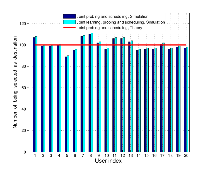
Fig. 4 illustrates the frequency of each user being scheduled in a relatively short period of 2000 slots. Each of the 20 user is selected as the destination for roughly 100 slots. That is, the scheme is fair to all users even within a small application time window.

Fig. 5 presents the probability that $k$ users have been probed until transmission. The theoretical results are from Lemma 1. The figure shows that both the Algorithm 1 and Algorithm 2 coincide with the theoretical results. We observe from the figure that the probability decreases sharply as the probing step approaches $J_{max}$ .

Fig. 6 plots the scheduling gain of the proposed algorithms versus the number of users in the system. The simulation runs for 20,000 slots. In fact the simulation result matches the analytical result of Theorem 4 quite well. Also, we note the scheduling gain remains about the same for more than 9 users. Because at this time, the cost of user probing is dominant and the scheme always tries to carry out the user probing till the end.

V-B Comparison between the Proposed Scheme and Other Schemes

The fraction of slot for probing one user is still set $\beta=0.1$ . Here four schemes are considered: (a) the proposed joint probing and scheduling scheme; (b) Round robin scheduling; (c) Genie-aided PF (GA-PF) scheme where full CQI is available to the scheduler at the beginning of each slot; (d) Probe-all PF (PA-PF) scheme where the transmitter probes all users before scheduling. For both (c) and (d), the transmitter selects the user with the largest $R_{k}(n)/T_{k}(n-1)$ for transmission. From [22] we know that the scheduling gain of GA-PF is $\mathbb{E}\left[\max\limits_{k=1,\cdots,K}X_{k}\right]$ . Then that of PA-PF is $\max(1-K\beta,0)\mathbb{E}\left[\max\limits_{k=1,\cdots,K}X_{k}\right]$ .

Fig. 7 presents the scheduling gain of schemes (a)-(d) as a function of the number of users. We can see from Fig. 7 that when probing cost is taken into account, the scheduling gain does not always increase but approaches to a limit value as the number of users increases. This indicates that, by ignoring the cost of channel probing, the ideal genie-aided PF does not reflect the correct multiuser diversity characteristics. The comparison also shows the advantage of the proposed joint probing and scheduling scheme. For the probe-all PF scheme, it achieves higher gain than round robin when the user population is not very large compared with $\beta^{-1}$ . However, when the number of user increases to some extent, the scheduling gain of probe-all algorithm vanishes. That is because almost all the period of one slot is used for user-probing instead of data transmission.

Fig. 8 displays the sum throughput of all schemes as the number of users increases. One can see that there exists a relative large gap between the ideal genie-aided PF curve and the proposed scheme. The gap quantifies the the extent to which the user probing decreases the system performance. For example, when the number of users is $K=20$ , the throughput of the joint probing and scheduling scheme only accounts for 55.64% of that of the genie-aided PF. And the throughput achieved by the joint scheme is the highest among all the non-ideal schemes (a), (b) and (d). The probe-all PF scheme performs similar to the joint probing and scheduling scheme when there are not many users ( $K\leq 6$ ), but degrades fast and even vanishes when the number of users becomes large.

VI Conclusion

We have studied the problem of achieving proportional fairness in wireless systems when explicitly taking into account the channel probing cost. An optimal adaptive joint probing and scheduling scheme is presented, as well as a static threshold based criteria for determining whether to probe or to transmit. Using the steady-state analysis, we have evaluated the scheduling gain explicitly. Extension of the scheme to the case in which the scheduler has no knowledge of the channel rate distribution has been developed, which achieves almost the same performance of the algorithm obtained under known rate statistics assumption and outperforms other non-ideal PF schemes. In this work, we have focused on the well-studied proportional fairness rule. It is possible to extend the results to more general utilities, for example, the $\alpha$ fair utility [7]. The methodology presented in this paper can then be carried through to that case as well.

Appendix A Proof of Theorem 1

Proof:

Let the largest throughput-normalized user rate after probing $j$ users be denoted by

\displaystyle w_{j}=\max_{1\leq l\leq j}s_{k^{(l)}}

(20)

Then the current reward can be written as $y_{j}(s_{k_{1}},\cdots,s_{k_{j}})=(1-j\beta)w_{j}$ and the expected reward obtained from probing the next user is

\mathbb{E}[y_{j+1}(s_{k_{1}},\cdots,s_{k_{j+1}})|s_{k_{1}},\cdots,s_{k_{j}}]=(1-(j+1)\beta)\mathbb{E}[w_{j}\vee s_{k_{j+1}}|w_{j}].

(21)

Then the event $\mathcal{E}_{j}$ can be expressed as

\mathcal{E}_{j}=\{(1-j\beta)w_{j}\geq(1-(j+1)\beta)\mathbb{E}[w_{j}\vee s_{k_{j+1}}|w_{j}]\}.

(22)

We first show that there exists a threshold $w_{j}^{(th)}$ such that the event $\mathcal{E}_{j}$ can be represented as $\mathcal{E}_{j}=\{w_{j}\geq w_{j}^{(th)}\}$ . To this end, let $f_{j}(w)=(1-j\beta)w-(1-(j+1)\beta)\mathbb{E}[w\vee s_{k_{j+1}}]$ . Then $w\in\mathcal{E}_{j}\Leftrightarrow f_{j}(w)\geq 0$ . It is easy to verify that $f_{j}(0)<0$ and $f_{j}(\infty)>0$ . The function $f_{j}(w)$ can be reorganized as $f_{j}(w)=\beta\mathbb{E}[w\vee s_{k_{j+1}}]+(1-j\beta)\mathbb{E}[w-w\vee s_{k_{j+1}}]$ . For any $w^{\prime}>w>0$ ,

f_{j}(w^{\prime})-f_{j}(w)=\beta\mathbb{E}[w^{\prime}\vee s_{k_{j+1}}-w\vee s_{k_{j+1}}]+(1-j\beta)\mathbb{E}[w^{\prime}-w+w^{\prime}\vee s_{k_{j+1}}-w\vee s_{k_{j+1}}].

Note that $w^{\prime}\vee s_{k_{j+1}}\geq w\vee s_{k_{j+1}}$ and $w^{\prime}-w\geq w^{\prime}\vee s_{k_{j+1}}-w\vee s_{k_{j+1}}$ . Thus $f_{j}(w^{\prime})-f_{j}(w)\geq 0$ , that is, $f_{j}(w)$ is a nondecreasing function. Summarizing the properties of $f_{j}(w)$ , it can be seen that the solution to $f_{j}(w)\geq 0$ can be expressed as $w\geq w_{j}^{(th)}$ .

We next show that $w_{j+1}^{(th)}\leq w_{j}^{(th)}$ . For fixed $w$ ,

	$\displaystyle f_{j+1}(w)-f_{j}(w)$
$\displaystyle=$	$\displaystyle(1-(j+1)\beta)w-(1-(j+2)\beta)\mathbb{E}_{s_{k_{j+2}}}[w\vee s_{k_{j+2}}]-(1-j\beta)w+(1-(j+1)\beta)\mathbb{E}[w\vee s_{k_{j+1}}]$
$\displaystyle=$	$\displaystyle\beta\mathbb{E}_{s_{k_{j+2}}}[w\vee s_{k_{j+2}}-w]+(1-(j+1)\beta)\{\mathbb{E}[w\vee s_{k_{j+1}}]-\mathbb{E}_{s_{k_{j+2}}}[w\vee s_{k_{j+2}}]\}$
$\displaystyle\geq$	$\displaystyle 0.$	(23)

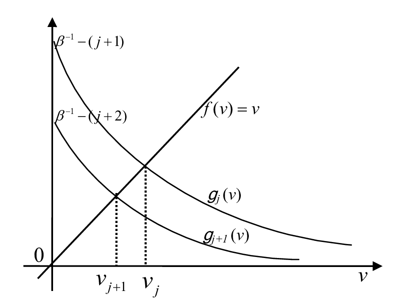
where the last ‘ $\geq$ ’ follows from the fact that $s_{k_{j+1}}$ and $s_{k_{j+2}}$ are of the same type of distribution and $\mathbb{E}s_{k_{j+1}}\geq\mathbb{E}s_{k_{j+2}}$ . Note that $w_{j}^{(th)}$ is the zero point of the function $f_{j}(w)$ . Hence $w_{j+1}^{(th)}\leq w_{j}^{(th)}$ , as illustrated in Fig. 1.

Collecting the preceding results, we have $\mathcal{E}_{j}=\{w_{j}\geq w_{j}^{(th)}\}\subseteq\{w_{j+1}\geq w_{j}^{(th)}\}\subseteq\{w_{j+1}\geq w_{j+1}^{(th)}\}=\mathcal{E}_{j+1}$ . ∎

References

[1] J. Mo and J. Walrand, “Fair end-to-end window-based congestion control,” IEEE/ACM Trans. Netw., vol. 8, no. 5, pp. 556-567, Oct. 2000.
[2] P. Viswanath, D. N. C. Tse, and R. Laroia, “Opportunistic beamforming using dumb antennas,” IEEE Trans. Inf. Theory., vol. 48, no. 6, pp. 1277-1294, June 2002.
[3] F. P. Kelly, “Charging and rate control for elastic traffic”, Euro. Trans. Telecommun., vol 8, pp. 7-20, 1997.
[4] H. J. Kushner and P. A. Whiting, “Convergence of proportional-fair sharing algorithms under general conditions”, IEEE Trans. Wireless Commun., vol. 3, no. 4. pp. 1250-1259, July 2004.
[5] S. Borst and M. Jonckheere, “Flow-level stability of channel-aware scheduling algorithms”, in Proc. WiOpt 06, 2006.
[6] J. G. Choi and S. Bahk, “Cell-throughput analysis of the proportional fair scheduler in the single-cell environment”, IEEE Trans. Veh. Technol., vol. 56, no. 2, pp. 766 - 778, 2007.
[7] J. Liu, A. Proutiere, Y. Yi, M. Chiang and H. V. Poor, “Stability, fairness, and performance: A flow-level study on nonconvex and time-varying rate regions”, IEEE Trans. Inf. Theory., vol. 55, no. 8, pp. 3437 - 3456, 2009.
[8] C. W. Chan and N. Bambos, “Throughput loss in task scheduling due to server state uncertainty,” VALUETOOLS 2009.
[9] S. Guha, K. Mungala, and S. Sarkar, “Jointly optimal transmission and probing strategies for multichannel wireless systems”, In CISS 06, Mar 2006.
[10] N. Chang and M. Liu. “Optimal channel probing and transmission scheduling for opportunistic spectrum access,” In ACM MOBICOM, 2007.
[11] P. Chaporkar and A. Proutiere, “Optimal joint probing and transmission strategy for maximizing throughput in wireless systems,” IEEE Journal on Selected Areas in Communications, vol. 26, no.8, pp. 1546-1556, 2008.
[12] J. Chen, R. A. Berry, and M. L. Honig, “An adaptive limited feedback scheme for MIMO OFDM based on optimal stopping”, Proc. Allerton Conference, 2008.
[13] A. Gopalan, C. Caramanis and S. Shakkotai, “On wireless scheduling with partial channel-state information,” in Allerton Conference on Communication, Control, and Computing, 2007.
[14] M. Ouyang and L. Ying, “On scheduling in multi-channel wireless downlink networks with limited feedback”, In Proc. Allerton Conference, 2009.
[15] P. Chaporkar, A. Proutiere, H. Asnani and A. Karandikar, “Scheduling with limited information in wireless systems”, in ACM MobiHoc, 2009.
[16] H. Zhou, P. Fan and D. Guo, “The Impact of Limited Information on Proportional Fair Scheduling In Wireless Networks”, accepted by IEEE GLOBECOM 2010.
[17] A. L. Stolyar, “On the asymptotic optimality of the gradient scheduling algorithm for multiuser throughput allocation”, Opreations Research, vol. 53, no. 1, January-February 2005, pp. 12-25.
[18] T. Ferguson, “Optimal stopping and applications,” [Online]. Available: http://www.math.ucla.edu/~tom/Stopping/Contents.html, 2006.
[19] V. S. Borkar, Stochastic Approximation: A Dynamical Systems Viewpoint. Cambridge University Press, 2008.
[20] D. A. Berry and B. Fristedt, Bandit Problems: Sequential Allocation of Experiments, London: Chapman and Hall, 1985.
[21] R. Agrawal, “Sample mean based index policies with O(log n) regret for the multi-armed bandit problem,” Advances in Applied Probability, Vol. 27, No. 4, pp. 1054-1078, 1995.
[22] S. Borst, “User level aware performance of channel-aware scheduling algorithms in wireless data networks,” in Proc. Infocom, 2002.

Refer to caption — Fig. 1: Illustration of the property of function $f_{j}(w)$ .