Maximizing the Total Resolution of Graphs
Abstract
A major factor affecting the readability of a graph drawing is its resolution. In the graph drawing literature, the resolution of a drawing is either measured based on the angles formed by consecutive edges incident to a common node (angular resolution) or by the angles formed at edge crossings (crossing resolution). In this paper, we evaluate both by introducing the notion of “total resolution”, that is, the minimum of the angular and crossing resolution. To the best of our knowledge, this is the first time where the problem of maximizing the total resolution of a drawing is studied.
The main contribution of the paper consists of drawings of
asymptotically optimal total resolution for complete graphs
(circular drawings) and for complete bipartite graphs (-layered
drawings). In addition, we present and experimentally evaluate a
force-directed based algorithm that constructs drawings of large
total resolution.
Date: September 10, 2010.
1 Introduction
Graphs are widely used to depict relations between objects. There exist several criteria that have been used to judge the quality of a graph drawing [3, 16]. From a human point of view, it is necessary to obtain drawings that are easy-to-read, i.e., they should nicely convey the structure of the objects and their relationships. From an algorithmic point of view, the quality of a drawing is usually evaluated by some objective function and the main task is to determine a drawing that minimizes or maximizes the specific objective function. Various such functions have been studied by the graph drawing community, among them, the number of crossings among pairs of edges, the number of edge bends, the maximum edge length, the total area occupied by the drawing and so on.
Over the last few decades, much research effort has been devoted to the problem of reducing the number of crossings. This is reasonable, since it is commonly accepted that edge crossings may negatively affect the quality of a drawing. Towards this direction, there also exist eye-tracking experiments that confirm the negative impact of edge crossings on the human understanding of a graph drawing [20, 21, 22]. However, the computational complexity of the edge crossing minimization problem, which is -complete in general [11], implies that the computation of high-quality drawings of dense graph is difficult to achieve.
Apart from the edge crossings, another undesired property that may negatively influence the readability of a drawing is the presence of edges that are too close to each other, especially if these edges are adjacent. Thus, maximizing the angles among incident edges becomes an important aesthetic criterion, since there is some correlation between the involved angles and the visual distinctiveness of the edges.
Motivated by the cognitive experiments by Huang et al. [14, 15] that indicate that the negative impact of an edge crossing is eliminated in the case where the crossing angle is greater than degrees, we study a new graph drawing scenario in which both angular and crossing resolution11 1 The term angular resolution denotes the smallest angle formed by two adjacent edges incident to a common node, whereas the term crossing resolution refers to the smallest angle formed by a pair of crossing edges. are taken into account in order to produce a straight-line drawing of a given graph. To the best of our knowledge, this is the first attempt, where both angular and crossing resolution are combined to produce drawings. We prove that the classes of complete and complete bipartite graphs admit drawings that asymptotically maximize the minimum of the angular and crossing resolution (Section 3). We also present a more practical, force-directed based algorithm that constructs drawings of large angular and crossing resolution (Section 4).
1.1 Previous Work
Formann et al. [9] were the first to study the angular resolution of straight-line drawings. They proved that deciding whether a graph of maximum degree admits a drawing of angular resolution (i.e., the obvious upper bound) is -hard. They also proved that several types of graphs of maximum degree have angular resolution . Malitz and Papakostas [18] proved that any planar graph of maximum degree , admits a planar straight-line drawing with angular resolution . Garg and Tamassia [12] showed a continuous tradeoff between the area and the angular resolution of planar straight-line drawings. Gutwenger and Mutzel [13] gave a linear time and space algorithm that constructs a planar polyline grid drawing of a connected planar graph with vertices and maximum degree on a grid with at most bends and minimum angle greater than . Bodlaender and Tel [2] showed that planar graphs with angular resolution at least are rectilinear. Recently, Lin and Yen [17] presented a force-directed method based on edge-edge repulsion that leads to drawings with high angular resolution. In their work, pairs of edges incident to a common node are modeled as charged springs, that repel each other.
A graph is called right angle crossing (or RAC for short) graph if it admits a polyline drawing in which every pair of crossing edges intersects at right angle. Didimo et al. [6] showed that any straight-line RAC drawing with nodes has at most edges. Angelini et al. [1] showed that there are acyclic planar digraphs not admitting straight-line upward RAC drawings and that the corresponding decision problem is -hard. They also constructed digraphs whose straight-line upward RAC drawings require exponential area. Di Giacomo et al. [5] presented tradeoffs between the crossing resolution, the maximum number of bends per edges and the area. Dujmovic et al. [7] studied Angle Crossing (or AC for short) graphs, that generalize the RAC graphs. A graph is called AC if it admits a polyline drawing in which the smallest angle formed by an edge crossing is at least . For this class of graphs, they proved upper and lower bounds for the number of edges.
Force-directed methods are commonly used for drawing graphs [8, 10]. In such a framework, a graph is treated as a physical system with forces acting on it. Then, a good configuration or drawing can be obtained from an equilibrium state of the system. An overview of force-directed methods and their variations can be found in the graph drawing books [3, 16].
2 Preliminaries and Notation
Let be an undirected graph. Given a drawing of , we denote by the position of node on the plane. The unit length vector from to is denoted, by , where . The degree of node is denoted by . Let also be the degree of the graph.
Given a pair of points , with a slight abuse of notation, we denote by the Euclidean distance between and . We refer to the line segment defined by and as .
Let and be two vectors. The vector which bisects the angle between and is . We denote by the corresponding unit length vector. Given a vector , we refer to the unit length vector which is perpendicular to and precedes it in the clockwise direction, as . Some of our proofs use the following elementary geometric properties:
| (1) |
| (2) |
| (3) |
3 Drawings with Optimal Total Resolution for Complete and Complete Bipartite Graphs
In this section, we define the total resolution of a drawing and we present drawings of asymptotically optimal total resolution for complete graphs (circular drawings) and complete bipartite graphs (-layered drawings).
Definition 1
The total resolution of a drawing is defined as the minimum of its angular and crossing resolution.
We first consider the case of complete graphs. Let be a complete graph, where and . Our aim is to construct a circular drawing of of maximum total resolution. Our approach is constructive and common when dealing with complete graphs. A similar one has been given by Formann et al. [9] for obtaining optimal drawings of complete graphs, in terms of angular resolution. Consider a circle of radius centered at and circumscribe a regular -polygon on . In our construction, the nodes of coincide with the vertices of . W.l.o.g., we further assume that appear in this order in the counter-clockwise direction around , as illustrated in Fig.1a.
Theorem 3.1
A complete graph admits a drawing of total resolution .
Proof
We prove that the angular resolution of the presented drawing of is , whereas its crossing resolution is . First, observe that the arc of circle that connects two consecutive nodes and is equal to , for each . Therefore, the angular resolution of the drawing is , as desired. Let now and be two crossing edges. Without loss of generality, we assume that , as in Fig.1a. The crossing of and defines two angles and such that . In Fig.1a, is exterior to the triangle formed by the crossing of and and the nodes and (refer to the dark-gray triangle of Fig.1a). Therefore: . Similarly, . In the case, where and (i.e., the nodes (, resp.) and (, resp.) are consecutive), the angle receives its minimum value, which is equal to . Similarly, we can prove that the minimum value of is also . This establishes that the crossing resolution is .∎
We now proceed to consider the class of complete bipartite graphs. Since an -vertex complete bipartite graph is a subgraph of a -vertex complete graph, the bound of the total resolution of a complete bipartite graph can be implied by the bound of the complete graph. However, if the nodes of the graph must have integer coordinates, i.e., we restrict ourselves on grid drawings, few results are known regarding the area needed of such a drawing. An upper bound of area can be implied by [2]. This motivates us to separately study the class of complete bipartite graph, since we can drastically improve this bound. Note that the tradeoff between resolution and area has been studied by the graph drawing community, in the past. Malitz and Papakostas [18] showed there exist graphs that always require exponential area for straight-line embeddings maintaining good angular resolution. The claim remains true, if circular arc edges are used instead of straight-line [4]. More recently, Angelini et al. [1] constructively showed that there exists graphs whose straight-line upward RAC drawings require exponential area.
Again, we follow a constructive approach. First, we consider a square where its top and bottom sides coincide with and , respectively (see Fig.1b). Let be the height (and width) of . According to our approach, the nodes of (, resp.) reside along side (, resp.) of . In order to specify the exact positions of the nodes along side , we first construct a bundle of semi-lines, say , each of which emanates from vertex and crosses side of , so that the angle formed by and semi-line equals to , for each . These semi-lines split angle into angles, each of which is equal to , since . Say . Then, we place node at the intersection of semi-line and , for each (see Fig.1b). In order to simplify the description of our approach, we denote by the horizontal distance between two consecutive nodes and , .
We proceed by defining an additional bundle of semi-lines, say , that emanate from vertex . More precisely, semi-line emanates from vertex and passes through the intersection of and (i.e., node ), for each (see Fig.1b). Let be the angle formed by two consecutive semi-lines and , for each .


So far, we have managed to fix the position of the nodes of only (along side of ). Symmetrically, we define the position of the nodes of along side of . This only involves two additional bundles of semi-lines emanating from vertices and . We now proceed to investigate some geometric properties of the proposed construction.
Lemma 1
For each , it holds that .
Proof
By induction. For the base of the induction, we have to show that . First observe that and . Therefore:
However, both and are greater than zero, which immediately implies that . For the induction hypothesis, we assume that , it holds that and we should prove that . Obviously, . Based on Equation 1 and similarly to the base of the induction, we have:
- •
- •
In order to complete the proof, observe that .∎
Lemma 2
For each , it holds that .
Proof
By induction. For the base of the induction, we have to prove that or equivalently that . It holds that and . By combining these relationships with Equation 1 we have that . Therefore:
which trivially holds due to Lemma 1. For the induction hypothesis, we assume that , it holds that and we have to show that . Observe that:
- •
=
- •
By Lemma 1 we have that and . Therefore, .∎
Lemma 3
Angle is the smallest angle among all the angles formed in the drawing.
Proof
From Lemma 2, it follows that angle is the smallest angle among all , . Additionally, it is not difficult to see that angle is larger (but remains the smallest among all , ), if the endpoint of the bundle (i.e., node ) moves to any internal point (i.e., node ) of side (see Fig.1b). Therefore, is the smallest angle among all the angles formed by pairs of consecutive edges incident to any node of . Since , the same holds for the nodes of . Therefore, defines the angular resolution of the drawing.
Consider now two crossing edges (refer to the bold, crossing dashed-edges of Fig.1b). Their crossing defines (a) a pair of angles that are smaller than and (b) another pair of angles that are larger than . Obviously, only the acute angles participate in the computation of the crossing resolution (see angle in Fig.1b). However, in a complete bipartite graph the acute angles are always exterior to a triangle having two of its vertices on and , respectively (refer to the gray-colored triangle of Fig.1b). Therefore, the crossing resolution is always greater than the angular resolution, as desired. ∎
Lemma 4
It holds that .
Proof
We equivalently prove that . Using Equation 2, we have that . Therefore:
which obviously holds.∎
Theorem 3.2
A complete bipartite graph admits a -layered drawing of total resolution .
Consider now the case where the nodes of the graph must have integer coordinates, i.e., we restrict ourselves on grid drawings. An interesting problem that arises in this case is the estimation of the total area occupied by the produced drawing. We will describe how we can modify the positions of the nodes produced by our algorithm in order to obey the grid constraints. Assume without loss of generality that and are two horizontal lines, so that coincides with -axis and the drawing produced by our algorithm has . Then, we can express the height of drawing as a function of , as follows:
Note that this drawing does not obey the grid constraints. To achieve this, we move the horizontal line to the horizontal grid line immediately above it and each node of both and to the rightmost grid-point to its left. In this manner, we obtain a new drawing , which is grid as desired. By Lemma 1, it follows that there are no two nodes sharing the same grid point, since is slightly greater than one grid unit. Since neither horizontal line nor any node of moves more than one unit of length, the total resolution of is not asymptotically affected, and, in addition the height of the drawing is not significantly greater (i.e., asymptotically it remains the same). Based on the above, the area is bounded by or equivalently by . By Equation 3, this is further bounded by . By Theorem 3.2, it holds that . Therefore, the total area occupied by the drawing is . The following theorem summarizes this result.
Theorem 3.3
A complete bipartite graph admits a -layered grid drawing of total resolution and area.
4 A Force Directed Algorithm
We present a force-directed algorithm that given a reasonably nice initial drawing, probably produced by a classical force-directed algorithm, results in a drawing of high total resolution. The algorithm reinforces the classical force-directed algorithm of Eades [8] with some additional forces exerted to the nodes of the graph. More precisely, these additional forces involve springs and some extra attractive or repulsive forces on nodes with degree greater than one and on end-nodes of edges that are involved in an edge crossing. This aims to ensure that the angles between incident edges and the angles formed by pairs of crossing edges will be as large as possible. The classical force-directed algorithm of Eades [8] models the nodes of the graph as electrically charged particles that repel each other, and its edges by springs in order to attract adjacent nodes. In our approach, we use only the attractive forces of the force-directed algorithm of Eades (denoted by ), which follow the formula:
where and capture the stiffness and the natural length of the springs, respectively. Recall that denotes the unit length vector from to .
We first describe our approach for the case where two edges, say and , are involved in a crossing. Let be their intersection point. W.l.o.g., we assume that and are to the left of and , respectively, and , as in Fig.2. Let be the angle formed by the line segments and in counter-clockwise order around from to . In order to avoid confusion, we assume that , i.e., we abuse the counter-clockwise measurement of the angles that would result in . Similarly, we define the remaining angles of Fig.2. Obviously, . Ideally, we would like , i.e., and form a right angle crossing. As we will shortly see, the magnitude of the forces that we apply on the nodes and depends on (a) the angles and and (b) the lengths of the line segments , , and .
The physical model that describes our approach is illustrated in Fig.2. Initially, for each pair of crossing edges at point , we place springs connecting consecutive nodes in the counter-clockwise order around , as in Fig.2a. The magnitude of the forces due to these springs should capture our preference for right angles. Consider the spring connecting and . The remaining ones are treated symmetrically. We set the natural length, say , of the spring connecting the nodes and to be . This quantity corresponds to the length of the line segment that connects and in the optimal case where . So, in an equilibrium state of this model on a graph consisting only of and , and will form a right angle. Concluding, the force on due to the spring of is defined as follows:


The remaining forces of Fig.2a are defined similarly. Note that in the formula above, the constant is used to control the stiffness of the springs.
Our preference for right angle crossings can be also captured using the angles and (see Fig.2b). As in the previous case, we restrict our description on the angle formed by the line segments and . Ideally, we would like to exert forces on the nodes and such that: (i) when , the magnitude of the force is very large (in order to repel and ), and (ii) when , the magnitude of the force is very small. A function, say , which captures this property is: . Having specified the magnitude of the forces, we set the direction of the force on (due to ) to be perpendicular to the line that bisects the angle (refer to the dash-dotted line of Fig.2b), or equivalently parallel to the unit length vector . Recall that and refer to the perpendicular and bisector vectors, respectively (see Section 2). It is clear that if , the forces on and should be repulsive (in order to enlarge the angle between them), otherwise attractive. This can be captured by the function. We conclude with the following formula which expresses the force on due to .
where constant controls the strength of the force. Similarly, we define the remaining forces of Fig.2b.
Consider now a node
that is incident to edges, say ,
, , . We assume that
are consecutive in the counter-clockwise
order around in the drawing of the graph (see
Fig.3a). Similarly to the case of
two crossing edges, we proceed to connect the endpoints of consecutive edges around
by springs, as in Fig.3a. In
this case, the natural length of each spring, should capture our
preference for angles equal to .
In order to achieve this, we proceed as follows: For each
, we set the natural length, say
, of the spring connecting with
, to be:
where is used to denote the length of the edge
in the drawing of the graph. The quantity
corresponds to the length of the line segment
that connects with in the optimal case
where the angle formed by and is
.
Therefore, the spring forces between consecutive edges should follow
the formula:
where the quantity is a constant which captures the stiffness of the spring.


Let now be the angle formed by and , measured in counter-clockwise direction from to , . Similarly to the case of two crossing edges, we exert forces on and perpendicular to the bisector of , as illustrated in Fig.3b. However, in this case we need a magnitude function such that: (i) when , the magnitude of the force is very large (in order to repel and ), and (ii) when , the magnitude of the force is very small. Such a function, say , is: . Having fully specified the forces applied on the endpoints of consecutive edges and their directions, we are now ready to provide the exact formulas that the forces follow:
where is a constant to control the strength of the force. In the work of Lin and Yen [17], the above technique which applies large repelling forces perpendicular to the bisector of the angle, when the angle is small, is referred to as edge-edge repulsion. However, in their work, they use different metric to control the magnitude function. Of course, we could also use their metric, but we prefer the one reported above in order to maintain a uniform approach in both crossing and angular cases. In Section 4.1, we provide an experimental comparison of these techniques.
Note that by setting zero values to the constants , or , , our algorithm can be configured to maximize the angular, or the crossing resolution only, respectively.
On each iteration, our algorithm computes three types of forces. Computing the attractive forces of the classical force-directed model among pairs of adjacent nodes of the graph requires time per iteration. The computation of the forces due to the edge crossings needs time, assuming a straight forward algorithm that in time reports all pairwise crossing edges. Finally, the computation of the forces due to the angles between consecutive edges can be done in time per iteration, where denotes the degree of the graph, since we first sort the incident edges of each node of the graph in cyclic order. Summarizing the above, each iteration of our algorithm takes time.
The time complexity can be improved using standard techniques from computational geometry [19]. If is the number of pairwise-crossing edges, then the intersections can be reported in time [19, pp.277], which leads to a total complexity per iteration.
4.1 Experimental Results
In this section, we present the results of the experimental evaluation of our algorithm. Apart from our algorithm, we have implemented the force directed algorithms of Eades [8] and Lin and Yen [17]. The implementations are in Java using the yFiles library (http://www.yworks.com). The experiment was performed on a Linux machine with 2.00 GHz CPU and 2GB RAM using the Rome graphs (a collection of around 11.500 graphs) obtained from graphdrawing.org. Fig.4, illustrates a drawing of a Rome graph with nodes and edges produced by our force directed algorithm.

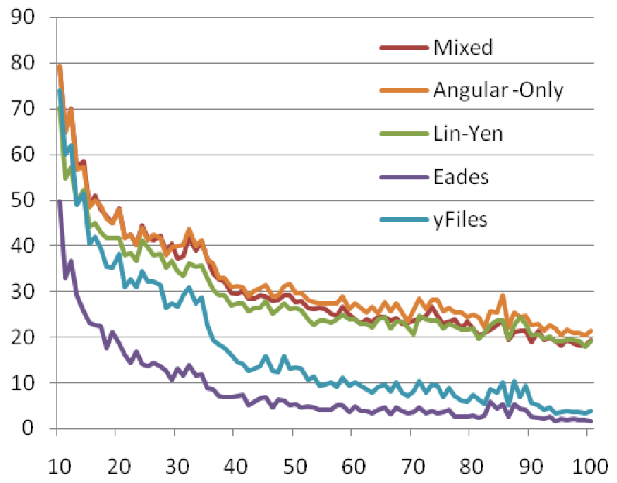
The experiment was performed as follows. First, each Rome graph was laid out using the SmartOrganic layouter of yFiles. This layout was the input layout for all three algorithms, in order to speed up the experiment and overcome problems associated with local minimal traps especially in large graphs. If both the angular and the crossing resolution between two consecutive iterations of each algorithm were not improved more that 0.001 degrees, we assumed that the algorithm has converged and we did not proceed any more. The maximum number of iterations that an algorithm could perform in order to converge was 100.000. We note that the termination condition is quite strict and demands a large number of iterations. Our algorithm is evaluated as (a) Crossing-Only, (b) Angular-Only and (c) Mixed. The results are illustrated in Fig.5 and should be viewed in color.
The Angular Resolution Maximization Problem: Refer to Fig.5a. Our experimental analysis shows that our Angular-Only algorithm achieves, on average, better angular resolution. The angular resolution of our Mixed algorithm is almost equal, on average, to the one of Lin and Yen. Note that the algorithm of Lin and Yen, in contrast to ours, does not modify the embedding of the initial layout [17] (i.e., it needs a close-to-final starting layout and improve on it). This explains why our Mixed algorithm achieves almost the same performance, in terms of angular resolution, as the one of Lin and Yen. In % of the graphs our Mixed algorithm yields a better solution compared to Lin-Yen’s algorithm with an average improvement of .
The Crossing Resolution Maximization Problem: In Fig.5b the data were filtered to depict only the results of non-planar drawings produced by the algorithms and avoid infinity values in the case of planar ones. It is clear that our Crossing-Only algorithm results in drawings with high crossing resolution. Our Crossing-Only algorithm performs better on large graphs compared to the algorithm of yFiles. The average improvement implied by our Crossing-Only algorithm is w.r.t. the yFiles algorithm.
The Total Resolution Maximization Problem: Refer to Fig.5c. This is the most important result of our experimental analysis. It indicates that our Mixed algorithm applied on graphs with more than nodes constructs drawings with total resolution of degrees, on average. Note that this is an achievement on average and under the particular termination condition discussed above, i.e., there is no guarantee, that it would be maintained indefinitely. An example is given in Fig.4.
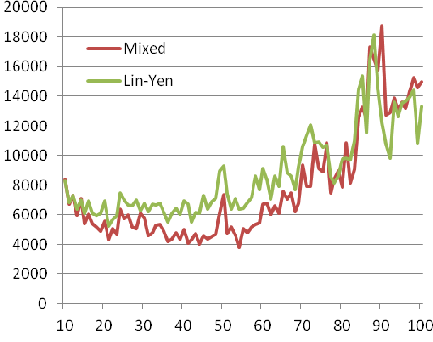
Finally, Fig.5d summarizes the running time performance of the algorithms. Our algorithm needs, on average, milliseconds and iterations to converge, whereas the one of Lin and Yen and , respectively. Note that the time complexity of Lin-Yen’s algorithm is better than ours. However, the termination condition takes into account the crossing improvement and therefore the algorithm of Lin and Yen needs more iterations to converge, which explains this contradiction.


5 Conclusions
In this paper, we introduced and studied the total resolution maximization problem. Of course, our work leaves several open problems. It would be interesting to try to identify other classes of graphs that admit optimal drawings. Even the case of planar graphs is of interest, as by allowing some edges to cross (say at large angles), we may improve the angular resolution and therefore the total resolution.
References
- [1] P. Angelini, L. Cittadini, G. Di Battista, W. Didimo, F. Frati, M. Kaufmann, and A. Symvonis. On the perspectives opened by right angle crossing drawings. In Proc. of 17th Int. Symp. on Graph Drawing (GD 2009), 2009.
- [2] I. Bárány and N. Tokushige. The minimum area of convex lattice n-gons. Combinatorica, 24(2):171–185, 2004.
- [3] G. D. Battista, P. Eades, R. Tamassia, and I. G. Tollis. Algorithms for drawing graphs: an annotated bibliography. Comput. Geom., 4:235–282, 1994.
- [4] C. C. Cheng, C. A. Duncanyz, M. T. Goodrichz, and S. G. Kobourovz. Drawing planar graphs with circular arcs. Discrete and Computational Geometry, 25:117–126, 1999.
- [5] E. Di Giacomo, W. Didimo, G. Liotta, and H. Meijer. Area, curve complexity, and crossing resolution of non-planar graph drawings. In Proc. of 17th Int. Symp. on Graph Drawing (GD 2009), 2009.
- [6] W. Didimo, P. Eades, and G. Liotta. Drawing graphs with right angle crossings. In Proc. of the Algorithm and Data Structure Symp. (WADS 2009), 2009.
- [7] V. Dujmovic, J. Gudmundsson, P. Morin, and T. Wolle. Notes on large angle crossing graphs. In Computing: Theory of Computing 2010. Australian Computer Society, 2010.
- [8] P. Eades. A heuristic for graph drawing. Congressus Numerantium, (42):149–160, 1984.
- [9] M. Formann, T. Hagerup, J. Haralambides, M. Kaufmann, F. Leighton, A. Symvonis, E. Welzl, and G. Woeginger. Drawing graphs in the plane with high resolution. SIAM J. Comput., 22(5):1035–1052, 1993.
- [10] T. Fruchterman and E. M. Reingold. Graph drawing by force-directed placement. Software-Practice and Experience, 21(11):1129–1164, 1991.
- [11] M. Garey and D. Johnson. Crossing number is np-complete. SIAM J. Algebraic Discrete Methods, 4:312–316, 1983.
- [12] A. Garg and R. Tamassia. Planar drawings and angular resolution: Algorithms and bounds (extended abstract). In Proc. 2nd Annu. Eur. Sympos. Alg., pages 12–23, 1994.
- [13] C. Gutwenger and P. Mutzel. Planar polyline drawings with good angular resolution. In Proc. of 6th Int. Symp. on Graph Drawing, volume 1547 of LNCS, pages 167–182, 1998.
- [14] W. Huang. Using eye tracking to investigate graph layout effects. Asia-Pacific Symp. on Visualization, pages 97–100, 2007.
- [15] W. Huang, S.-H. Hong, and P. Eades. Effects of crossing angles. In PacificVis, pages 41–46, 2008.
- [16] M. Kaufmann and D. Wagner, editors. Drawing Graphs: Methods and Models, volume 2025 of LNCS. Springer-Verlag, 2001.
- [17] C.-C. Lin and H.-C. Yen. A new force-directed graph drawing method based on edge-edge repulsion. In Proc. of the 9th Int. Conf. on Inf. Vis., pages 329–334. IEEE, 2005.
- [18] S. M. Malitz and A. Papakostas. On the angular resolution of planar graphs. In STOC, pages 527–538, 1992.
- [19] F. P. Preparata and M. I. Shamos. Computational geometry: an introduction. Springer-Verlag, 1985.
- [20] H. C. Purchase. Effective information visualisation: a study of graph drawing aesthetics and algorithms. Interacting with Computers, 13(2):147–162, 2000.
- [21] H. C. Purchase, D. A. Carrington, and J.-A. Allder. Empirical evaluation of aesthetics-based graph layout. Empirical Software Engineering, 7(3):233–255, 2002.
- [22] C. Ware, H. Purchase, L. Colpoys, and M. McGill. Cognitive measurements of graph aesthetics. Information Visualization, 1(2):103–110, 2002.