Inertial Josephson Relation for FIR Frequencies
Abstract
Consideration of the balance of forces on superconducting condensate at low frequencies leads to the well-known Josephson Relation. Using the Ginzburg-Landau expression for the current, an expression relating the electric field to the vortex velocity via the magnetic field is obtained. This result is the Josephson Relation, supplemented by a term accounting for the inertia of charge carriers. This Inertial Josephson Relation may be used at all frequencies and may be viewed as the Josephson Relation extended to the case of sub-gap high-frequency response. When applied to vortex dynamics it yields the same conductivity as solution of the Ginzburg-Landau theory.
Keywords:
non-equilibrium superconductivity; time-dependent Ginzburg-Landau theorypacs
PACS numberVortices in the superconducting condensate are stable objects, which interact to form vortex matter [1, 2]. The response of vortex matter may be studied at various frequencies. One potential practical application of vortex matter is as a memory device; one might imagine that data could be encoded in the positioning of vortices. To attain this degree of control over vortex matter, it must be clear theoretically how forces and fields interact with vortices at the desirable high frequencies of such a putative memory device.
Low-frequency vortex motion can be observed by magnetic scanning [3], but high frequencies are invisible via this method. Fortunately, in far infra-red (FIR) spectroscopy it has been possible to make high-frequency observations of the electric current to which the vortex velocity responds [4]. Although these data have then been interpreted using the Josephson Relation [5], one may ask whether this is legitimate at high frequencies.
An alternative way to interpret the FIR data is based on the Time-Dependent Ginzburg-Landau (TDGL) theory [6, 7]. These two approaches lead to contradictory results; there is a difference in phases which is illustrated schematically in Fig. 1. Actual experimental data is shown in Fig. 2. Both approaches can reproduce the experimentally established frequency-dependent phase difference between the electric field and the current, but they yield different vortex velocities. According to the Josephson Relation
| (1) |
the vortex velocity is in phase with the electric field . In contrary, in the solution [7] of the TDGL equation derived near the transition line, the vortex velocity is in phase with the current.

These different phases of the vortex velocity lead to different interpretations of the experimental data. The motion of vortices is given by the balance of forces (per unit length)
| (2) |
where the left-hand side includes the Lorentz force due to the mean current and the pinning force proportional to the vortex displacement , and the right hand side is a friction force. Identification of these forces corresponds to the Gittleman and Rosenblum (GR) model [4] which is sufficient for our discussion. Using the Josephson Relation (1) one must interpret the experimentally observed phase difference between the field and current as a manifestation of the pinning force, . Interpreting this same case using the TDGL theory, one would not require the addition of a pinning potential.
The goal of the present paper is to show that the descrepancy discussed above is actually a consequence of the inapplicability of the Josephson Relation at high frequencies. Using the current from the GL theory, we will show how one can derive the Inertial Josephson Relation, which is similar to the Josephson Relation except for a term important only at high frequencies, which is proportional to the acceleration of charge carriers. The Inertial Josephson Relation has in fact been known in the literature for some time [8, 9], but has been derived by much less direct means than that which we propose here [8]. In [8, 9] it is motivated by the application of hydrodynamics to the superfluid state [10].
Although our arguments are in many respects more widely applicable, for the sake of simplicity we restrict our attention to a two-dimensional sample with perpendicular magnetic field creating the triangular Abrikosov vortex lattice. We will derive the relation for an ideal sample with no pinning centers. Electrons are driven by a FIR light which we represent by a homogeneous electric field parallel to the sample . The sample is of infinitesimal thickness, therefore currents in the sample have negligible feedback effect on the electromagnetic fields acting on the sample. We neglect contributions important for the Faraday rotation or the Hall voltage. Finally, we work in the vector gauge with zero scalar potential, allowing us to avoid a distracting discussion of the electrostatic and electrochemical potentials.
In principle one must solve for the order parameter from the TDGL equation
| (3) |
and then evaluate the current
| (4) |
In the limiting case of linear response these two equations can be mapped to equations (2) and (1), respectively. As shown in [11], the TDGL equation (3) implies the balance of forces on vortices (2) with . A second independent equation must be derived from the current formula (4). The electric field appears in the time derivative of the current, since .
In the linear approximation the vortex lattice is undistorted, and the order parameter reflects this as a function of time. We denote by the order parameter in the equilibrium and by its time-dependent value driven by the light. The coherent movement of the vortex lattice implies , where is a displacement of the vortex lattice at time from its equilibrium position. The phase factor is given by the relative position of the displaced vortex lattice and the center of the vector gauge, . Here is the elementary flux. When calculating , the time derivative can thus be written in terms of space derivatives; , where we have used and assumed parallel to . We find
| (5) | |||||
The transport current is the mean value obtained by averaging over the elementary cell of the lattice. We thus average the time derivative of the current (5) and express the mean current via the Cooper pair velocity, . Here is the mean density of Cooper pairs.
| (6) | |||||
Simplifying,
| (7) | |||||
The total derivative of the current is zero under integration, since the current itself is periodic on the lattice. Using the identity we thus obtain the relation
| (8) |
which is the Inertial Josephson Relation; we view it as extending the validity of the Josephson Relation (1) into the FIR region.
In Kopnin [11] is given a derivation of the Josephson Relation (1) under certain rather broad assumptions. It is useful at this stage to make contact with this well-known result, and show how this is commensurate with the Inertial Josephson Relation (8). Differences between [11] and the present paper include Kopnin’s use of gauge-invariant quantities, lack of assumption of homogeneous electric field, and use of the phase of the order parameter explicitly in his equations. None of these differences is significant in the present context. We choose to make a certain choice of gauge, but the final result is one between physical quantities. The simplicity of our calculation is increased slightly due to our assumption of a homogeneous electric field, since we may take outside when calculating the averaged current . Kopnin uses the field, which is subject to nonanalytic behaviour due to a coordinate singularity when , but this is done carefully and no descrepancy is to be found; we use the complex order parameter itself, which is not singular.
The essential difference is as follows. Kopnin assumes the vortex configuration to move coherently at constant velocity, so that in the notation of [11] (except that there is used in place of ), the vector potential is taken to be and the order parameter where and are taken to be small corrections. No compensating gauge transformation is needed here as the calculation is not performed in a particular gauge. In fact, in the time-dependent case these would need to be modified to read
| (9) |
and
| (10) |
In addition, the longitudinal part of may not be neglected, and we must insert the current
| (11) |
With these modifications, relaxing the assumption of constant-velocity motion of the vortices, the derivation of Kopnin reproduces precisely the Inertial Josephson Relation (8).
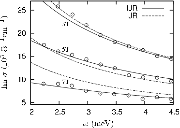
Let us illustrate in experimental context how the Inertial Josephson Relation (8) leads to conclusions different from those based on the Josephson relation (1). In Fig. 2 is shown the imaginary part of conductivity observed with Fast FIR Transmission Spectroscopy by Ikebe et al [12]. With the complex conductivity is defined by . In the GR model, balancing forces as in (2) and using the Josephson Relation (1) to interpret the experimental data, one concludes that and there obtains an imaginary part to the conductivity. From the TDGL point of view, again using (2) but with the Inertial Josephson Relation (8), one obtains a complex conductivity without recourse to postulating a pinning potential.
While excellent experimental agreement has been attained through more empirical methods such as the interpolation between normal and superconducting states of Coffey and Clem [13], we would like to stress that our derivation of the IJR relies only on the same basic physical principles as the Josephson Relation.
Using , we substitute the vortex velocity from (2) into the Josephson Relation (1), which yields
| (12) |
Since the magnetic field is perpendicular to the current, the double vector product becomes . The conductivity
| (13) |
has non-zero imaginary part exclusively due to the pinning; . As one can see in Fig. 2, this model allows for a qualitatively good fit of experimental data since the imaginary part decreases as and increases with decreasing magnetic field.
Now let us turn to the application of the Inertial Josephson Relation (8) and show that the inertial term leads to complex conductivity even in absence of pinning. We evaluate the vortex velocity from the balance equation (2) with and substitute it into the Inertial Josephson Relation (8). The resulting electric field is giving a conductivity of the Drude type
| (14) |
where is the upper critical field at zero temperature and is the relaxation time of the condensate.
In Fig. 2 we compare the imaginary part of conductivity (14) with experimental data of Ikebe et al [12] using the relaxation time in the dirty limit [11]. The experimentally established normal conductivity is and the upper critical field T, as in [12].
The GL parameter is , usual for NbN. From we find the friction coefficient . We have used the London penetration depth at zero temperature , the GL coherence length , and . The density of Cooper pairs we evaluate from the TDGL solution in the small signal limit; with the Abrikosov coefficient for the triangular lattice. Using we obtain . A good agreement of the conductivity (14) with experimental data shows that the set of equations (2) and (8) captures the FIR response without any need for the addition of pinning to the theory.
Let us revisit Josephson’s derivation of relation (1) in light of the present discussion. Josephson assumed a steady motion of vortices and condensate. Since the condensate is not permanently accelerated by passing vortices, he concluded that the electromotive force is balanced by a gradient of the electrochemical potential. Josephson’s relation (1) represents the balance of these two forces. Away from low frequencies, it becomes important that the condensate is continually accelerated by the alternating field. The balance of forces then leads to the Inertial Josephson Relation (8). Finally it is important to note, as did Josephson, that the appearing in his relation is not exactly the electric field appearing in the present paper; the subtle difference is that Josephson’s depends on the chemical potential rather than the electromagnetic scalar potential.
The derivation here is restricted to the case of an infinitesimally thin layer. It is reasonable to expect that its validity is more general, although the above analysis benefits from the simplicity of averaging over the uniform electric and magnetic field configuration. We did not consider the conductivity contribution of normal electrons; since the imaginary part of the normal conductivity is negligible, this is not important for our discussion.
We have made use of Ginzburg-Landau theory to provide a careful derivation of the Inertial Josephson Relation, which relates electric and magnetic fields to not only vortex velocity, as in the Josephson Relation, but also to the acceleration of the charge carriers. We have shown that the same reasoning which leads to the Josephson Relation at low frequencies can be used to carefully derive the more generally applicable inertial version, first suggested by Abrikosov et al [9].
We have illustrated the use of the Inertial Josephson Relation in interpreting experimental data in the context of high-frequency response. While the introduction of pinning is required to explain the data if the usual Josephson Relation is used, we have argued that in fact this use is erroneous; the Inertial Josephson Relation should be utilised at high frequencies, and this then does not require pinning. The analysis suggests that it is the inertial term which is responsible for the imaginary part of the conductivity in the high-frequency region.
Acknowledgements.
This work was supported by research plan MSM 0021620834, by grants GAČR 204/10/0687 and 202/08/0326, and GAAV 100100712, by DAAD and by Taiwan-Czech PPP project: 99-2911-I-216-001.References
- [1] G. Blatter, M. V. Feigel’man, V. B. Geshkenbein, A. I. Larkin, and V. M. Vinokur, Rev. Mod. Phys. 66, 1125 (1994).
- [2] B. Rosenstein and D. Li, Rev. Mod. Phys. 82, 109 (2010).
- [3] A. M. Troyanovski, J. Aarts, and P. H. Kes, Nature 339, 665 (1999).
- [4] J. I. Gittleman and B. Rosenblum, Phys. Rev. Lett. 16, 734 (1966).
- [5] B. D. Josephson, Phys. Lett. 16, 242 (1965).
- [6] T. Maniv, B. Rosenstein, I. Shapiro, and B. Y. Shapiro, Phys. Rev. B 80, 134512 (2009).
- [7] F. P.-J. Lin and P. Matlock, Phys. Rev. B 82, 024516 (2010).
- [8] T. Hocquet, P. Mathieu, and Y. Simon, Phys. Rev. B 46, 1061 (1992).
- [9] A. A. Abrikosov, M. P. Kemoklidze, and I. M. Khalatnikov, Sov. Phys. JETP 21, 506 (1965).
- [10] I. Bekarevich and I. M. Khalatnikov, Sov. Phys. JETP 13, 643 (1961).
- [11] N. B. Kopnin, Theory of Nonequilibrium Superconductivity (Claredon Press, Oxford, 2001).
- [12] Y. Ikebe, R. Shimano, M. Ikeda, T. Fukumura, and M. Kawasaki, Phys. Rev. B 79, 174525 (2009).
- [13] Mark W. Coffey and John R. Clem, Phys. Rev. Lett. 67, 386 (1991).