Scheduling in targeted transient surveys and a new telescope for CHASE.

*

Francisco Förster Affiliation: Departamento de Astronomía, Universidad de Chile, Camino el Observatorio 1515, Las Condes, Chile Nicolás López Affiliation: Departamento de Astronomía, Universidad de Chile, Camino el Observatorio 1515, Las Condes, Chile José Maza Affiliation: Departamento de Astronomía, Universidad de Chile, Camino el Observatorio 1515, Las Condes, Chile Petr Kubánek Affiliation: Image Processing Laboratory, Universidad de Valencia, Polígono La Coma s/n, Paterna, Valencia, E-46980, Spain. G. Pignata Affiliation: Departamento de Astronomía, Universidad de Chile, Camino el Observatorio 1515, Las Condes, Chile

We present a method for scheduling observations in small field–of–view transient targeted surveys. The method is based in maximizing the probability of detection of transient events of a given type and age since occurrence; it requires knowledge of the time since the last observation for every observed field, the expected light curve of the event and the expected rate of events in the fields where the search is performed.

In order to test this scheduling strategy we use a modified version of the genetic scheduler developed for the telescope control system RTS2. In particular, we present example schedules designed for a future 50 cm telescope that will expand the capabilities of the CHASE survey, which aims to detect young supernova events in nearby galaxies. We also include a brief description of the telescope and the status of the project, which is expected to enter a commissioning phase in 2010.

1 Introduction

With a new generation of observatories dedicated to studying the time domain in astronomy [1, 2, 3, 4], our understanding of astrophysical transient phenomena will be significantly improved. The diversity of known families of transient events will be better understood thanks to improved sample sizes and better data, and new types of transient events will be likely discovered.

These observatories will include large field–of–view, large aperture telescopes, which will scan the sky in a relatively orderly fashion, but also networks of small field–of–view, small aperture robotic telescopes that will scan smaller areas of the sky in a less predictable way.

The smaller robotic telescopes are ideal for studying very short–lived transients, e.g. gamma ray bursts (GRBs), but also to do detailed follow up studies of longer lived galactic (e.g. cataclysmic variables, planetary systems) and extragalactic (e.g. supernovae) transient events. Moreover, they constitute a relatively inexpensive tool to obtain reduced cadences, of the order of days, in relatively small areas of the sky which are of special interest, e.g. nearby galaxies.

Here, we present a scheduling strategy that maximizes the probability of finding specific types of transient phenomena, or the expected number of events, at different times since occurrence. In Section 2 we derive the probability of finding one or more of these events, as well as the expected number of events. In Section 3 we show the results obtained with this method and discuss its implications. Finally, in Section 4 we give an overview of the future 50 cm telescope that will expand the capabilities of the CHASE survey and which will use the scheduling method presented in this work.

2 Detection probabilities of transient events

This discussion will be limited to well known types of events in targets with known distances. We assume that the light curves of every transient event is composed of a monotonically increasing early component, followed by a monotonically decreasing late component. We will show how to compute detection probabilities for individual difference observations, as well as for sequences of observations to pre–defined targets. With this information, we will discuss how to build observational plans that maximize the detection of events with certain characteristics.

Expected numbers vs probabilities

The probability of having exactly k occurrences of an event, in a time interval where $\lambda$ occurrences are expected, is:

\displaystyle P(k,\lambda)=\frac{\lambda^{k}e^{-\lambda}}{k!},

(1)

which means that the probability of zero occurrences of the event is:

\displaystyle P(0,\lambda)=e^{-\lambda},

(2)

which we would like to minimize. Note that for small values of $\lambda$ , the probability of detecting at least one event should be a better indicator of a good schedule than the total expected number, but since $1-e^{-\lambda}\approx 1-(1-\lambda)=\lambda$ , in practice this can be ignored. For big values of $\lambda$ the total expected number of events should be most of the time a better indicator of a good schedule than the probability of finding at least one event. For the purpose of this discussion we will use probabilities, but it is easy to change the formulation to the expected number of events, as we will show later.

Detection probabilities of individual events

Let us assume that the events remain detectable for a time $\tau$ and that their rate of occurrence is $R$ . Consider also the case when we look at a target twice to generate a difference image, with a time interval or cadence, $\Delta t$ .

If each event remains visible for $\tau$ years, we would like to know what is the interval where an event which was not seen in the first observation could occur and be detected in the second observation.

Let us also assume that the event was not seen in the first observation, performed at time $t_{1}$ , and that we make a second observation with a cadence $\Delta t$ , i.e. at time $t_{2}=t_{1}+\Delta t$ . Defining $\Delta t^{\prime}$ as the minimum between $\Delta t$ and $\tau$ , then the time interval where new transients can occur and be detectable in the second observation will span from $t_{2}-\Delta t^{\prime}$ and $t_{2}$ . This is because short–lived transients only have a time $\tau$ to remain visible, which could be smaller than $\Delta t$ . Hence, the expected number of new events that can be detected will be the rate of occurrence times the former time interval. Using equation (2), the probability of no events occurring in this interval and no detections being made, $P_{\rm ND}$ , will be:

\displaystyle P_{\rm ND}=\exp\{-R~\min(\Delta t,\ \tau)\}.

(3)

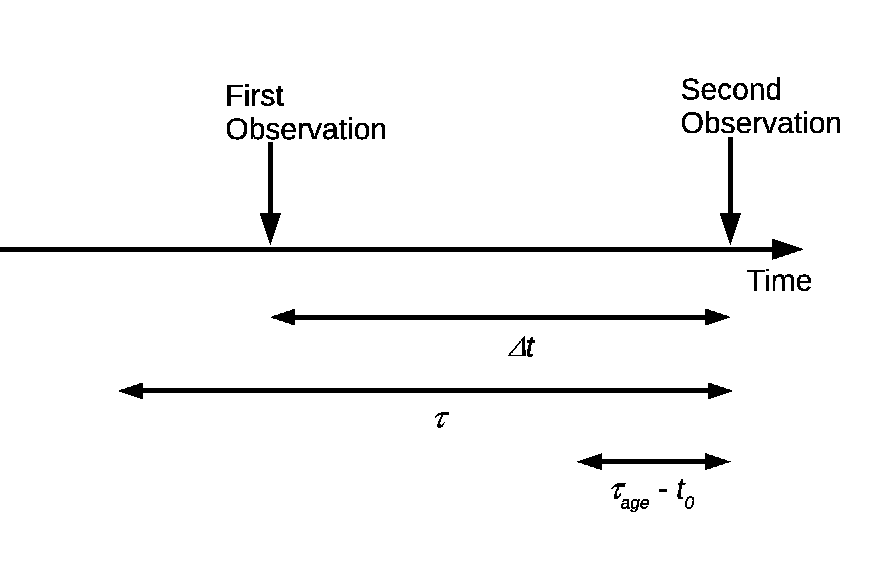
Let us now assume that the event can only be detected a time $t_{0}$ after its occurrence, that it remains visible for a time $\tau$ and that we are only interested in events younger than $\tau_{\rm age}$ (see Figure 1).

Refer to caption — Figure 1: The different variables used in this calculation. $t_{0}$ is defined as the time when the luminosity is above a certain threshold value which makes the object detectable, $\tau$ is defined as the time period where the transient can be detected and $\tau_{\rm age}$ is an arbitrary age since explosion, with $\tau_{\rm age}-t_{0}$ being the time period where events younger than $\tau_{\rm age}$ can be detected.

The event will be detectable younger than $\tau_{\rm age}$ only if $\tau_{\rm age}\geq t_{0}$ . If this is the case, the time period where events not seen in the first observation could occur and be detected in the second observation will now be the minimum between $\Delta t$ , $\tau_{\rm age}-t_{0}$ and $\tau$ (see Figure 2).

Thus, the probability of no events occurring in this time interval and no detections being made, $P_{\rm ND}^{\rm age}$ , will be:

\displaystyle P_{\rm ND}^{\rm age}=\exp\biggl[-R~\min\{\Delta t,\ \max(\tau_{\rm age}-t_{0},\ 0),\ \tau\}\biggr].

(4)

With this information, the probability of detecting one or more events in the second observation will be simply $1-P_{\rm ND}^{\rm age}$ .

Cadence choice

Using the formula above, we could try maximizing the probability of detection. For a fixed target, this can only be done decreasing the cadence, $\Delta t$ , as long as the number of targets that are observed in the sample is not compromised significantly.

It is easy to see that, if $\tau_{\rm age}>t_{0}$ , increasing $\Delta t$ from zero to larger values will increase the probability of detection only while $\Delta t<\min(\tau_{\rm age}-t_{0},\tau)$ . For bigger cadences the probability will stay constant. Thus, a natural choice for the cadence would be $\Delta t=\min(\tau_{\rm age}-t_{0},\tau)$ .

If larger cadences were chosen, the probability of detecting events younger than $\tau_{\rm age}$ would not change, but not all detected events would be guaranteed to be younger than $\tau_{\rm age}$ , which could be a problem if a fast age estimation is required. On the other hand, larger cadences would increase the probability of detecting older events, up to when $\Delta t>\tau$ , when the probability of detecting an event of any age would remain constant too.

Choosing $\Delta t=\min(\tau_{\rm age}-t_{0},~\tau)$ has the added benefit that if $\tau_{\rm age}$ is smaller than the rise time and the object type was known, the absolute magnitude of the event could be used as an age estimator. This is because the event would be guaranteed to be rising at detection time and the magnitude–age relation would be single–valued. In reality, there could be events of different types simultaneously occurring which would make the age determination only useful in a statistical sense.

In general, $\Delta t$ will be a function of the distance and light curve of the variable object to be detected, but also of the desired age of detection, $\tau_{\rm age}$ . Hence, for young and bright objects with extended light curves, the cadence should be set to at least $\tau_{\rm age}-t_{0}$ if we want to increase the cadence while maximizing the detection of events with a given age.

However, it is not always easy to repeat the observations with a fixed cadence. Bad weather, the change of position of the targets throughout the year or the appearance of other objects of interest, among many reasons, may cause the cadence between observations to vary.

An alternative strategy is to let the cadence adapt individually in a sequence of observations in order to maximize the detection probabilities.

Detection probabilities for a sequence of observations

Now, we compute the probability of not detecting any new events in a sequence of observations, $P_{\rm ND,~Total}^{\rm age}$ .

We note that for no events to be detected, each individual observation must result in negative detections, i.e. we have:

	$\displaystyle P_{\rm ND,~Total}^{\rm age}$	$\displaystyle=\Pi_{i}~\exp\Bigl[-R^{i}~\min\{\Delta t^{i},\ \max(\tau_{\rm age}-t_{0}^{i},\ 0),\ \tau^{i}\}\Bigr]$
		$\displaystyle=\exp\Bigl[-\Sigma_{i}~R^{i}~\min\{\Delta t^{i},\ \max(\tau_{\rm age}-t_{0}^{i},\ 0),\ \tau^{i}\}\Bigr],$		(5)

where the indices indicate different targets. Thus, the probability of detecting one or more new events will be:

\displaystyle P_{\rm D,~Total}^{\rm age}

\displaystyle=1-\exp\Bigl[-\Sigma_{i}~R^{i}~\min\{\Delta t^{i},\ \max(\tau_{\rm age}-t_{0}^{i},\ 0),\ \tau^{i}\}\Bigr].

(6)

With this formula, we recover the expected number of events in the entire observational sequence, which is the term inside the exponential, i.e. in $P_{\rm D,~Total}^{\rm age}=1-\exp(-\lambda_{\rm D,~Total}^{\rm age})$ ,

\displaystyle\lambda_{\rm D,~Total}^{\rm age}=\Sigma_{i}~R^{i}~\min\{\Delta t^{i},\ \max(\tau_{\rm age}-t_{0}^{i},\ 0),\ \tau^{i}\}

(7)

is the expected number of new detected events with the required age. Thus, we can use either equation (6) or (7) to determine the fitness of individual schedules, but we recommend using equation (7).

Limited number of targets

It is possible that the number of targets available for detecting new events with a given age is too small, i.e. assuming a fixed exposure time and cadence for all observations, that the number of visible targets where $\tau_{\rm age}>t_{0}$ is smaller than the length of the night divided by the exposure time.

For very short–lived transient surveys this is not a problem, since even with relatively small cadences $\Delta t>\tau$ , and the probability of detection in an individual observation would be $p\approx R~\tau$ , i.e. it would be almost independent of the cadence or how many times we observe a target per night.

In relatively long–lived transient surveys, i.e. time–scales of days or longer, we would not want to repeat targets in a given night. This is because when $\Delta t<t_{\rm age}-t_{0}$ the probability of detection in an individual observation is $P\approx R~\Delta t$ . Thus, many observations to a given target in a given night would be almost equivalent to observing the target once per day or once every few days in terms of probabilities, but with a significantly higher cost on the resources and preventing the telescope from observing other targets.

In general, the number of targets for a given cadence should be of the order of the fraction of time that we want to spend in that sample per night, $f$ , times the total number of observations per night, $N_{\rm exp}$ , times the cadence, $\Delta t$ . The detection rate would be approximately the multiplication of this number with the typical rate of occurrence, $R$ .

Hence, a possible strategy would be to order targets by the time that it takes for the events of interest to be detectable, $t_{0}$ , depending on their distance and extinction, select a detection age according to scientific criteria, and then group the targets according to the resulting cadence and sample sizes. This is summarized in the following table:

Table 1: For a desired detection age (

\tau_{\rm age}

) we show a possible choice of cadence in days (

\Delta t

), the maximum sample size consistent with this cadence and the approximate detection rate if the suggested cadence and maximum sample sizes were used.

t_{0}

corresponds to the time for the transient events to become visible since its occurrence,

N_{\rm exp}

is the number of observations per night and

R

is the rate of events expected in each field. We assume that in all cases the time that a transient remains visible,

\tau

, is bigger than the cadence chosen. For the opposite case,

\Delta t

can be replaced by

\tau

in the last two columns below:

Age	Reference Cadence	Sample size	Approx. detection rate
$\tau_{\rm age}$	$\Delta t=\langle\tau_{\rm age}-t_{0}\rangle$	$f~N_{\rm exp}~\Delta t$	$f~N_{\rm exp}~\Delta t~\langle R\rangle$

2.1 Genetic algorithm

As discussed above, one can let the cadence vary from observation to observation and from object to object. For an ideal schedule, we would like to select the optimal combination of cadences that can adapt to unexpected changes of the observational plan. For this, we use the probability of detection, or the expected number of events, of a sequence of observations as the fitness indicator and we use a genetic algorithm to find the best available observational plan for the following night. This can reflect unexpected changes to the observational plan in a daily basis, and can be extended to fractions of a night optimizations if necessary.

We have used the genetic algorithm implemented in RTS2 [5], taking into account the cadence to each target ( $\Delta t$ ) and the distance, event rate, height above the horizon and sky brightness, all of these reflected in the quantities $t_{0}$ and $\tau$ , to build the observational plan.

The distance between targets is also taken into account indirectly. If it is too big, the number of visited targets per night, or the number of terms in Equation (7), will be reduced and the probability of detection will decrease accordingly. Similarly, when the targets are too distant, or too close to the horizon, or the sky too bright, $t_{0}$ will increase and $\tau$ will decrease, decreasing the detection probabilities too. The bigger the event rate in every target, the bigger the detection probability, which will favour those targets with the biggest intrinsic rates. Finally, the time since last observation will determine the cadence, changing the detection probabilities as well.

In these calculations, the time between targets is computed using the maximum between the slew time and the readout time, which effectively defines a disk around each target where the time penalty is constant. Reaching the outer circumference of this disk would take exactly the readout time assuming that the CCD can read out electrons while simultaneously slewing in the most efficient trajectory. This is regularly accomplished by RTS2, since it optimizes observations by reading out electrons and moving to a new position simultaneously.

For instance, a readout speed of about 2 sec and a slew speed of 5 deg sec^-1 define a disk around the previous target of about 10 deg in the sky where the time penalty for new targets is the same. In most telescopes the slewing movement is accomplished with two independent motors, which makes the size and shape of this disk really depend on the initial configuration of the telescope before slewing, and whether an equatorial or altazimuthal mount is used.

The details of the genetic optimizer, based on the NSGAII algorithm [7], are described in detail in [8]. It is worth mentioning that the genetic algorithm can handle multiple objectives, which can be used to find the Pareto front of optimal values instead of a single solution, e.g. look for multiple detection ages, which we have also implemented (see Figure 4).

The Pareto front is the locus of solutions in a multi–objective optimization problem where one objective cannot be improved without compromising the other objective functions. For example, in an optimization problem with two objective functions, for every value of one of the two objective functions there is an optimal value for the remaining objective function, i.e. the Pareto front can be composed by infinite solutions.

2.2 Calculation of $t_{0}$ and $\tau$

In the previous sections we did not include the calculation of the time for an event to become detectable, $t_{0}$ , and the time that an event remains detectable, $\tau$ . These terms can be computed from empirical light curves of the particular event to be detected, and can be stored as functions of the critical luminosity above which the object can be detected.

Thus, the problem is reduced to computing the flux above which the object can be detected. To do this, we solve the signal to noise equation for an arbitrary value above which we define an object to be detected, e.g. $S/N=5$ . This equation is:

\displaystyle S/N(t)=\frac{\gamma_{\rm TE}^{\rm CCD}(t)~T}{\bigl[\gamma_{\rm TE}^{\rm CCD}(t)~T+\gamma_{\rm sky}^{\rm CCD}~T~n_{\rm pix}+\gamma_{\rm RN}^{2}~n_{\rm pix}\bigr]^{1/2}},

(8)

where $S/N(t)$ is the signal to noise ratio as a function of time, $\gamma_{\rm TE}^{\rm CCD}(t)$ are the photons per unit time detected by the CCD from the transient event as a function of time, $T$ is the exposure time, $\gamma_{\rm sky}^{\rm CCD}$ are the photons per unit time coming from the sky and detected in one pixel of the CCD, $n_{\rm pix}$ is the number of pixels used to do photometry and $\gamma_{\rm RN}$ is the readout noise per pixel of the CCD. In general, $n_{\rm pix}$ is a function of the seeing at the zenith and the angle from the zenith.

Solving the previous quadratic equation for $\gamma_{\rm TE}^{\rm CCD}(t)$ with a given value of $S/N$ and choosing the positive root gives the following result:

\displaystyle\gamma_{\rm TE}^{\rm CCD}(t)=\frac{S/N^{2}}{2~T}~\Biggl[1+\biggl(1+\frac{4~n_{\rm pix}}{S/N^{2}}\{\gamma_{\rm RN}^{2}+\gamma_{\rm sky}^{\rm CCD}~T\}\biggr)^{1/2}\Biggr].

(9)

Now, we can include the effect of distance, collecting area, spectral shape and CCD characteristics in the following equation:

\displaystyle\gamma_{\rm TE}^{\rm CCD}(t)=\frac{A}{4\pi D^{2}}~\int\gamma_{\rm TE}^{\nu}(t)~\eta_{\nu}~d\nu

(10)

where $A$ is the collecting area of the telescope, $D$ is the distance to the object, $\gamma_{\rm TE}^{\nu}(t)$ is the number of photons per unit time per unit solid angle per unit frequency of the transient event as a function of time since occurrence, $\eta_{\nu}$ is the efficiency with which the photons are captured as a function of frequency, which depends on the reflecting surfaces, intervening lenses, CCD quantum efficiency and filters.

We can write a similar equation for the photons coming from the sky in every pixel of the CCD:

\displaystyle\gamma_{\rm SKY}^{\rm CCD}(t)=\frac{\Delta\Omega~A}{\cos z}~\int\gamma_{\rm SKY}^{\nu}(t)~\eta_{\nu}~d\nu,

(11)

where $\Delta\Omega$ is the solid angle of one pixel of the CCD, $z$ is the angle from the zenith and $\gamma_{\rm SKY}^{\nu}$ is now the number of photons coming from the sky per unit time per unit area per unit solid angle per unit frequency.

Thus, if we compute $\gamma_{{\rm TE}}^{\rm CCD}(t)$ , assuming the object is at a distance $D$ from the observer, $\gamma_{{\rm TE},D}^{\rm CCD}(t)$ , and $\gamma_{\rm SKY}^{\rm CCD}$ assuming the object is at a given angle $z$ from the zenith, $\gamma_{\rm SKY}^{\rm CCD}(z)$ , for a given sky brightness and for a particular telescope configuration, we can simply scale the results as follows:

	$\displaystyle\gamma_{{\rm TE},D}^{\rm CCD}(t)=\gamma_{{\rm TE},D_{0}}^{\rm CCD}(t)~\biggl(\frac{D_{0}}{D}\biggr)^{2}$		(12)
	$\displaystyle\gamma_{\rm SKY}^{\rm CCD}(z)=\frac{\gamma_{\rm SKY}^{\rm CCD}(0)}{\cos z},$		(13)

Thus, we can now compute the times when the object becomes detectable and when it is no longer detectable, $t_{0}$ and $t_{0}+\tau$ :

	$\displaystyle t_{0},$	$\displaystyle\ t_{0}+\tau=$
		$\displaystyle\biggl(\gamma_{{\rm TE},D_{0}}^{{\rm CCD}}\biggr)^{-1}\Biggl\{\biggl(\frac{D}{D_{0}}\biggr)^{2}\frac{S/N^{2}}{2~T}~\Biggl[1+\biggl(1+\frac{4~n_{\rm pix}}{S/N^{2}}\{\gamma_{\rm RN}^{2}+\frac{\gamma_{\rm sky}^{\rm CCD}(0)}{\cos z}~T\}\biggr)^{1/2}\Biggr]\Biggr\},$		(14)

where $\biggl(\gamma_{{\rm TE},D_{0}}^{{\rm CCD}}\biggr)^{-1}$ is the inverse of the function computed in equation (12), which should have two solutions for a transient which is composed by an early monotonically increasing component followed by a monotonically decreasing late component. Importantly, the inversion of $\gamma_{{\rm TE},D_{0}}^{{\rm CCD}}$ must be performed only once, and can be stored numerically in a table, e.g. in logarithmic intervals of photons per unit time.

Thus, for a given signal to noise ratio ( $S/N$ ), which we arbitrarily define as the value that gives a detection, a given distance from the source ( $D$ ), exposure time ( $T$ ), sky brightness (c.f. $\gamma_{\rm SKY}^{\rm CCD}$ ), seeing (c.f. $n_{\rm npix}$ ), readout noise per pixel ( $\gamma_{\rm RN}$ ) and angle from the zenith ( $z$ ), we can compute $t_{0}$ and $\tau$ , which are necessary for the calculation of the expected number of events and the probabilities of detection in an individual target and a sequence of observations.

It is important to note that the detection of objects is sometimes performed using individual pixels, in which case we can set $n_{\rm pix}$ to one, and multiply the term $\gamma_{\rm TE}^{\rm CCD}(t)$ in equation (8) by the fraction of photons that fall in the central pixel in the position of the object, depending on the seeing conditions, which would result in the following modified equation:

	$\displaystyle t_{0},$	$\displaystyle\ t_{0}+\tau=$
		$\displaystyle\biggl(\gamma_{{\rm TE},D_{0}}^{{\rm CCD}}\biggr)^{-1}\Biggl\{\biggl(\frac{D}{D_{0}}\biggr)^{2}\frac{S/N^{2}}{2~f~T}~\Biggl[1+\biggl(1+\frac{4}{S/N^{2}}\{\gamma_{\rm RN}^{2}+\frac{\gamma_{\rm sky}^{\rm CCD}(0)}{\cos z}~T\}\biggr)^{1/2}\Biggr]\Biggr\},$		(15)

where $f$ is the fraction of the light from a point source that would fall in one pixel in the position of the object, generally a function of the seeing at the vertical, the angle from the zenith and the frequency of the photons to be detected.

3 Results and discussion

In Figures 3 and 4 we present example implementations of the scheduling strategy presented in this work with the genetic algorithm used in RTS2.

Figure 3 shows the probability of finding supernova with a reference 50 cm telescope in an observational plan composed of 60 sec individual exposures, with simulated cadences and supernova rates in each field. We can see the probability increasing with each generation of observational plans and then staying constant. Each generation is formed by a population of 1,000 different observational plans and the initial iteration consisted of a series of randomly generated targets for each observational plan of the population, which were crossed and mutated to obtain the best observational plans.

Figure 4 shows the space of optimal solutions when two objective functions are used. This is, the Pareto front of non–dominated solutions, or the space of solutions where one variable is at its optimal value without compromising the other variables. In this simulation we use the objective functions: (1) probability of finding supernovae before maximum and (2) the probability of finding supernova younger than three days from explosion, using similar parameters to those used in the simulation shown in Figure 3.

Interestingly, we have used the already implemented genetic scheduler from RTS2 to find the schedule that maximizes the average height above the horizon for our list of targets, or that minimizes the typical distance between targets. For both cases, we have found that the probability of detection of the resulting schedule is smaller by more than a factor of two with respect to our method, which suggests that our strategy is significantly better for finding transient objects.

Thus, the implemented scheduling strategy based on maximizing the probability of finding new transient events is able to obtain significantly higher detection probabilities than alternative methods. We were able to build observational plans for every night to maximize the probability of detecting particular events, or similarly, the expected number of detections. These plans were based on pre–defined samples of targets that have characteristic cadence and exposure times, and that can easily adapt to unforeseen changes in the scheduled observations.

In order to compute the observational plans with the highest detection probabilities, we used the genetic algorithm implemented in the telescope control system RTS2, where a multi–objective algorithm selects the optimal sequence of observations for our purposes.

We expect to be able to extend this work to scheduling of coordinated networks of robotic telescopes looking for specific types of transient events, or looking for many different phenomena if multi–objective optimization is used. We also expect to release the implementation in a future version of RTS2 (http://rts2.org).

An important question is whether this method is able to recompute the optimal observational plan when unexpected changes in the sequence of observations occur. In a single computer, with the current implementation of the code we cannot think of simple ways of achieving this, since it normally takes many hours to find the optimal observational plan or set of Pareto–optimal plans in a single PC. However, with faster computers, pre–calculating detection probabilities for every target at every time in the night, and given that genetic algorithms can be relatively easily parallelised, we expect this to be feasible in the near–future.

Alternatively, one could switch from using optimized observational plans to computing the detection probabilities for every available target and choose the one with the highest detection probability every time the telescope has finished integrating, taking into account the slew and readout time by subtracting the expected cost of slewing in term of detection probabilities per unit time for the corresponding slewing times.

Finally, it should be noted that this method is not exclusive for supernova transients, but to any transient with well characterized light–curves and with well understood target fields.

4 Application to the new 50 cm robotic telescope for CHASE

The CHASE survey [6] is the most prolific nearby supernova search in the southern hemisphere. It finds more than 70% of the nearby ( $z<0.3$ ) supernova in the southern hemisphere, with discovery ages much younger than competing surveys (see Figure 5). CHASE uses a fraction of the time available in four of the six PROMPT telescopes [1] located in CTIO.

In order to expand the capabilities of CHASE and to have a better control over the scheduling of the observations, we are in the process of purchasing and installing a 50 cm robotic telescope that will join the other PROMPT telescopes for the SN survey and follow up.

The telescope will be a 50 cm automated telescope: composed of an optical tube, a CCD camera with a set of filters, a mount, a meteorological station, a dome and computers for controlling and analyzing the data. It will be located in CTIO and remotely controlled from Cerro Calán (Santiago, Chile). It will observe hundreds of targets every night with the aim of doubling the observing capabilities of the CHASE survey and to try new observing strategies with new associated scientific goals.

The optical tube of the telescope will be a 50 cm aperture Ritchey–Chretien design, with a focal ratio of 12, in an open–truss carbon fiber tube purchased from the Italian company Astrotech. The camera will be a 2kx2k pixels Finger Lakes Proline camera, with a back illuminated, UV enhanced, 95% peak quantum efficiency Fairchild 3041 CCD. The pixel size will be 0.52^′′ and the field–of–view will be 17.6^′ in side. The camera will be equipped with a 12–slot filter wheel with the filters u’g’r’i’, Johnson B and V and WFCAM Z, purchased from Asahi–Spectra (see transmission curves in Figure 6).

The camera was chosen to avoid the potential presence of residual images in the imaging of targets, which currently dominate our SN candidate lists with the PROMPT telescopes, to obtain a relatively big field–of–view, which would allow us to image enough reference stars to do an accurate image alignment and subtraction, but also to obtain the best available quantum efficiency, which is a cost–effective way of collecting more photons per target.

The mount will be the Astro–Physics 3600GTO “El Capitán” model, which is a German equatorial mount with sub-arcmin pointing errors, and a slew speed of about 5 $\deg\ \sec^{-1}$ . The dome of the telescope will be built in Chile and is currently in the design phase.

The scheduling of the observations will be done with the strategy presented in this work, and we expect to start collaborations with other groups using this scheduler in an integrated fashion. For more information please contact the authors.

Acknowledgment. We acknowledge an anonymous referee whose help and guidance lead to significant improvements to the manuscript. F.F. acknowledges partial support from GEMINI-CONICYT FUND. G.P. acknowledges partial support from the Millennium Center for Supernova Science through grant P06-045-F funded by “Programa Bicentenario de Ciencia y Tecnología de CONICYT” and “Programa Iniciativa Científica Milenio de MIDEPLAN”.

References

[1] D. Reichart et al. “PROMPT: Panchromatic Robotic Optical Monitoring and Polarimetry Telescopes”, astro-ph/0502429, 2005.
[2] S. C. Keller et al., ”The SkyMapper Telescope and The Southern Sky Survey”, Publications of the Astronomical Society of Australia 24 (1): 1–12, 2007
[3] T.M. Brown et al., “Las Cumbres Observatory Global Telescope”, American Astronomical Society Meeting Abstracts, 214, 409.14, 2009.
[4] Z. Ivezić et al., “LSST: From science drivers to reference design and data products”, astro–ph/0805.2366.
[5] P. Kubánek et al., “RTS2 – Remote Telescope System, 2nd version”, Gamma Ray Bursts: 30 years of discovery: Gamma Ray Burst Symposium. AIP Conference Proceedings, Vol 727, 2004.
[6] G. Pignata et al., “The CHilean Automatic Supernova sEarch (CHASE)”, Probing stellar populations out to the distance Universe: Cefalu 2008, AIP Conference Proceedings, Vol 1111, 2009.
[7] Deb, K., Pratap. A, Agarwal, S., and Meyarivan, T., “A fast and elitist multi-objective genetic algorithm: NSGA-II”. IEEE Transaction on Evolutionary Computation, 6(2), 181-197, 2002.
[8] P. Kubánek, “Genetic algorithm for robotic telescope scheduling”, Master’s thesis, Universidad de Granada, 2007.

*