On the evolution of environmental and mass properties of strong lens galaxies in COSMOS Thanks: Based on observations made with ESO telescopes at Paranal observatory under program ID 077.A-0473(A) and under large program ID 175.A-083911.
Abstract
Context. Nearly 100 new strong lens candidates have been discovered in the COSMOS field. Among these, 20 lens candidates with 0.341.13, feature multiple images of background sources.
Aims. Using the multi-wavelength coverage of the field and its spectroscopic follow-up, we characterize the evolution with redshift of the environment and of the dark-matter (DM) fraction of the lens galaxies.
Methods. We present spectroscopic and new photometric redshifts of the strong lens candidates. The lens environment is characterized in the following way: we account for the projected 10 closest galaxies around each lens and for galaxies with a projected distance less than 1 Mpc at the lens galaxy redshift. In both cases, we perform similar measurements on a control sample of "twin" non-lens early type galaxies (ETGs). In addition, we identify group members and field galaxies in the X-ray and optical catalogs of galaxy groups and clusters. From those catalogs, we measure the external shear contribution of the groups/clusters surrounding the lens galaxies. The systems are then modeled using a SIE for the lens galaxies plus the external shear due to the groups/clusters.
Results. We observe that the average stellar mass of lens galaxies increases with redshift. In addition, we measure that the environment of lens galaxies is compatible with that of the twins over the whole redshift range tested here. During the lens modeling, we notice that, when let free, the external shear points in a direction which is the mean direction of the external shear due to groups/clusters and of the closest galaxy to the lens. We also notice that the DM fraction of the lens galaxies measured within the Einstein radius significantly decreases as the redshift increases.
Conclusions. Given these, we conclude that, while the environment of lens galaxies is compatible with that of non-lens ETGS over a wide range of redshifts, their mass properties evolves significantly with redshift: it is still not clear whether this advocates in favor of a stronger lensing bias toward massive objects at high redshift or is simply representative of the high proportion of massive and high stellar density galaxies at high redshift.
Key Words.
Cosmology: Gravitational lensing1 Introduction
In the field of gravitational lensing, studies of strong galaxy-galaxy lenses have recently become possible on statistical grounds. Indeed, within just a few years, searches in the SDSS (SLACS: Bolton et al. 2006, 2008, Allam et al. 2007), in COSMOS (Faure et al. 2008, hereafter Paper I; Jackson 2008) and in the CFHT-LS surveys (SL2S: Cabanac et al. 2007, Limousin et al. 2009b) have delivered more than two hundred new strong galaxy-galaxy lenses, spanning a wide range in redshift and image angular separation. The reasons for this interest are several. First, strong lens galaxies provide measurements of the total mass distribution on galaxy scales, bringing additional information about the processes of galaxy formation and evolution (e.g. Ofek et al. 2003, Chae et al. 2006, Koopmans et al. 2006, Tortora et al. 2010). Second, from a statistical point of view, strong lensing occurrences trace the abundance and concentration of matter in the universe, providing another test for cosmological models (e.g. Keeton 2001, Bartelmann et al. 2003).
Studies of the physical and environmental properties of low redshift strong lens galaxies (z0.3) have shown that they are bona-fide massive ETGs (Treu et al. 2006, 2009 -T09 hereafter-, Gavazzi et al. 2007, Grillo et al. 2009). The strong lens sample in the COSMOS field (Paper I), spans a higher redshift range (0.33z1.13) and previous work on this sample have shown that the projected distribution of lens galaxies in COSMOS is comparable to that of ETGs, whether in rich environments such as cosmic filaments, or in the field (Faure et al. 2009, hereafter Paper II). Interestingly, this result means that multiple-mass-sheets do not contribute significantly to make more efficient lenses, contrary to results found in ray tracing through numerical simulations (Wambsganss et al. 2005, Hilbert et al. 2007, 2008). In Paper II we also demonstrate that the presence of large scale structures (LSS) in the lens galaxy environment increases the angular separation of the lensed images of a source, as noticed earlier by Oguri et al. (2005).
In addition, analyses of the mass density profiles of strong lens galaxies from hydrodynamical N-body simulations (Dobke et al. 2007, Limousin et al. 2009a) and lens samples (Limousin et al. 2007, Auger 2008, Natarajan et al. 2009) show that the mass distribution in galaxies depends on their environment. For example, compared to galaxies centrally placed in their group or cluster, some skewing of the total mass density slope appears in galaxies located at the edges of a group or cluster. This is consistent with tidal stripping of their dark matter halo (T09).
Therefore, it is important to explore the local environment of the COSMOS strong lenses rather than LSS as in Paper II. We also want to learn about the lens galaxy mass properties, in particular to derive information relative to their DM fraction (fDM, defined as fDM=1-M⋆/(M⋆+MDM). This is possible as the COSMOS strong lenses pertain to one of the best studied region of the sky, for which deep multi-wavelength observations have been collected (Koekemoer et al. 2007, Taniguchi et al. 2007, Capak et al. 2007a, Scoville et al. 2007, Lilly et al. 2007, Ilbert et al. 2009). Thus the properties of the COSMOS galaxy population have been studied extensively (e.g. McCracken et al. 2007, Capak et al. 2007b, Scarlata et al. 2007a, 2007b, Ilbert et al. 2010).
The paper is organized as follows. In 2, we provide improved redshifts and stellar masses of the COSMOS lens galaxies. In 3, we examine and discuss the lens environment. In 4, we present results from our strong lens mass models for the sub-sample of triple and quadruple image systems. Discussion and conclusions appear in 5. Throughout this paper, we assume a WMAP5 CDM cosmology with , , km s-1 Mpc-1.
2 The COSMOS sample of strong lenses: new redshifts and stellar masses
By visual inspection of stamp images of 10″10″ around 9500 early photometric type galaxies (with redshifts : 0.2 z 1.0, and absolute magnitude: M -20) in the COSMOS field, we have discovered 60 strong lens candidates (Paper I). In addition, in the same study, 7 lens candidates were found serendipitously across the field. Among the whole sample, 19 systems display long curved arcs or multiple images with similar colors (based on SUBARU images, by Taniguchi et al. 2007) around a bright lens galaxy, and with an image arrangement around the lens galaxy which is consistent with the lensing hypothesis, as probed by lens modeling.
Independently, Jackson (2008) inspected the complete set of galaxies in the COSMOS field, without discrimination. He has discovered two additional convincing strong lens candidates producing multiple images: J095930.93+023427.7 and J100140.12+020040.9. The lens galaxies both appear to be ETGs.
Among the 21 multiple image lenses now available, one system (COSMOS 5921+0638) – being the only confirmed lensed quasar of the sample – has been studied separately by Anguita et al. (2009, hereafter Paper III). Another system, COSMOS 5737+3424, is a galaxy cluster that is lensing a set of background galaxies. In such a case, the lens covers a different mass scale than in the other 20 systems, and the lens potential is more complex than a single lens galaxy: this target has been dropped from the present analysis.
2.1 Spectroscopic followup


On March 3rd and April 25-26th 2006, we have successfully obtained spectra for five of the strong lenses in the COSMOS field (PI: Faure) using the FORS1 instrument (ESO/VLT) in multi-object spectroscopic mode with 19 slits. For each target, the central slit was located on the lens candidate with an orientation intersecting both the lens galaxy and the brightest lensed image. The other 18 slits in the 7’x7’ field around the lens, were preferentially positioned on galaxies with colors similar to that of the lens galaxy (likely at the same redshift). Leaving aside COSMOS 5921+0638 (discussed in Paper III) and the lens cluster COSMOS 5737+3424, we display the spectra of the other three lens galaxies in Fig. 1. Regarding the source redshifts, from this dataset we could extract only one source redshift, in COSMOS 5921+0638 (Paper III). Positions and redshifts of secondary targets around COSMOS 0012+2015, COSMOS 0013+2249 and COSMOS 0049+5128 are given in Table 2.
In addition, several COSMOS lens candidates have been observed with the Keck telescopes.
Using the Deep Extragalactic Imaging Multi-Object Spectrograph (DEIMOS) a spectrum of COSMOS 0018+3845 has been obtained on February 11, 2010 (Fig. 2). The data were collected in 71800s exposures under photometric conditions with 0.5-0.7″ seeing. We used a 1″ slit together with the 830 line/mm grating tilted to 7860Å and the OG550 blocking filter. The resulting spectral resolution is Å, depending on seeing and object morphology. The objects were dithered along the slit by ″ between exposures to improve background subtraction, as described in Capak et al. (2009). The redshift of the lens has been identified using the CaII H & K absorption lines and G-band. The source redshift is estimated based on the Lyman break which is somewhere in the Subaru IA624-band (=6226 Å, FWHM=299Å), putting constraints on the source redshift: 3.9z4.1. From there, we find that for =3.960.02, SiIV and CII would align with spectral absorption features of the lens. This estimation of the source redshift is used throughout the paper.
Moreover, with the Low Resolution Imaging Spectrometer (LRIS), Lagattuta et al. (2010) measured the redshifts for seven lens galaxies and two sources.
Finally, from the z-COSMOS catalog (Lilly et al. 2009) we have retrieved the redshifts of seven strong lens candidates from our list (based on the G-band and MgI absorption lines). Two of them, re-observed with Keck/LRIS, benefit from a second redshift determination from a higher signal-to-noise spectrum. Both redshifts are in agreement.
A summary of the spectroscopic observations available for this sample is given in Table 1, while the lenses’ redshifts are provided in Table 3.
| Name | Instr. | E.T. |
| ks | ||
| COSMOS 0012+2015 | FORS1 | 1.8 |
| COSMOS 0013+2249 | FORS1 | 1.2 |
| COSMOS 0049+5128 | FORS1 | 1.2 |
| COSMOS 5921+0638 | FORS1 | 1.8 |
| COSMOS 0050+4901 | VIMOS | 3.6 |
| COSMOS 0056+1226 | VIMOS | 3.6 |
| COSMOS 5947+4752 | VIMOS | 3.6 |
| J095930.93+023427.7 | VIMOS | 3.6 |
| COSMOS 5857+5949 | VIMOS | 3.6 |
| COSMOS 0124+5121 | VIMOS | 3.6 |
| COSMOS 0227+0451 | VIMOS | 3.6 |
| COSMOS 0018+3845 | DEIMOS | 12.6 |
| COSMOS 0038+4123 | LRIS | 3.6 |
| COSMOS 0050+4901 | LRIS | 5.4 |
| COSMOS 0056+1226 | LRIS | 5.4 |
| COSMOS 0211+1139 | LRIS | 5.4 |
| COSMOS 0216+2955 | LRIS | 3.6 |
| COSMOS 0254+1430 | LRIS | 1.2 |
| J100140.12+020040.9 | LRIS | 5.4 |
| RA | DEC | z |
| COSMOS 0012+2015 | ||
| 150.01554 | 2.3105342 | 0.492 |
| 150.05263 | 2.3377222 | 0.378 |
| 150.07391 | 2.3256596 | 0.222 |
| 150.07463 | 2.3485102 | 0.217 |
| 150.07239 | 2.3679651 | 0.344 |
| 150.08564 | 2.3641732 | 0.340 |
| 150.10210 | 2.3524922 | 0.220 |
| 150.11477 | 2.3328146 | 0.373 |
| COSMOS 0013+2249 | ||
| 150.10193 | 2.3900368 | 0.218 |
| 150.09001 | 2.3836205 | 0.530 |
| 150.08210 | 2.3904710 | 0.351 |
| 150.07843 | 2.3895686 | 0.352 |
| 150.07239 | 2.3679506 | 0.347 |
| 150.06510 | 2.3855444 | 0.343 |
| 150.05808 | 2.3804333 | 0.346 |
| 150.05235 | 2.3837337 | 0.350 |
| 150.03149 | 2.3745112 | 0.220 |
| 150.02774 | 2.3738948 | 0.222 |
| 150.00332 | 2.4075260 | 0.347 |
| COSMOS 0049+5128 | ||
| 150.23256 | 1.8862956 | 0.673 |
| 150.23365 | 1.8704970 | 0.283 |
| 150.21829 | 1.8847159 | 0.621 |
| 150.20779 | 1.8823028 | 0.026 |
| 150.20824 | 1.8753444 | 1.146 |
| 150.20526 | 1.8578028 | 0.337 |
| 150.19758 | 1.8606685 | 0.267 |
| 150.18165 | 1.8552841 | 0.168 |
2.2 Improved photometric redshifts

Recently a new set of photometric redshifts for galaxies in the COSMOS field has been derived by Ilbert et al. (2009), using the code Le Phare (S. Arnouts & O. Ilbert22 2 Available at www.oamp.frpeoplearnoutsLE_PHARE.html) and the photometric dataset by Capak et al. (2007a and 2009). Compared to the previous set of COSMOS photometric redshifts by Mobasher et al. (2007), which relied on 8 broad bands, the main improvement is the use 30 bands: the 8 broad bands plus 12 intermediate bands, 2 narrow bands, 7 bands in the near-infrared and 1 band in the ultra-violet. In Fig. 3 we have displayed a comparison between the new photometric redshifts and spectroscopic redshifts for the 17 lens galaxies in our sample for which we have the two measurements. For most lens galaxies, the agreement is good within the 68% confidence level error-bars measured for the photometric redshifts. Thus, these new photometric redshifts for the lenses are reliable estimates of their spectroscopic redshifts. We notice that three systems show a strongly deviant photometric redshift (COSMOS 0254+1430: zphot=0.460.01 and zspec=0.4170.001; J095930.93+023427.7: zphot=1.10 and zspec=0.8920.001; COSMOS 0018+3845: zphot=0.440.01 and zspec=0.97550.0003). In those three cases, the photometry of the lens galaxy obtained from ground-based data is contaminated by the close and bright images of the source, and the photometric redshift determination is consequently biased.
2.3 Stellar masses of the lens galaxies

We have derived a first set of stellar masses using the Bayesian code described in Bundy et al. (2006). In brief, a data couple, made of the observed galaxy spectral energy distribution (SED) and its redshift, is referenced to a grid of models constructed using the Bruzual & Charlot (2003) synthesis code. The grid includes models that vary in age, star formation history, dust content and metallicity. At each grid point, the probability that the observed SED fits the model is calculated: the corresponding stellar mass and the stellar mass to K-band luminosity ratio are stored. By minimizing over all parameters in the grid, the stellar mass probability distribution is obtained. The median of this distribution is taken as the stellar mass estimate, while the width corresponding to 68% of the probability distribution encodes the error bar resulting from degeneracies and uncertainties in the model parameter space. The final error bar on the stellar mass also includes the K-band photometric uncertainty as well as the expected error on the luminosity distance that results from the uncertainty on the photometric redshift. The stellar masses and uncertainties are provided in Table 3 and plotted in Fig. 4.
From the ACS-F814W images (Koekemoer et al. 2007) we infer the contamination due to the light coming from the background lensed images in the stellar mass measurements. In an aperture of 3″ radius, the lensed images are 3 to 7 magnitudes fainter than their respective lensing galaxy: in all cases this contamination generates an error on the stellar mass 0.01 dex.
In order to appreciate the reliability of our estimates of the stellar mass (and uncertainties), we have retrieved among the 3.6 IRAC catalog of the Spitzer-COSMOS survey (Sanders et al. 2007) 18 of the 20 strong lenses; the other two lens galaxies were not detected with Spitzer. For these lenses we have compared our estimates of the stellar masses to those inferred by Ilbert et al. (201033 3 The COSMOS catalogs can be found at http://irsa.ipac.caltech.edu/data/cosmos): they are in reasonable agreement (see Fig. 4). The typical difference between the two mass estimators (0.2 dex) is widely discussed in Ilbert et al. (2010). Both distributions show a tendency of increasing lens stellar mass with redshift. This feature will be discussed in more detail in the discussion ( 5.1).
| Name | z | R10 | N1 | M⋆ | Ntwin | |||
|---|---|---|---|---|---|---|---|---|
| lens/source | kpc | log10() M⊙ | ||||||
| COSMOS 0049+5128 | 0.3370.001 | 20.320.01 | 1.31.9 | 1013 | 1.00.9 | 10 | 10.720.08 | 63 |
| COSMOS 5947+4752 | 0.3450.001 | 20.360.01 | 1.91.5 | 947 | 1.60.7 | 13 | 10.650.22 | 59 |
| COSMOS 0013+2249 | 0.3460.001 | 19.630.01 | 6.20.2 | 602 | 2.30.5 | 16 | 11.290.10 | 23 |
| COSMOS 0056+1226 | 0.3610.001/0.8080.001 | 19.770.01 | 1.41.2 | 996 | 1.10.7 | 11 | 11.260.13 | 42 |
| COSMOS 5857+5949 | 0.3720.001 | 20.550.01 | 0.94.5 | 1348 | 0.42.2 | 5 | 10.810.09 | 69 |
| COSMOS 0012+2015 | 0.3780.001 | 19.950.01 | 1.91.1 | 833 | 1.10.7 | 12 | 11.140.09 | 40 |
| COSMOS 0254+1430 | 0.4170.001/0.7790.001 | 19.760.01 | 0.53.5 | 1767 | 0.61.1 | 5 | 11.530.17 | 28 |
| COSMOS 5921+0638 | 0.5510.001/3.140.05 | 20.820.01 | 0.64.1 | 1939 | 0.41.6 | 3 | 10.790.10 | 51 |
| COSMOS 0216+2955 | 0.6080.001 | 20.710.01 | 4.60.3 | 665 | 2.70.3 | 19 | 11.380.07 | 29 |
| COSMOS 0038+4133 | 0.7380.001 | 21.030.01 | 5.50.9 | 585 | 1.90.5 | 17 | 11.620.03 | 30 |
| COSMOS 0124+5121 | 0.8560.001 | 22.610.02 | 2.91.0 | 777 | 2.10.4 | 15 | 10.780.08 | 140 |
| COSMOS 0047+5023 | 0.870.01 | 21.350.01 | 2.34.8 | 851 | 1.30.7 | 11 | 11.700.04 | 22 |
| J100140.12+020040.9 | 0.8790.001 | 22.010.01 | 0.64.7 | 1931 | 0.32.6 | 2 | 11.160.04 | 94 |
| COSMOS 5941+3628 | 0.880.01 | 21.600.01 | 2.50.4 | 946 | 2.00.3 | 12 | 11.540.06 | 39 |
| J095930.93+023427.7 | 0.8920.001 | 21.980.01 | 1.22.4 | 1131 | 0.80.9 | 7 | 11.020.05 | 92 |
| COSMOS 0211+1139 | 0.920.01 | 21.650.01 | 1.80.6 | 948 | 1.60.4 | 13 | 11.760.04 | 31 |
| COSMOS 0050+4901 | 0.9600.001 | 22.010.01 | 0.84.9 | 1735 | 0.61.5 | 4 | 11.640.03 | 43 |
| COSMOS 0227+0451 | 0.9750.001 | 22.090.01 | 0.56.8 | 2149 | 1.00.9 | 7 | 11.390.04 | 58 |
| COSMOS 0018+3845 | 0.97550.0003/3.960.02 | 23.430.03 | 1.01.3 | 1799 | 0.3 | 5 | 10.730.06 | 119 |
| COSMOS 5914+1219 | 1.130.10 | 23.000.02 | 0.90.3 | 1832 | 0.71.2 | 3 | 11.390.05 | 45 |
3 The environment of the lens galaxies
Having now more accurate redshift measurements for the lens galaxies and the galaxies in the COSMOS field, we can undertake a study of the local environments of lens galaxies. Indeed, to understand whether high redshift lensing galaxies (z0.3) are representative of the ETG population at their redshift, as the low redshift lens galaxies are (T09, Auger 2008), we study their environment in comparison to the environment of a population of non-lensing ETGs. Our first analysis of the lens environment with regard to LSS (Paper II) led to the conclusion that lens galaxies are indeed evolving in the same environment than their parent population. Lets now zoom into a more local environment for the lens, using neighbor density measurements as defined and used by T09 for the SLACS sample.
3.1 Projected number of neighbors


3.1.1 The neighbor number densities
In T09, the first estimator is the projected number density of galaxies, , inside a circle with radius R10, equal to the projected distance to the ninth closest neighbor of the lens. The neighbor galaxies are defined such as their magnitude is : +3, and the upper or lower bound, z, of their photometric redshift is : where is a function of the lens magnitude and redshift, and lies between 0.012 and 0.020 for our sample (see Ilbert et al. 2009). For the two lenses with incorrect photometric redshifts, we have used their spectroscopic redshift instead and for the search of neighbors, the values associated with their spectroscopic redshift in the photometric catalog; this ensures that we are using the same search box for lens with spectroscopic and photometric redshifts.
The search for neighbors is performed in the photometric redshift catalog of Ilbert et al. (2009) which contains about 1 million objects. The limiting magnitude chosen for the neighbors ensures that the scaling in brightness (thus in mass) between a lens galaxy and its neighbors is the same for all lenses, independently of its magnitude. For the faintest lens in our sample, this upper limit corresponds to the completeness limit of the COSMOS photometric catalog (depth: i 26.2, Capak et al. 2007a). The range chosen for the redshift ensures that, given the error bars on the neighbor photometric redshifts, they are indeed at the same redshift as the lens galaxies (in the 68% confidence limit error bars).
As in T09, we also computed the projected number of galaxies, , inside a circle with radius 1 Mpc, at the lens redshift. To select the neighbors, we have used the same limiting magnitudes and redshift ranges as for the first estimator.
In order to get comparative measurements for a population of galaxies which are not identified as lenses but have the same morphology (early photometric type), similar brightness and redshift properties, we define a control sample of “twins” for each lens galaxy. Those twins have the upper or lower bounds, ztwin, of their photometric redshift such as: with =0.05, and the upper or lower bounds, , of their magnitude such as : I, with =0.05 mag. The dispersion authorized around the value of the lens redshift and lens magnitude ensures that the sample of twins is large enough for the results to be statistically reliable (between 22 and 140 twins, see Table 3). In addition, the range in redshift is small enough to avoid possible biases due to galaxy evolution and the range in magnitude ensures that the flux difference between a lens and its twins remains lower than 5%. We then measure the average number density of neighbors and the average projected number of galaxies in a circle with radius 1 Mpc: for the control “twin” sample.
We notice that, for an obvious lack of spectroscopic information, the twins cannot be selected according to their velocity dispersion as it is the case in the analysis by T09. Yet our match in magnitude and redshift mimics, up to a certain level of accuracy, a match in mass between the lens galaxies and their twins.
3.1.2 Error measurements on the neighbor number densities
In building the photometric catalog of galaxies, masks were necessary to hide bright objects disturbing the galaxy extraction procedure (see Capak et al. 2007a). From these masks we have measured, at each lens and twin location, the surface that was hidden for the extraction. The hidden surface is typically of a few percents of the total surface used to determine or . It only gives a positive contribution to the total error budget on the neighbor density estimates: indeed, the surface covered by the circle of radius R10 would be smaller if the ninth closest galaxy was behind the mask, and if one or more galaxies are hidden behind the mask, the number of galaxies in a circle of radius would be larger. Therefore, for a fixed number of galaxies, the surface has to be smaller. In summary, for a lens galaxy, the total error bar on the neighbor galaxy density is the quadratic sum of the Poisson error and the error due to the use of masks on the surface encompassing the neighbors. For its average twin, the error bar is the quadratic sum of the Poisson error, the error due to the use of masks and the dispersion for the population of twins. The Poisson error largely dominates the error budget for the lens neighbor number densities, while the dispersion largely dominates the error budget for the twins.
3.1.3 Results
The values of , , and depend on the redshift bin and magnitude limit. To circumvent these effects, we only interpret the results in term of ratios: and . These ratios quantify the richness of the environment of the lens galaxies in comparison to the environment of their respective twins. They are provided in Table 3. The average distance encompassing the 9 closest galaxies to the lens is R=1.2 Mpc with a 1 standard deviation of 0.5 Mpc, hence comparable to the radius of 1 Mpc used to calculate . In Fig. 5, we have displayed the ratios and for the COSMOS lenses and for the SLACS lenses (using data from T09), as a function of redshift. A-priori, the two distributions cannot be directly compared as they may have different normalization factors (due to their different lens selection function, source redshift distribution and survey sensitivity). Yet, we notice that in the redshift range common to the SLACS and COSMOS samples (z[0.33,0.50]), the levels of the distributions for and are similar, suggesting that the normalizations are not drastically different. However, in order to avoid any misinterpretation due to intrinsic sample differences, the SLACS sample and the COSMOS sample distributions are analyzed separately.
The number density ratios displayed in Fig. 5 indicate
whether the lens galaxies reside in a typical environment in
comparison to the twin galaxy population. Would this be true, the
number density ratios should be of the order of 1 at every redshift.
This is indeed the
case in average for the lenses in the redshift range studied here.
3.2 X-ray and optically detected galaxy groups and clusters
The validity of the estimators used to characterize the environments of lens galaxies in 3.1 can be checked using the distribution of groups and clusters in the field based on X-ray and spectroscopic data analysis. Indeed, we can access two supplementary pieces of information: (a) the distribution of X-ray emitting gas in the COSMOS field (XMM-Newton survey: Hasinger et al. 2007 and C-COSMOS with Chandra: Elvis et al. 2009), which traces galaxy groups and clusters in the field (Finoguenov et al. 2007 and in prep.), and (b) the identification of optical groups or clusters (Knobel et al. 2009) from the z-COSMOS spectroscopic program (Lilly et al. 2007).
Moreover, as the presence of groups in the direction to the source generates a different lensing potential in comparison to that of a single lens galaxy, it is important, in preparation of the mass modeling in 4 to know: 1) If the lens galaxies are group members. If this is indeed the case, the group has to be modeled as an individual potential in the lens modeling. 2) What contribution in terms of shear is produced by the groups and clusters towards and around the lens galaxy. Most of the time this contribution is simply represented by an ”external shear" whose parameters are optimized while adjusting the lens model. In this paper, we rather intent to measure independently the external shear using the rich dataset that covers the COSMOS field.
| Name | P | N | Cluster | Dist. | |||
|---|---|---|---|---|---|---|---|
| deg | ID (zz, log10(M200), c, r200) | kpc | |||||
| COSMOS 0049+5128 | 0.33 | 13 | 0.0060.001 | 0.0080.003 | -3812 | _ | _ |
| COSMOS 5947+4752 | 0.04 | 3 | 0.0160.003 | 0.0210.005 | 02 | _ | _ |
| COSMOS 0013+2249 | 0.33 | 26 | 0.0230.003 | 0.0250.005 | 810 | #173 (0.3480.005,13.44,4.18,0.55) | 0.5 |
| COSMOS 0056+1226 | 0.76 | 29 | 0.0110.003 | 0.0030.004 | -1830 | #133 (0.3600.005,13.28,4.32,0.48) | 0.3 |
| COSMOS 5857+5949 | 0.58 | 18 | 0.0190.005 | 0.0330.010 | -418 | _ | _ |
| COSMOS 0012+2015 | 0.39 | 31 | 0.0190.002 | 0.0090.006 | -2419 | _ | _ |
| COSMOS 0254+1430 | 0 | 2 | 0.0020.000 | 0.0060.000 | -313 | _ | _ |
| COSMOS 5921+0638 | 0.61 | 24 | 0.0190.004 | 0.0090.012 | -3731 | _ | _ |
| COSMOS 0216+2955 | 0.06 | 5 | 0.0250.003 | 0.0240.004 | 365 | #221 (0.6000.005,13.56,3.82,0.55) | 0.2 |
| COSMOS 0038+4133 | 0.12 | 4 | 0.0040.000 | 0.0140.002 | -44 | _ | _ |
| COSMOS 0124+5121 | 0.20 | 2 | 0.0020.000 | 0.0070.002 | 93 | _ | _ |
| COSMOS 0047+5023 | 0.06 | 4 | 0.0120.002 | 0.0160.003 | -266 | _ | _ |
| J100140.12+020040.9 | 0.20 | 3 | 0.0060.001 | 0.0090.002 | -287 | _ | _ |
| COSMOS 5941+3628 | 0.07 | 7 | 0.0240.003 | 0.0070.004 | 2215 | _ | _ |
| J095930.93+023427.7 | 0.27 | 4 | 0.0060.001 | 0.0160.004 | -451 | #288 (0.6970.006,13.63,3.73,0.56) | 102 |
| COSMOS 0211+1139 | 0 | 3 | 0.0040.000 | 0.0220.005 | 433 | _ | _ |
| COSMOS 0050+4901 | 0.25 | 2 | 0.0010.000 | 0.0060.001 | -164 | _ | _ |
| COSMOS 0227+0451 | 0 | 4 | 0.0020.000 | 0.0050.001 | -196 | # 101 (0.980.01,13.70,3.65,0.53) | 0.5 |
| COSMOS 0018+3845 | 0.38 | 15 | 0.0370.007 | 0.0820.016 | 134 | _ | _ |
| COSMOS 5914+1219 | 0.25 | 17 | 0.0010.000 | 0.0060.001 | -195 | _ | _ |
In the framework of our lensing analysis, each of the group catalogs (X-ray selected versus spectroscopically selected) has certain advantages and disadvantages. The entire COSMOS region has been mapped through 54 overlapping XMM-Newton pointings while additional Chandra observations have mapped the central region (0.9 square degrees). A composite XMM-Newton and Chandra mosaic has been used to detect and measure the fluxes of groups and clusters to a 4 detection limit of erg cm-2 s-1 over 96% of the ACS field. The general data reduction process can be found in Finoguenov et al. (2007, 2009) and the cluster catalog and weak-lensing analysis are presented in Leauthaud et al. (2010). Therefore, the catalog of X-ray selected groups and clusters is homogeneous and covers the entire COSMOS field. However, it is affected by the sensitivity threshold of the X-ray survey, which is different from the sensitivity cut of the optical dataset. Therefore, groups of modest mass could be missing from the X-ray selected catalog, especially around galaxies at high redshift.
Conversely, the catalog of optically selected groups in COSMOS has the advantage of spanning the same brightness range as the optical imaging dataset from which the strong lens candidates and the arcs have been extracted. Even though the faintest galaxies seen on deep images will remain undetected in the shallower spectroscopic z-COSMOS survey, groups can still be traced and assessed from their central brightest galaxies. Then, the parameters of the galaxy groups can be derived by comparing these detections to a catalog of mock-groups subject to the same detection criteria (see Knobel et al. 2009 for an extensive description of the group catalog). The first data release of the z-COSMOS survey (Lilly et al. 2007) covers a fraction of the full COSMOS field, which leaves some of our COSMOS lens candidates outside the coverage of the group catalog.
Let us establish now whether the lens galaxies are group or cluster members ( 3.2.1) and measure the external shear contribution of the groups and clusters at the lens galaxy position ( 3.2.3).
3.2.1 Lens galaxy group members
We cross-correlate the X-ray cluster catalog (Leauthaud et al. 2010) with the sample of strong lenses. We define as a group member, a lens galaxy located within r200 (radius where the matter density is 200 times the critical density) of the group center, and with redshift identical to the group redshift (within error bars). We have found 4 matches and there is a galaxy cluster detected at a lower-redshift in direction to J095930.93+023427.7 (see Table 4).
Using the group catalog built from the optical dataset, we do not identify any new groups associated in redshift and observational plane with lens galaxies than those already identified using the X-ray catalog. In Table 4 we give the probability that galaxies in a 2′2′ field around the lens galaxy are included in the z-COSMOS catalog. This figure establishes roughly the “completeness” of the survey at every lens location and tells us if the z-COSMOS group catalog can be used to characterize the environment of the lens.
3.2.2 Comparison: galaxy group members and projected number density of neighbors
In principle, lens galaxies which are group members are expected to have large neighbor number densities. This should be visible in the ratio measured in 3.1. This is indeed the case with the first estimator for the lens in COSMOS 0013+2249 (=6.20.2) and COSMOS 0216+2955 (=4.60.3), and it is unclear for COSMOS 0056+1226 and COSMOS 0227+0451 because of the large error bar on the measured density ratios. With the second estimator, the ratio are in average lower than with , and it is therefore more difficult to identify correctly an over-dense field. On the contrary, COSMOS 0038+4133 shows a large density ratio (=5.50.9) without being associated to any known galaxy group in X-ray or optic.
3.2.3 The external shear due to clusters and groups
We estimate the shear and convergence produced by the groups (either X-ray or optical) detected around the lens galaxies in order to characterize the contribution of the environment to the total lens potential in future lens models ( 4). To do so we followed the method described in Paper III. In short, we compute the convergence and shear produced by all groups closer in projection than a given radius (5′, as in Paper III), and at any redshift up to that of the source. We assume that the mass profile of every group follows a truncated isothermal sphere (TIS). The choice of this profile is motivated by the fact that the shear and convergence produced by an isothermal sphere are easy to compute (Keeton 2003, Momcheva et al. 2006). Moreover, as we will consider only groups and clusters which do not cross the line-of-sight to the source, estimations of their total masses rather than of their mass distributions are sufficient for the accuracy of the result. We selected a truncated profile to avoid to give unrealistically too much weight to the most distant groups.
The three-dimensional density distribution of the TIS can be written:
| (1) |
where is the truncation radius. The convergence, , and shear, , produced by this profile are respectively:
| (2) |
| (3) |
where is the impact parameter of the TIS, which relates to the Singular Isothermal Sphere (SIS) impact parameter as:
| (4) |
In the limit where these quantities match those of the SIS.
To compute the external shear produced by the groups and clusters we proceed as follows. Whenever P0.3 in Table 4 (column 2), we only consider the catalog of X-ray detected groups and clusters. The groups mass potentials are modeled as TIS using the value M200 and r200 (used as the truncature radius). The error on the X-ray mass comes from the scatter in the relation used to derive the mass from the luminosity (Leautaud et al. 2010): it is of the order of 20% of M200 (Vikhlinin et al. 2009). Whenever P0.3 in Table 4 (column 2), we also consider the optical group catalog in addition to the X-ray group catalog. We first correlate the optical and X-ray group catalogs to identify and remove optical groups that might already be accounted as an X-ray group. Then, we model as TIS the remaining optical groups using the “mock” virial mass, Mvir, and the “mock” virial radius, rvir (used as the truncature radius). The upper and lower error on the virial mass are of Mvir (Knobel et al. 2009). These “mock” quantities are the theoretical values associated with the detected groups when subjecting a mock sample of groups to the same selection function and same survey criteria as the observations (see Knobel et al. 2009 for details).
The external shear and associated convergence are calculated for each group individually. They are then re-scaled to the redshift of the lens using the scaling relation given in Momcheva et al. (2006). For a given lens, external shear and convergence are summed up following the procedure described in Keeton (2003) and Momcheva et al. (2006). The results are summarized in Table 4. A first set of errors on the shear and on the convergence results from the propagation of the group mass errors.
As mentioned already, in the special case where a galaxy group or cluster has an impact parameter smaller than or (in 5 cases, see Table 4), the shear and convergence calculated under this simple approximation are incorrect (Keeton 2003). Hence, we have systematically removed these groups when computing the external shear. Instead, they will have to be accounted for additional lens potential when performing the lens modeling.
Regarding the source redshift, it is either known spectroscopically for some lenses (see Table 3), or assumed to be at zs=2 for lenses with zl1, or at zs=3 for lenses with zl1. The convergence and shear contributions depend on the number of groups taken into account, which in turn may depend on the source redshift and on the cut-radius considered. Hence, an error on the source redshift generates an error on the external shear parameter. We have estimated this error assuming an uncertainty =0.5 on the source redshift when unknown, and using the error on the source redshift in Table 3 when measured (see Table 4). To estimate the error introduced by an arbitrary cut-radius at 5′, we have also probed two other radii (7′ and 10′). We find that the incidence of the radius selection on the final lensing contribution is 0.001 and is negligible on the orientation of the shear ( 0.5∘). Then we calculate the total error on the external shear as the sum in quadrature of the error produced by the group mass uncertainty, the source redshift uncertainty and the error produced by the choice of aperture.
We have also analyzed the error on the external shear parameters generated when using a single catalog of groups (X-ray) instead of the combination of the two catalogs (X-ray and optical). The comparison is possible for 7 systems. We notice that, while the convergence is different when using a single catalog instead of two, the external shear strength and direction are in agreement within their respective error bars. This means that our calculation realistically associates the largest source of shear with the more massive groups and clusters. It also means that the probable incompleteness of our catalogs in low mass groups has a minimal impact on the shear measurement: what matters is the completeness of the catalog in large mass groups and clusters. However, the technique is limited for high redshift sources, as there is no X-ray cluster detected above z=1.3 in the COSMOS field.
4 The strong lens modeling
In this section, we focus on the 12 lens galaxies offering the largest number of observational constraints: the triple and quadruple image systems and the Einstein rings.
4.1 Lens galaxy light profiles
| Name | Sersic parameters | ||||
|---|---|---|---|---|---|
| PA | n | ||||
| deg | kpc | ″ | |||
| COSMOS 0049+5128 | 0.22 | -25 | 5.15 | 1.10 | 1.19 |
| COSMOS 5947+4752 | 0.05 | 4 | 2.49 | 0.52 | 1.38 |
| COSMOS 5921+0638 | 0.14 | 97 | 2.88 | 0.46 | 1.00 |
| COSMOS 0038+4133 | 0.25 | -3 | 5.25 | 0.74 | 4.30 |
| COSMOS 0124+5121 | 0.23 | -52 | 1.82 | 0.24 | 1.89 |
| COSMOS 0047+5023 | 0.19 | 33 | 5.40 | 0.72 | 1.25 |
| J100140.12+020040.9 | 0.16 | 21 | 2.42 | 0.32 | 2.59 |
| COSMOS 5941+3628 | 0.24 | -5 | 5.89 | 0.78 | 1.18 |
| J095930.93+023427.7 | 0.21 | -77 | 1.62 | 0.21 | 1.90 |
| COSMOS 0050+4901 | 0.30 | 27 | 2.85 | 0.37 | 5.58 |
| COSMOS 0018+3845 | 0.22 | -22 | 2.32 | 0.30 | 5.60 |
| COSMOS 5914+1219 | 0.13 | 14 | 2.21 | 0.27 | 1.40 |
| Lens | RA | DEC |
| Image | RA | DEC |
| COSMOS 0049+5128 | 150.2052807 | 1.8578028 |
| A1 | 2.05 | 0 |
| A2 | 0 | 2.05 |
| A3 | 0 | -2.05 |
| A4 | -2.05 | 0 |
| COSMOS 5947+4752 | 149.94955 | 2.7979502 |
| A1 | 2.28 | 0 |
| A2 | -2.28 | 0 |
| A3 | 0 | 2.28 |
| A4 | 0 | -2.28 |
| COSMOS 0038+4133 | 150.1595 | 2.6927351 |
| A1 | -0.43 | -0.33 |
| A2 | 0.00 | -0.62 |
| A3 | 0.04 | -0.61 |
| A4 | 0.22 | 0.71 |
| COSMOS 0124+5121 | 150.3522 | 1.8558994 |
| A1 | 0 | 0.89 |
| A2 | 0 | -0.89 |
| A3 | 0.89 | 0 |
| A4 | -0.89 | 0 |
| COSMOS 0047+5023 | 150.19858 | 1.8397919 |
| A1 | -1.42 | -1.15 |
| A2 | 0.10 | -1.56 |
| A3 | 2.08 | -0.36 |
| A4 | -0.05 | 0.90 |
| COSMOS 5941+3628 | 149.92209 | 2.6080412 |
| A1 | 0. | 1.24 |
| A2 | 0. | -1.24 |
| A3 | -1.24 | 0 |
| A4 | 1.24 | 0 |
| COSMOS 0050+4901 | 150.21104 | 2.8171935 |
| A1 | 1.15 | 0.69 |
| A2 | - 1.53 | 1.10 |
| A3 | -1.53 | -0.80 |
| A4 | 0.27 | 1.88 |
| COSMOS 0018+3845 | 150.07666 | 2.6458333 |
| A1 | -0.39 | -1.15 |
| A2 | -1.22 | -0.33 |
| A3 | 1.36 | 0.25 |
| COSMOS 5914+1219 | 149.81142 | 2.2054236 |
| A1 | -0.93 | -0.45 |
| A2 | 1.26 | 1.43 |
| A3 | 1.81 | 0.55 |
We have re-computed the 2-dimensional fit of the galaxy surface brightness distribution of the COSMOS lenses using GIM2D (Simard 1998, Marleau & Simard 1998) in order to include error bars that were not presented in Paper I. For that purpose, we adopt, as in Paper I, a Sersic bulge plus an exponential disk parametrization to describe the two-dimensional surface brightness distribution of the lens galaxy light profile. The Sersic profile is parametrized by means of the total flux in the bulge, the Sersic index, , the bulge ellipticity, =1-b/a, the position angle of the bulge, PA, and the effective radius of the bulge, Re. The exponential profile depends on the photometric disc total flux, the disc scale-length, the disc position angle and the disc inclination. The software gives the best fitting values for all of these parameters. The parameters of the Sersic bulges are summarized in Table 5. The error bars correspond to the 68% confidence level. For most systems, the results are consistent with the surface brightness parameters measured in Paper I. But for others, such as COSMOS 5921+0638, the best fit parameters are different in Paper I, Paper III and here. Indeed, the presence of a ring or bright arcs close to the lens galaxy center makes difficult to produce a robust fit of the lens galaxy surface brightness density profile; this remains the case even when more complex fitting and deconvolution methods are used (see Chantry & Magain 2007).
The relative image positions to the lens galaxies are the main constraints for the lens models. For images which are point like objects, the determination of their positions only depends on the image resolution. This is the case for COSMOS 5921+0638. For this system the error on the relative position is 0.014″ (see Paper III). For the other multiple images systems, we determine the position of the the brightest peak in each image. For theses systems, the error on the relative position of the images is typically 0.05″. For the perfect rings that do not display any peak we place the image arbitrarily around the ring, in a symmetric way around the lens center and we assume that the error on the relative position of the images is 0.05″. In Table 6 we provide the lens galaxy central coordinates as well as the position of the multiple images relative to the lens galaxy location used in the lens modeling. For J100140.12+020040.9 and J095930.93+023427.7, we have retrieved the image position from Jackson 2009.
4.2 The mass models
The purpose of the new lens modeling is: i) to measure the total mass of the galaxy within RE: M(RE) and ii) to check if the environment contribution measured in 3.2.3 is a good estimator of the external shear .
To do so, we have used the Lenstool code (Kneib et al. 1993, Jullo et al. 2007) to model the lens galaxy mass distributions. Lenstool allows a minimization of parametric mass models, either in the source or in the image plane. For higher accuracy, we use the image plane minimization algorithm.
| Name | N | (, , PAγ) | RE | RE | M(RE) | fDM(RE) | ||
|---|---|---|---|---|---|---|---|---|
| km s-1 | ″ | kpc | 1011M⊙ | |||||
| COSMOS 0049+5128 | R | 35.3 | (5.6, 0.023, +83 | 313 | 2.17 | 10.2 | 7.31 | 0.94 |
| COSMOS 5947+4752 | R | 1.6 | _ | 326 | 2.33 | 11.1 | 8.61 | 0.95 |
| COSMOS 5921+0638 | 4 | 11.8 | (2.0, 0.025, +20.5) | 189 | 0.62 | 4.4 | 1.10 | 0.58 |
| COSMOS 0038+4133 | 4 | 6.3 | (0.5, 0.128, -76.3∘) | 207 | 0.60 | 4.3 | 1.41 | -0.37 |
| COSMOS 0124+5121 | R | 0.9 | _ | 267 | 0.91 | 6.8 | 3.55 | 0.84 |
| COSMOS 0047+5023 | 4 | 1283.1 | (10.4, 0.126, -15.10∘) | 383 | 1.80 | 13.5 | 14.52 | 0.68 |
| J100140.12+020040.9 | 4 | 7.3 | (2.3, 0.053, +0.16∘) | 259 | 0.81 | 6.1 | 3.00 | 0.60 |
| COSMOS 5941+3628 | R | 0.5 | _ | 315 | 1.23 | 9.3 | 6.80 | 0.62 |
| J095930.93+023427.7 | 4 | 6.8 | _ | 255 | 0.79 | 6.0 | 2.89 | 0.71 |
| COSMOS 0050+4901 | 4 | 545.4 | (26.3, 0.097, +79.9∘) | 386 | 1.65 | 12.7 | 11.88 | 0.92 |
| COSMOS 0018+3845 | 3 | 45.3 | (0.2, 0.103, +39.9∘) | 289 | 1.32 | 10.2 | 6.22 | 0.93 |
| COSMOS 5914+1219 | 3 | 215.9 | (0.1, 0.086, +71.2∘) | 358 | 1.60 | 12.8 | 12.00 | 0.79 |
4.2.1 SIE+
We have performed a set of lens model in which the mass distribution the lens galaxies follows that of a Singular Isothermal Ellipsoid (SIE). A SIE is defined by its position, velocity dispersion, orientation and ellipticity. Assuming that mass follows light, we fix the SIE central position to that of the galaxy light profile (Table 6). We chose its orientation to be that of the Sersic bulge light profile (Table 5) with an additional 10∘ uncertainty to take into account for a possible misalignment between the luminous bulge and the DM halo (e.g. Kochaneck 2002). The higher boundary for the SIE ellipticity is set equal to that of the Sersic profile (Table 5); the lowest boundary is set to 0 in order to take into account for a possibly shallower distribution of the DM halo in comparison to the luminous core observed in ETGs (e.g. Gavazzi et al. 2007).
In addition, we model the contribution of the environment by an “external shear” which is parametrized by a shear strength and orientation. The group and cluster contributions to the shear at the lens galaxy locations are measured in 3.2.3. We use the values of and PAγ from Table 4, and the corresponding error bars as priors, to build the lens models.
Therefore, the total number of free parameters for the models is 5: 3 for the SIE (orientation, ellipticity, velocity dispersion) and 2 for the external shear (strength and direction). The number of observational constraints is 6 for the quads and rings and 4 for the triple image lenses. The of the best lens models are reported in Table 7 (column 3). The best fit models (with in column 3) are displayed in Figs. 7 to 11. Whenever , we have performed a second lens model, changing the priors on the external shear to the following ones: =[0.0,0.9], PAγ=[-90∘,90∘], hence letting the external shear parameters free. The of these second lens models are reported in Table 7 (column 4) and referred as .
For J095930.93+023427.7, we have modeled the group in direction to the lens by a SIS which position is fixed to the position of the group in the X-ray catalog. Hence, the only parameter allowed to vary is the velocity dispersion of the profile. The best fit model in Table 7 is obtained for a group with velocity dispersion: =408 km s-1, if it was at the lens galaxy redshift. From Fig. 11, we see that the fit is not perfect: with additional observational constraints such as the velocity dispersions of individual group members and of the lens galaxy closest neighbor (to the East), one could perform a more detail model of the lens potential which would most probably improve the fit.
We notice that systems with perfect Einstein rings are mostly satisfactorily modeled by a SIE plus the measured external shear (COSMOS 5947+4752 in Fig. 7, COSMOS 0124+5121 in Fig. 8, COSMOS 5941+3628 in Fig. 9). The reason is that, for those lenses, we have arbitrarily chosen the image positions: they are symmetrically distributed around the lens. In addition, the SIE ellipticity is allowed to be null. Hence we are artificially correctly fitting the image positions, whatever the external shear values are (as long as the shear strengths are not too large). For those systems, only the Einstein ring and associated mass are reliable measurements in Table 7.
For COSMOS 0049+5128, the fit is not good (=35.3). If we let the external shear free, the best fit shear parameters are different than the one measured in 3.2.3. If we subtract the shear vector given in Table 4 to the best fit shear vector in Table7 (column 4), we find the direction pointing toward the galaxy closest to the lens (Galaxy 2 in Fig. 7). Galaxy 2 is at a projected distance 13″ to the lens galaxy. Would it be at the lens redshift, it would need to have a velocity dispersion =174 km s-1 to create the shear necessary to obtain while fixing the shear parameters to the measured values.
It is the same for the other lenses: if fixed in the lens model, the external shear due to the groups leads to . If we set the shear parameters free, the best fit shear will point in a direction which correspond to the vectorial summed orientation of the shear due to the groups and of the shear due to a secondary (and third in the case of COSMOS 0038+4133) galaxy. In Table 8 we have reported the projected distance between the lens galaxy and the secondary (third) galaxy, as well as the the velocity dispersion of the second (third) galaxy that is needed to obtain when fixing the external shear parameters to the one due to the groups. In the case of COSMOS 0050+4901, the velocity dispersion derived for the main lens and for the secondary galaxy are that of groups rather than that of galaxies: indeed, when we look at the image of the lens (Fig. 10), we see that the field is crowded with galaxies. However, the neighbor density ratio measured in 3 do not show any evidence for the presence of a structure at the lens redshift. Therefore if there is actually a group intervening in this system, it should be at a different redshift than that of the main lens galaxy. For the other systems, the velocity dispersion associated with the secondary lens can be associated with a galaxy mass. For COSMOS 0047+5023, we see in Fig. 9 that the field around the lens is crowded with galaxies: an improved version of the present mass model should take them into account, preferentially using a measurement of their redshift and velocity dispersion.
We conclude that our efforts at measuring the external shear were not in vain as, when using it in the lens model, we clearly identify the missing element : the best fit will point at the closest galaxy to the lens or indicate the realistic presence of a galaxy group in the line-of-sight. We come back to this result in 5.4.
The Einstein radius of the lens galaxy and corresponding mass have been calculated for the best models and are displayed in Table 7.
| Name | Distance | Fig. | |
|---|---|---|---|
| ″ | km s-1 | ||
| COSMOS 0049+5128 | 12.8 | 174 | 7 |
| COSMOS 5921+0638 | 1.6 | 70 | 8 |
| COSMOS 0038+4133 | 3.5 | 195 | 8 |
| 4.6 | 195 | 8 | |
| COSMOS 0047+5023 | 3.9 | 264 | 9 |
| J100140.12+020040.9 | 1.1 | 94 | 9 |
| J095930.93+023427.7 | 4.9 | 275 | 11 |
| COSMOS 0050+4901 | 7.4 | 366 | 10 |
| COSMOS 0018+3845 | 3.5 | 113 | 10 |
| COSMOS 5914+1219 | 3.0 | 209 | 10 |
4.2.2 The proportion of DM in the Einstein radius
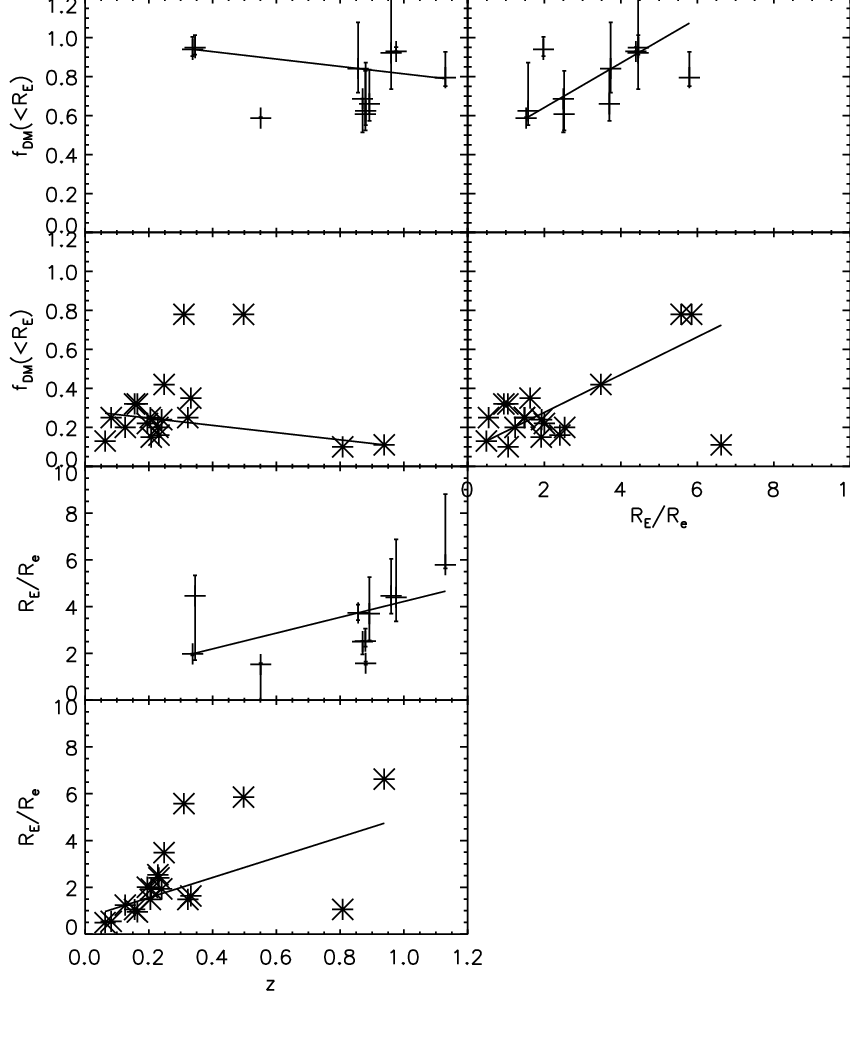
We integrate the galaxy light profile density up to the Einstein radius, and use the stellar mass of the lens galaxy, identifying the effective radius to the half stellar mass radius, to determine the stellar mass within the Einstein radius, M⋆(RE). Doing so, we can compare it to the total mass within the Einstein radius, M(RE), obtained during the lens modeling. This gives us a measurement of the lens galaxy projected DM fraction within the Einstein radius: (RE)= 1-. These values are reported in Table 7. The errors come from the propagation of the uncertainties in M⋆, Re, M(RE) and RE.
The negative DM fraction for COSMOS 0038+4133 may indicate that the stellar mass of the lens galaxy is overestimated. This is surprising as for this system the photometric and spectroscopic redshifts agree, hence making us confident that the SED, hence the stellar mass, is reliable as well. Another possible explanation is that the light profile fit is not correct and that we measure too large an effective radius. This is indeed a possible explanation as a bright ring surrounds the lens galaxy and may bias the determination of the light profile. Finally, it is also possible that the source redshift is lower than the one considered here (z=1.5). Indeed, would zs=0.9, the total mass in the Einstein radius would be M(RE)=4.881011M⊙, and the corresponding DM fraction: fDM (RE)=0.6. Because of all these interrogations, which requires further investigation, we do not keep this system for the rest of the analysis.
For the 11 remaining systems, the fraction of DM varies between 0.580.00 (COSMOS 5921+0638) and 0.95 (COSMOS 5947+4752).
In Fig. 6 we have reported the evolution of fDM (RE) with the redshift. The evolution of fDM(RE) with redshift is compatible with constant or slightly decreasing. The interpretation of this tendency is linked to the evolution of the Einstein radius, RE versus effective radius, Re. Indeed, for a given galaxy if (1) , the fraction of dark matter in the Einstein radius is expected to be “low” as, in this case, we are probing the region where the galaxy is baryon dominated: fDM(RE) is then a lower limit of the total fDM. On the contrary, if (2) : we are measuring a fDM(RE) which is getting close to the total fDM, and therefore it is expected to be larger, in average, than the one determined in case (1). This is indeed the case (see Fig 6, top right panel): fDM(RE) increases slowly when increases.
From the same Fig. 6 (bottom left panel) we see that the ratio increases quickly with redshift, meaning that as redshift grows we are measuring fDM(RE) getting closer to the total fDM of the galaxy. The fact that fDM(RE) is slightly decreasing or "at best" constant when the redshift grows suggest that the “total” fraction of dark matter is genuinely lower in high redshift lens galaxies, than in the low redshift lens galaxies.
Interestingly, we observe the same tendency if we consider the lens sample from Jiang and Kochanek (2007, JK07 hereafter): they measure the DM fraction (assuming or not adiabatic compression in their galaxy models and Salpeter initial mass function (IMF)) in the Einstein radius of 22 galaxies spanning a lens redshift =[0.0808,1.004]. If we look at the 18 galaxies with 10 as in our sample (see Fig. 6), we notice that, similarly to our sample: (i) fDM(RE) decreases slightly with redshift with the same slope than for our sample (-0.18), (ii) the radius increases with redshift and (iii) fDM(RE) slightly increases when increases.
We add that, even if the two samples show similar behavior, we chose not to mix them for the display and slope calculations in order to avoid misinterpretations due to possible systematics affecting the measurement of the DM fraction in the two different methods (e.g. different IMFs).


5 Discussion and conclusions
From the analysis of the COSMOS strong lenses in the redshift range 0.34 to 1.13, we get three major results: (1) the lens galaxy stellar masses increases with the redshift, (2) the lens galaxy environments are compatible with those of ETGs in this redshift range and (3) the DM fraction of the lens galaxies in the Einstein radius slightly decreases with the redshift, when the ratio between the Einstein radius versus the effective radius strongly increases with redshift. Let us discuss each one of these trends.
5.1 Increase of the lens stellar mass with redshift
In 2.3, we have measured that the lens galaxy stellar mass increases with redshift. Is this a result of the selection method used to built the lens sample? At z0.4, one of our lenses has an effective radius of 0.3″ and at z0.9, the smallest lens galaxy effective radius is 0.2″(see Table 5). The effective radius is a lower limit for the Einstein radius. These “lower limit Einstein radii” correspond to lower limits in mass within the Einstein radius that are in our case: 1010.9 M⊙ at z=0.4 and 1011.0 M⊙ at z=0.9, assuming a source at z=1.5. Hence, for a given source redshift, the minimal lens galaxy mass should increase with the lens redshift in order to be visually detected; hence, most probably, the minimal stellar mass might increase as well with redshift. Following this reasoning, we expect the sample average stellar mass to increase with the redshift. While this reasoning is simplistic as the source redshifts are different for every lens, it still explains partially the increasing stellar mass with increasing redshift of the lens galaxies. So far, it is not clear whether this "detection bias" effect is the only reason for the lens galaxy stellar mass increase with redshift. This result should be investigated in dedicated numerical simulations (e.g. van de Ven et al. (2009), Mandelbaum et al. (2009)).
5.2 Evolution of the lens galaxy environment
Our study of the environments of COSMOS lens galaxies, via the projected galaxy number density in 3.1, indicates that the environment of lens galaxies is similar to that of ETGs across the whole range of redshifts tested here. This result extends the previous measurements made in the redshift range [0.068; 0.513] with the SLACS sample (T09 and Auger 2008). It is particularly interesting as the COSMOS and SLACS samples have very different selection criteria: hence this result is most probably a genuine characteristic of strong lens galaxies rather than a selection bias.
We also notice that both neighbor density estimator tested here appear to be reliable estimators of the environment of galaxies, as X-ray groups and clusters are actually detected around lenses with high and high ratios.
5.3 The decreasing dark matter fraction with redshift
We have measured the lens galaxy DM fraction in the Einstein radius by combining the total mass in the Einstein radius, the light density profile and the stellar mass in the galaxy. The projected DM fraction decreases with redshift even though the ratio between the Einstein radius and the effective radius increases with the redshift (see Fig. 6). A similar trend is seen in the lens galaxy dataset of JK07 which covers a similar redshift range. Using toy models and a CDM cosmology and the SLACS lenses, Napolitano et al. (2010) and Tortora et al. (2010) first notice that, for a fixed stellar mass and age, the DM fraction is similar for high and low redshift galaxies. They also notice that the slope of the distribution of fDM versus age is steeper than explained by their model and they invoke different scenarios to interpret the discrepancy (including adiabatic compression and different IMF for different galaxy ages). Another possible effect responsible for the DM fraction decrease with redshift is the increasing stellar density of ETGs with redshift as discussed by Bezanson et al. (2009). But to understand if the results are affected by one of this effect, fDM need to be measured in comparable radius, not different for each galaxy, contrary to the Einstein radius. In order to conclude on the favorite ongoing processes on ETGs since z1 as a function of their age and stellar mass, a joint analysis of the three lens galaxy samples would certainly be a first step towards a better understanding.
5.4 Some words on the lens models
Using lens modeling we measure the Einstein radii and related total masses for the lens galaxies. Doing so, we were able to measure their DM fractions within their Einstein radius. In addition, the lens models were used to test the calculation of the external shear due to the groups around the lens galaxies. We observe that, in every lens model, the difference between the best fit external shear and the shear due to the groups points towards the closest galaxy to the lens. We calculate that, those secondary galaxies need to have realistic velocity dispersions for the lens models to provide good fits.
Moreover, we have measured that a catalog of high mass groups and clusters modeled by TIS is giving very similar total shear strengths and orientations than a combination of high mass and low mass group catalogs. Therefore we conclude that a measurement of the global external shear affecting the lens potential at the lens galaxy location could be made if one could combine : 1) a measurement of the redshift and velocity dispersion of the lens galaxy closest neighbor(s) plus 2) the locations, masses and radii of the most massive groups and clusters (such as the one provided by the X-ray observations in the COSMOS field) in a 5′ radius around the lens galaxy. By fixing the external shear one would break an important source of degeneracy in the lens models.
5.5 Conclusions
On one hand, we have measured that the environment of lens galaxies is similar to that of non ETGs over a wide redshift range: between 0.068 and 1.13 if we put together results from the SLACS sample (T09, Auger 2008) and from the COSMOS sample (this paper). On the other hand, we have built up an ensemble of clues suggesting that the mass properties of lens galaxies evolve with redshift.
Indeed, we notice that at high redshift, lens galaxies have a large stellar mass and a total dark matter fraction 0.7 (for z0.8). On the contrary, at low redshifts, lens galaxies have lower stellar mass and their DM fraction are 0.8.
This results advocates in favor of high stellar density of high redshift ETGs in comparison to low redshift ETGs as suggested by the results of Bezanson et al. (2009). Or it could be that the difference between low and high redshift lens galaxy population is a consequence of the stellar population aging and different IMFs at different ages (see Napolitano et al. 2010). It could also be that the effects measured here are related to the lensing efficiency, which in this case would be a complex combination of (1) the lens population number density, (2) the source population distribution in space, redshift and luminosity, (3) the survey properties (sensitivity, band, size, angular resolution), (4) biases in the lens sample selection.
To disentangle between an evolutionary or a pure lensing origin of the effects discovered in this study, the evolution of lens galaxy properties with redshift needs to be studied in dedicated numerical simulations (e.g. van de Ven et al. (2009), Mandelbaum et al. (2009)). Whether the effects are intrinsic to the massive early type galaxy population or to the lensing efficiency, they must be fully understood if one wants to study properly the galaxy properties gathered from lens galaxy populations.
Acknowledgements.
We acknowledge the anonymous referee for providing a detailed and very useful report. We are gratefully indebted to M. Limousin and R. Gavazzi for enlightening discussions. DA thanks CNRS and CEA for support and visits to the Geneva observatory where this work was finalized. JPK thanks support from CNRS and SL2S ANR-06-BLAN-0067 and DESIR ANR-07-BLAN-0228. E.J. acknowledges the support of the NPP, administered by Oak Ridge Associated Universities through a contract with NASA.References
- Allam et al. (2007) Allam, S. S., Tucker, D. L., Lin, H., Diehl, H. T., Annis, J., Buckley-Geer, E. J., & Frieman, J. A. 2007, ApJ, 662, L51
- Anguita et al. (2009) Anguita, T., Faure, C., Kneib, J.-P., Wambsganss, J., Knobel, C., Koekemoer, A. M., & Limousin, M. 2009, A&A, 507, 35
- Auger (2008) Auger, M.W. 2008, MNRAS, 383, L40
- Bartelmann et al. (2003) Bartelmann, M., Meneghetti, M., Perrotta, F., Baccigalupi, C., & Moscardini, L. 2003, A&A, 409, 449
- Bezanson et al. (2009) Bezanson, R., van Dokkum, P. G., Tal, T., Marchesini, D., Kriek, M., Franx, M., & Coppi, P. 2009, ApJ, 697, 1290
- Bolton et al. (2006) Bolton, A. S., Burles, S., Koopmans, L. V. E., Treu, T., & Moustakas, L. A. 2006, ApJ, 638, 703
- Bolton et al. (2008) Bolton, A. S., Burles, S., Koopmans, L. V. E., Treu, T., Gavazzi, R., Moustakas, L. A., Wayth, R., & Schlegel, D. J. 2008, ApJ, 682, 964
- Bruzual & Charlot (2003) Bruzual, G. & Charlot, S. 2003, MNRAS, 344, 1000
- Bundy et al. (2006) Bundy, K. et al. 2006, ApJ, 651, 120
- Cabanac et al. (2007a) Cabanac, R. A., et al. 2007, A&A, 461, 813
- Capak et al. (2007a) Capak, P., et al. 2007a, ApJS, 172, 99
- Capak et al. (2007b) Capak, P., Abraham, R. G., Ellis, R. S., Mobasher, B., Scoville, N., Sheth, K., & Koekemoer, A. 2007b, ApJS, 172, 284
- Capak et al. (2009) Capak, P., et al. 2009, arXiv:0910.0444
- Chae et al. (2006) Chae, K.-H., Mao, S., & Kang, X. 2006, MNRAS, 373, 1369
- Chantry & Magain (2007) Chantry, V., & Magain, P. 2007, A&A, 470, 467
- Dobke et al. (2007) Dobke, B. M., King, L. J., & Fellhauer, M. 2007, MNRAS, 377, 1503
- Elvis et al. (2009) Elvis, M., et al. 2009, ApJS, 184, 158
- Faure et al. (2008) Faure, C., et al. 2008, ApJS, 176, 19
- Faure et al. (2009) Faure, C., et al. 2009, ApJ, 695, 1233
- Finoguenov et al. (2007) Finoguenov, A., et al. 2007, ApJS, 172, 182
- Finoguenov et al. (2009) Finoguenov, A., et al. 2009, ApJ, 704, 564
- Gavazzi et al. (2007) Gavazzi, R., Treu, T., Rhodes, J. D., Koopmans, L. V. E., Bolton, A. S., Burles, S., Massey, R. J., & Moustakas, L. A. 2007, ApJ, 667, 176
- Grillo et al. (2009) Grillo, C., Gobat, R., Lombardi, M., & Rosati, P. 2009, A&A, 501, 461
- Hasinger et al. (2007) Hasinger, G., et al. 2007, ApJS, 172, 29
- Hilbert et al. (2007) Hilbert, S., White, S. D. M., Hartlap, J., & Schneider, P. 2007, MNRAS, 382, 121
- Hilbert et al. (2008) Hilbert, S., White, S. D. M., Hartlap, J., & Schneider, P. 2008, MNRAS, 386, 1845
- Ilbert et al. (2009a) Ilbert, O., et al. 2009, ApJ, 690, 1236
- Ilbert et al. (2010) Ilbert, O., et al. 2010, ApJ, 709, 644
- Jackson (2008) Jackson, N. 2008, MNRAS, 389, 1311
- Jiang & Kochanek (2007) Jiang, G., & Kochanek, C. S. 2007, ApJ, 671, 1568
- Jullo et al. (2007) Jullo, E., Kneib, J.-P., Limousin, M., Elíasdóttir, Á., Marshall, P. J., & Verdugo, T. 2007, New Journal of Physics, 9, 447
- Keeton (2001) Keeton, C. R. 2001, ApJ, 561, 46
- Keeton (2003) Keeton, C. R. 2003, ApJ, 584, 664
- Kneib et al. (1993) Kneib, J. P., Mellier, Y., Fort, B., & Mathez, G. 1993, A&A, 273, 367
- Knobel et al. (2009) Knobel, C., et al. 2009, ApJ, 697, 1842
- Kochanek (2002) Kochanek, C. S. 2002, The Shapes of Galaxies and their Dark , 62
- Koekemoer et al. (2007) Koekemoer, A. M., et al. 2007, ApJS, 172, 196
- Koopmans et al. (2006) Koopmans, L. V. E., Treu, T., Bolton, A. S., Burles, S., & Moustakas, L. A. 2006, ApJ, 649, 599
- Lagattuta et al. (2010) Lagattuta, D. J., et al. 2010, ApJ, 716, 1579
- Leauthaud et al. (2010) Leauthaud, A., et al. 2010, ApJ, 709, 97
- Lilly et al. (2007) Lilly, S. J., et al. 2007, ApJS, 172, 70
- Lilly et al. (2009) Lilly, S. J., et al. 2009, ApJS, 184, 218
- Limousin et al. (2007) Limousin, M., Kneib, J. P., Bardeau, S., Natarajan, P., Czoske, O., Smail, I., Ebeling, H., & Smith, G. P. 2007, A&A, 461, 881
- Limousin et al. (2009) Limousin, M., Sommer-Larsen, J., Natarajan, P., & Milvang-Jensen, B. 2009a, ApJ, 696, 1771
- Limousin et al. (2009) Limousin, M., et al. 2009b, A&A, 502, 445
- Mandelbaum et al. (2009) Mandelbaum, R., van de Ven, G., & Keeton, C. R. 2009, MNRAS, 1066
- Marleau & Simard (1998) Marleau, F. R., & Simard, L. 1998, ApJ, 507, 585
- McCracken et al. (2007) McCracken, H. J., et al. 2007, ApJS, 172, 314
- Mobasher et al. (2007) Mobasher, B., et al. 2007, ApJS, 172, 117
- Momcheva et al. (2006) Momcheva, I., Williams, K., Keeton, C., & Zabludoff, A. 2006, ApJ, 641, 169
- Natarajan et al. (2009) Natarajan, P., Kneib, J.-P., Smail, I., Treu, T., Ellis, R., Moran, S., Limousin, M., & Czoske, O. 2009, ApJ, 693, 970
- Napolitano et al. (2010) Napolitano, N. R., Romanowsky, A. J., & Tortora, C. 2010, MNRAS, 405, 2351
- Ofek et al. (2003) Ofek, E.O., Rix, H.-W., & Maoz, D. 2003, MNRAS, 343, 639
- Oguri et al. (2005) Oguri, M., Keeton, C. R., & Dalal, N. 2005, MNRAS, 364, 1451
- Sanders et al. (2007) Sanders, D. B., et al. 2007, ApJS, 172, 86
- Scoville et al. (2007) Scoville, N., et al. 2007, ApJS, 172, 1
- Scarlata et al. (2007a) Scarlata, N., et al. 2007a, ApJS, 172, 406
- Scarlata et al. (2007b) Scarlata, N., et al. 2007b, ApJS, 172, 494
- Simard (1998) Simard, L. 1998, Astronomical Data Analysis Software and Systems VII, 145, 108
- Taniguchi et al. (2007) Taniguchi, Y., et al. 2007, ApJS, 172, 9
- Tortora et al. (2010) Tortora, C., Napolitano, N. R., Romanowsky, A. J., & Jetzer, P. 2010, ApJ, 721, L1
- Treu et al. (2006) Treu, T., Koopmans, L. V., Bolton, A. S., Burles, S., & Moustakas, L. A. 2006, ApJ, 640, 662
- Treu et al. (2009) Treu, T., Gavazzi, R., Gorecki, A., Marshall, P. J., Koopmans, L. V. E., Bolton, A. S., Moustakas, L. A., & Burles, S. 2009, ApJ, 690, 670
- Vikhlinin et al. (2009) Vikhlinin, A., et al. 2009, ApJ, 692, 1033
- van de Ven et al. (2009) van de Ven, G., Mandelbaum, R., & Keeton, C. R. 2009, MNRAS, 1067
- Wambsganss et al. (2005) Wambsganss, J., Bode, P., & Ostriker, J. P. 2005, ApJ, 635, L1