Euler-Heisenberg Lagrangian to all orders in the magnetic field and the Chiral Magnetic Effect
Abstract
In high energy heavy ion collisions as well as in astrophysical objects like magnetars extreme magnetic field strengths are reached. Thus, there exists a need to calculate divers QED processes to all orders in the magnetic field. We calculate the vacuum polarization graph in second order of the electric field and all orders of the magnetic field resulting in a generalization of the Euler-Heisenberg Lagrangian. We perform the calculation in the effective Lagrangian approach of J. Schwinger as well as using modified Feynman rules. We find that both approaches give the same results provided that the different finite renormalization terms are taken into account. Our results imply that any quantitative explanation of the recently proposed Chiral Magnetic Effect has to take ’Strong QED’ effects into account, because these corrections are huge.
pacs
12.20.-m and 12.20.Ds1 Motivation and Introduction
Long time ago J. Schwinger derived in a seminal paper [1]
the effective non-linear Lagrangian for constant electric and magnetic
fields in all orders. Later, the exact fermion propagator in a constant magnetic field
was derived based on this work [2, 3] and used to
treat e.g. QED processes in magnetars
[4, 5, 6, 7, 8].
The latter is
important, because the observed spectra are strongly affected by
QED effects and the deduction of e.g. the magnetic field strength
reached in these objects or the structure of the accretion column
depends crucially on the quality of
these calculations.
In heavy ion collisions even far stronger magnetic
fields, of the order of
and above,
are generated for a short time period. Recently, the STAR
experiment at BNL observed correlations between charged hadrons
which can best be understood, if one assumes that topologically
non-trivial QCD effects allow for an effective, naively CP-odd coupling
of the type , see [9, 10].
This hypothetical mechanism is called Chiral Magnetic Effect (CME).
In [11] it was argued that the electric field induced by any such
effect should minimize the energy and thus is determined by the
linear term from the coupling to
and the field energy term, quadratic in .
Therefore, whatever the precise nature of the CME might be,
it will be affected strongly by pure QED effects which drastically
change the electromagnetic field energy for such strong fields.
Thus they will alter the magnitude of the induced electric field strength
and thus the size of the charged particle correlations.
These QED effects are even important for all charge correlations,
independently of whether
the CME is confirmed by future measurements or not.
In principle these calculations should take the detailed dynamics of
heavy-ion collisions into account. In the present work, however,
we only discuss the case of constant fields, which already involves
some conceptual problems.
In the CME the induced electric fields are relatively weak, roughly
of the order of , such that it is sufficient to
determine the contribution which is quadratic in but
includes all orders in .
The main technical problem we are facing is the following:
Schwinger’s elegant calculation is based on his
proper time formalism, which from the very beginning expresses
the effective Lagrangian in terms of the gauge invariant
field strength tensor . For many dynamical applications one does
need, however, the fermion propagator for which an explicit form
is given e.g. in [3]. We, therefore, reproduced the Schwinger
result also in that formalism, which was highly non-trivial and actually
required a more careful definition of the exact fermion propagator than the one given in [3].
These technical problems are also reflected by the literature. In many
papers the effective action result of Schwinger is used to analyze
specific situation beyond the weak field limit, e.g. [12].
In others the problem is discussed that its expansion in powers of the fields
leads to an asymptotic series, which is very difficult to handle
and discouraged some applications. However, it seems that this is
not a fundamental problem but just an unlucky choice of expansion
as was shown e.g. in [13]. In this paper we will therefore
avoid any expansion. This will lead us to expressions containing the
function, which indeed has an asymptotic expansion involving
Bernoulli numbers but has perfectly reasonable properties if not expanded.
In e.g. [14] it was discussed with great clarity that finite
regularisation terms have to be treated with care to avoid misinterpretations,
but that they do not pose a problem of principle. In our calculation we are
interested in higher order terms for which such problems do not occur
and adopt for the leading terms just the standard results.
The outline of this paper is as follows:
In section 2 we shall present the effective Lagrangian calculation within
the
Schwinger formalism and in section 3 we discuss the problems encountered
when trying to do the same calculations with Feynman rules.
In section 4 we will conclude and discuss our findings in the context of
the CME.
2 The calculation using Schwinger’s effective Lagrangian formalism
Schwinger’s expression for the effective Lagrangian of constant electromagnetic fields reads [1]
| (1) | |||||
where
| (2) | |||||
| (3) | |||||
| (4) |
and is the mass of the considered Dirac field, here of the electron. With
| (5) | |||||
| (6) | |||||
| (7) |
the real and imaginary parts read
| (8) | |||||
| (9) | |||||
and Eq.(1) simplifies to
| (10) | |||||
For renormalisation one has to subtract the logarithmic divergence and one has to decide on the finite renormalisation one chooses. In principle one could e.g. subtract the contribution for any fixed magnetic field . However, there is no good reason to introduce such an additional parameter. We follow Schwinger in subtracting the limiting case for vanishing magnetic field
| (11) | |||||
and thus obtain for the effective, renormalised Lagrangian of second order in and all orders in
| (12) | |||||
| (13) | |||||
| (14) | |||||
| (15) | |||||
| (16) | |||||
| (17) | |||||
The sign convention was chosen such that the contribution of e.g. to the energy density is
| (18) |
The behaviour of the potential is shown in Fig. 1 and Fig. 2.


It is easy to verify that for small fields one reproduces all contributions of second order in to the Euler-Heisenberg Lagrangian
| (19) | |||||
For the CME we are most interested in the case , i.e. in . The extension of to higher orders in is quite straight forward. For the term of interest one gets to arbitrary order
| (20) | |||||
with a numerical factor which is given in Table 1 for up to 8. It decreases approximately exponentially with the order of the expansion N. To get the corresponding terms in the energy density one has to multiply the by an additional factor of , of course, due to Eq.(18). The result can be tested again using the Euler-Heisenberg Lagrangian. For and small magnetic fields it reproduces exactly the missing term of order in Eq.(19)
| (21) | |||||
| 2 | 3 | 4 | 5 | 6 | 7 | 8 | |
|---|---|---|---|---|---|---|---|
In heavy ion collisions is much larger than such that one can use the asymptotic expansion of the function
| (22) |
For one finds , nine times the free electric field energy. Plots of the relevant quantities are shown in Fig. 3.
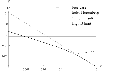
As argued in [11] this increase of the total electric field energy by a factor 10 will in turn reduce the induced electric field strength substantially. Even more important is the fact that grows linearly in , just as the driving topological term. If it had grown faster (e.g. like as for the Euler-Heisenberg Lagrangian), the CME would have died out with increasing . As it is the induced electric field is only little dependent for strong fields. However, one should keep in mind that our result applies only to the situation of constant fields, which is not a good approximation for a heavy ion collision.
3 An alternative calculation using the explicit form of the fermion propagator
Schwinger’s approach is the most efficient one, when the aim is to derive the effective higher-order photon action. However, one often wants to study dynamical quantum processes in a constant background field. To do so, one needs the modified Feynman rules in such a background field. In this section we will try to re-derive the result just obtained for with the Schwinger approach, namely the effective action in second order in the electric field and all orders in the magnetic one, using the explicit form of the fermion Feynman propagator given in [3]. This exercise is meant to demonstrate that one can actually do so, but also that special care is needed with respect to finite renormalisation terms. The propagator reads
| (23) | |||||
where an prescription was introduced such as to make a Wick rotation
in possible, which lies at the heart of this approach.
It will always make the results finite
and thus includes implicitly a regularisation. As mentioned in the
Introduction different
renormalisation schemes differ by finite renormalisation terms.
In the Geprägs et al. approach
this ambiguity might show up as an ambiguity in the choice of the
prescription, but this was not explored so far. To simplify the notation the will be suppressed from now on.
The situation is rather complicated. The function has a countably infinite number of essential singularities on the positive real axis at
| (25) |
Thus the analytic continuation is highly non-trivial and we will show that for our case this prescription leads to a different finite renormalisation than the Schwinger formula. (The leading logarithmic divergence is naturally renormalised in the same way.) Physics-wise the problem can be linked to the existence of Landau orbitals in a constant magnetic field. The Fourier transform of Eq.(23) gives typically Gaussians of the form:
| (26) |
and for e.g. one gets identical weight factors for all Landau orbits with
| (27) | |||||
| (28) |
with the anomalous magnetic moment . This can also be interpreted
more intuitively as follows: UV regularisation is concerned with the
short distance behavior. For arbitrarily small all classical Landau
orbits return to the starting point and thus give an unsuppressed contribution.
In contrast Schwinger subtracts only the contribution.
One cannot expect that the integrals from Eq.(23), the sum over
Landau orbits and the limit commute.
The Geprägs et al. result should still give the correct answer,
but only up to finite renormalization terms.
Therefore, we will
proceed as follows: we will apply this approach disregarding the
problems just discussed
and will adjust the finite regularisation terms in the final
expression to the Schwinger result. (We were not able to find an
prescription which would automatically result in an expression in the
same renormalisation scheme as Schwinger’s approach.)
Luckily, the changes to be made are rather obvious.
In any case, we find it very reassuring that
up to this finite regularisation term both approaches lead to
the same result.
We treat the magnetic field exactly, i.e. as part of and the electric field as perturbation, i.e. as part of and equate the second order of the expectation value
| (29) |
with the first order of the effective electromagnetic Lagrangian we are seeking (which is of second order in the electric field ), i.e.
| (30) |
We basically calculate the vacuum polarization graph depicted in Fig. 4 for a constant field in the background of an external constant field.

For simplicity we only discuss the case ,
most relevant for the CME.
For constant fields, rather than
point photons, the propagator from to fulfills
| (31) |
with the gauge invariant derivative rather than the usual one. This introduces an overall gauge factor, which in turn leads to covariant derivatives of the form
| (32) |
see [15]. In [16] this was actually already
discussed in connection with the CME.
We chose the 4-coordinates
,
.
The expression to be calculated is
| (33) | |||||
| (34) |
where we adopted the gauge .
With the abbreviations
| (35) | |||||
| (36) |
one gets
| (37) | |||||
| (38) | |||||
Note that the first exponentials of the propagators cancelled in Eq. (38) so that
.
Evaluating the exponentials in the trace yields
| (39) |
The evaluation of the trace is straight forward and gives
| (40) | |||||
with the notation and . Now we rotate the and integrals to the positive imaginary axis, and perform a Wick-rotation for , yielding
| (41) | |||||
After performing all Gaussian integrals this simplifies to
| (42) | |||||
which is an even function in , allowing us to substitute , by , . In terms of these variables we introduce and and perform the integration to obtain
| (43) | |||||
which differs from the result obtained in the last section
| (44) |
only in the subtracted renormalisation term. While in the Schwinger treatment the latter is independent
| (45) |
the former is not. We correct this by simply adding the relative finite renormalisation term
We conclude that the approach from Geprägs et al. can be used equally well, if the renormalisation for all loop graphs is adapted to the usual conventions.
4 Conclusions
In this publication we have calculated higher-order terms of the effective
electromagnetic Lagrangian. While strong QED is an
interesting and active field in its own right, with applications in
e.g. the astrophysics of magnetars, these studies were specifically
motivated by the Chiral Magnetic Effects (CME), possibly observed in
high-energy heavy ion collisions. The postulated mechanism is that the extremely
strong magnetic fields present in the early phase of such a collision in
combination with topological tunneling in QCD could induce an electric field,
subsequently generating specific charge correlations. For any such mechanism
strong QED effects are so large that they have to be taken into account
for any quantitative description. This was demonstrated in our paper for
the case of constant electric and magnetic fields. The observed charge
correlations are small, hinting to an electric field strength of the order
100 MeV2, while the magnetic field strength is of the order ,
such that the most relevant term is of second order in and all orders in
. We calculated this contribution.
The result we got implies that strong QED effects increase the energy density
associated with an electric field by an order of magnitude for
, thus strongly suppressing the size of such fields as
compared to naive expectations. This result is obviously most relevant
for the CME, although the approximation of constant fields is probably a
bad one for the heavy-ion setting where the fields change on time and
distance scales of several fm, which is also the radius of Landau orbits
for the fields considered. If the CME is confirmed by future experiments
at RHIC and especially LHC, where the fields will still be stronger and
even more Lorentz contracted, one will have to develop techniques to
treat also the dynamics of the strong QED effects reliably.
For calculations of e.g. Compton scattering in the accretion column of a
magnetar one needs the Feynman rules for a magnetic background field, as
given e.g. by Geprägs et al. [3]. Therefore, we performed
our calculation also with these explicit Feynman rules and showed that
the result agrees with that calculated in the Schwinger approach up
to a finite renormalisation term. We see this as an important check
for the Geprägs et al. approach, which also illustrates nicely some of
the technical problems encountered by any such calculation.
Finally, in the Schwinger approach we generalized the result to
higher orders in the field strength.
5 Acknowledgement
This work was supported by BMBF. A.S. also acknowledges the hospitality of the Yukawa Institute, Kyoto, Japan, where part of this work was done. We thank Berndt Müller and Kenji Fukushima for fruitful discussions.
References
- (1) J. Schwinger, Phys./ Rev./ 82 (1951) 664
- (2)
J. Géhéniau, Physica XVI (1950) 822
J. Géhéniau and M. Demeur, Physica XVII (1951) 71 - (3) R. Geprägs, H. Riffert, H. Herold, H. Ruder and G. Wunner, Phys. Rev. D 49 (1994) 5582.
- (4) D. Lai, W. C. G. Ho, M. van Adelsberg and J. S. Heyl, arXiv:0906.4717 [astro-ph.HE], and references therein
- (5) P. Meszaros and J. Ventura, Phys. Rev. D 19 (1979) 3565.
- (6) H. Herold, Phys. Rev. D 19 (1979) 2868.
- (7) H. Herold, H. Ruder and G. Wunner, Phys. Rev. Lett. 54 (1985) 1452.
- (8) J. S. Heyl and L. Hernquist, Mon. Not. Roy. Astron. Soc. 362 (2005) 777 [arXiv:astro-ph/0502349].
- (9) B. I. Abelev et al. [STAR Collaboration], Phys. Rev. Lett. 103 (2009) 251601 [arXiv:0909.1739 [nucl-ex]].
- (10) K. Fukushima, D. E. Kharzeev and H. J. Warringa, Phys. Rev. D 78 (2008) 074033 [arXiv:0808.3382 [hep-ph]].
- (11) A. Majumder, B. Müller, A. Schäfer, to be published.
- (12) Y. M. Cho, D. G. Pak and M. L. Walker, Phys. Rev. D 73 (2006) 065014 [arXiv:hep-th/0603031].
- (13) Y. M. Cho and D. G. Pak, Phys. Rev. Lett. 86 (2001) 1947 [arXiv:hep-th/0006057].
- (14) C. G. Beneventano and E. M. Santangelo, [arXiv:hep-th/0006123].
- (15) J. F. Nieves and P. B. Pal, Phys. Rev. D 73 (2006) 105003 [arXiv:hep-ph/0603024].
- (16) S. i. Nam, Phys. Rev. D 80 (2009) 114025 [arXiv:0911.0509 [hep-ph]].