Reformulation of the Covering and Quantizer Problems as Ground States of Interacting Particles

S. Torquato Email: torquato@electron.princeton.edu Affiliation: Department of Chemistry, Princeton University, Princeton New Jersey 08544, USA Affiliation: Department of Physics, Princeton University, Princeton New Jersey 08544, USA Affiliation: Princeton Center for Theoretical Science, Princeton University, Princeton New Jersey 08544, USA Affiliation: Program in Applied and Computational Mathematics, Princeton University, Princeton New Jersey 08544, USA Affiliation: Princeton Institute for the Science and Technology of Materials, Princeton University, Princeton New Jersey 08544, USA

August 24, 2026

Abstract

It is known that the sphere packing problem and the number variance problem (closely related to an optimization problem in number theory) can be posed as energy minimizations associated with an infinite number of point particles in $d$ -dimensional Euclidean space $\mathbb{R}^{d}$ interacting via certain repulsive pair potentials. We reformulate the covering and quantizer problems as the determination of the ground states of interacting particles in $\mathbb{R}^{d}$ that generally involve single-body, two-body, three-body, and higher-body interactions. This is done by linking the covering and quantizer problems to certain optimization problems involving the “void” nearest-neighbor functions that arise in the theory of random media and statistical mechanics. These reformulations, which again exemplifies the deep interplay between geometry and physics, allow one now to employ theoretical and numerical optimization techniques to analyze and solve these energy minimization problems. The covering and quantizer problems have relevance in numerous applications, including wireless communication network layouts, the search of high-dimensional data parameter spaces, stereotactic radiation therapy, data compression, digital communications, meshing of space for numerical analysis, and coding and cryptography, among other examples. In the first three space dimensions, the best known solutions of the sphere packing and number variance problems (or their “dual” solutions) are directly related to those of the covering and quantizer problems, but such relationships may or may not exist for $d\geq 4$ , depending on the peculiarities of the dimensions involved. Our reformulation sheds light on the reasons for these similarities and differences. We also show that disordered saturated sphere packings provide relatively thin (economical) coverings and may yield thinner coverings than the best known lattice coverings in sufficiently large dimensions. In the case of the quantizer problem, we derive improved upper bounds on the quantizer error using sphere-packing solutions, which are generally substantially sharper than an existing upper bound in low to moderately large dimensions. We also demonstrate that disordered saturated sphere packings yield relatively good quantizers. Finally, we remark on possible applications of our results for the detection of gravitational waves.

pacs

05.20.-y, 89.20.Ff, 89.70.-a, 89.75.Kd

I Introduction

There are certain scientific problems that provide deep connections between many different scientific fields. The study of the low-energy states of classical interacting many-particle systems is an exemplar of a class of such problems because of its manifest importance in physics, materials science, communication theory, cryptography, mathematics and computer science. Such many-particle systems have been used with great success to model liquids, glasses and crystals when quantum effects are negligible [1, 2]. The total potential energy $\Phi_{N}({\bf r}^{N})$ of $N$ identical particles with positions ${\bf r}^{N}\equiv{\bf r}_{1},{\bf r}_{2},\ldots,{\bf r}_{N}$ in some large volume in $d$ -dimensional Euclidean space $\mathbb{R}^{d}$ can be resolved into separate one-body, two-body, $\ldots$ , $N$ -body contributions:

\Phi_{N}({\bf r}^{N})=\sum_{i=1}^{N}u_{1}({\bf r}_{i})+\sum_{i<j}^{N}u_{2}({\bf r}_{i},{\bf r}_{j})+\sum_{i<j<k}^{N}u_{3}({\bf r}_{i},{\bf r}_{j},{\bf r}_{k})+\cdots+u_{N}({\bf r}^{N}),

(1)

where $u_{n}$ represents the intrinsic $n$ -body interaction in excess to the interaction energy for $n-1$ particles. To make the statistical-mechanical problem more tractable, the exact many-body potential (1) is usually replaced by a mathematically simpler form. For example, in the absence of an external field (i.e., $u_{1}=0$ ), often one assumes pairwise additivity, i.e.,

\Phi_{N}({\bf r}^{N})=\sum_{i<j}^{N}u_{2}({\bf r}_{i},{\bf r}_{j}).

(2)

Pairwise additivity is exact for hard-sphere systems and frequently has served to approximate accurately the interactions in simple liquids, such as the well-known Lennard-Jones pair potential [1], and in more complex systems where the pair potential $u_{2}$ in (2) can be regarded to be an effective pair interaction [3].

An outstanding problem in classical statistical mechanics is the determination of the ground states of $\Phi_{N}({\bf r}^{N})$ , which are those configurations that globally minimize $\Phi_{N}({\bf r}^{N})$ and hence are the states that exist at absolute zero temperature. While classical ground states are readily produced by slowly freezing liquids in experiments and computer simulations, our theoretical understanding of them is far from complete [4, 5]. Virtually all theoretical/computational ground-state studies of many-particle systems have been conducted for pairwise additive potentials [1, 6, 4, 7, 8, 9, 10, 11]. Often the ground states of short-range pairwise interactions are crystal structures in low dimensions [1, 6, 4, 7, 8, 9, 10, 12], but long-range interactions exist that can suppress any kind of symmetry leading to disordered ground states in low dimensions [13, 14]. Moreover, in sufficiently high dimensions, it has been suggested that even short-ranged pairwise interactions possess disordered ground states [15, 16, 17].

Ground states of purely repulsive pair interactions have profound connections not only to low-temperature states of matter but to problems in pure mathematics, including discrete geometry and number theory [18, 19, 10], information theory, and computer science. As will be explained further below, it is known that the sphere packing problem and the number variance problem (closely related to an optimization problem in number theory) can be posed as energy minimizations associated with an infinite number of point particles in $d$ -dimensional Euclidean space $\mathbb{R}^{d}$ interacting via certain repulsive pair potentials. Both of these problems can be interpreted to be optimization problems involving point processes, which can then be recast as energy minimizations. A point process in $\mathbb{R}^{d}$ is a distribution of an an infinite number of points in $\mathbb{R}^{d}$ at number density $\rho$ (number of points per unit volume) with configuration ${\bf r}_{1},{\bf r}_{2},\ldots$ ; see Ref. [16] for a precise mathematical definition.

A packing of congruent nonoverlapping spheres is a special point process in which there is a minimal pair separation distance, equal to the sphere diameter. The sphere packing problem seeks to determine the densest arrangement(s) of congruent, nonoverlapping $d$ -dimensional spheres in Euclidean space $\mathbb{R}^{d}$ [18, 20]. Although it is simple to state, it is a notoriously difficult problem to solve rigorously. Indeed, Kepler’s four-century-old conjecture, which states that the face-centered-cubic lattice in $\mathbb{R}^{3}$ is maximally dense, was only recently proved [21]. For $d\geq 4$ , the packing problem remains unsolved [18, 20, 22]. It is well known that the sphere packing problem can be posed as an energy minimization problem involving pairwise interactions between points in $\mathbb{R}^{d}$ (e.g., inverse power-law functions in which the exponent tends to infinity); see Ref. [10] and references therein.

Problems concerning the properties and quantification of density fluctuations in many-particle systems continue to provide many theoretical challenges. Of particular interest are density fluctuations that occur on some local length scale [23]. It has been shown that the minimal number variance associated with points (e.g., centroids of atomic or molecular systems) contained within some “window” can also be formulated as a ground-state problem involving bounded repulsive pair interactions with compact support [23, 24]. For spherical windows in the large-radius limit, the best known solutions in $\mathbb{R}^{d}$ are usually point configurations that are “duals” (in the sense discussed later in the paper) to the best known sphere packings in $\mathbb{R}^{d}$ .

The focus of this paper is on two other optimization problems involving point processes in $\mathbb{R}^{d}$ : the covering and quantizer problems. Roughly speaking, the covering problem asks for the point configuration that minimizes the radius of overlapping spheres circumscribed around each of the points required to cover $\mathbb{R}^{d}$ . The covering problem has applications in wireless communication network layouts [25], the search of high-dimensional data parameter spaces (e.g., search templates for gravitational waves) [26], and stereotactic radiation therapy [27]. The quantizer problem is concerned with finding the point configuration in $\mathbb{R}^{d}$ that minimizes a “distance error” associated with a randomly placed point and the nearest point of the point process. It has applications in computer science (e.g., data compression) [18], digital communications [18], coding and cryptography [28], and optimal meshing of space for numerical applications (e.g., quadrature and discretizing partial differential equations) [29]. Heretofore, the covering and quantizers problems were not known to correspond to any ground-state problems.

We reformulate the covering and quantizer problems as the determination of the ground states of interacting particles in $\mathbb{R}^{d}$ that generally involve single-body, two-body, three-body, and higher-body interactions. This is done by linking the covering and quantizer problems to certain optimization problems involving the “void” nearest-neighbor functions that arise in the theory of random media and statistical mechanics [2, 30, 31]. These reformulations, which again exemplifies the deep interplay between geometry and physics, enable one to employ theoretical and numerical optimization techniques to solve these energy minimization problems. We find that disordered saturated sphere packings (roughly, packings in which no space exists to add an additional sphere) provide relatively thin (i.e., economical) coverings and may yield thinner coverings than the best known lattice coverings in sufficiently large dimensions. In the case of the quantizer problem, we derive improved upper bounds on the quantizer error that utilize sphere-packing solutions. These improved bounds are generally substantially sharper than an existing upper bound in low to moderately large dimensions. We also demonstrate that disordered saturated sphere packings yield relatively good quantizers. Our reformulation helps to explain why the known solutions of quantizer and covering problems are identical in the first three space dimensions and why they can be different for $d\geq 4$ . In the first three space dimensions, the best known solutions of the sphere packing and number variance problems are directly related to those of the covering and quantizer problems, but such relationships may or may not exist for $d\geq 4$ , depending on the peculiarities of the dimensions involved.

We begin by summarizing basic definitions and concepts in Sec. II. Because of the connections between the sphere-packing, number-variance, covering and quantizer problems, in Sec. III, we formally define each of these problems, summarize key developments, and compare the best known solutions for each of them in selected dimensions. This includes calculations obtained for the best known number-variance solutions for $d=12,16$ and 24. We then define in Sec. IV the void nearest-neighbor functions and represent them in terms of series involving certain integrals over the $n$ -particle correlation functions, which statistically characterize an ensemble of interacting points. The special case of a single realization of the point distribution follows from this ensemble formulation, which reveals that quantizer and covering problems can be expressed as ground-state solutions of many-body interactions of the general form (1). Section V specifically gives these ground-state reformulations and shows how some known solutions in low dimensions can be explicitly recovered using the void nearest-neighbor functions. In Sec. VI, we show that disordered saturated sphere packings provide relatively thin coverings and may yield thinner coverings than the best known lattice coverings in sufficiently large dimensions. In Sec. VII, we derive improved upper bounds on the quantizer error that utilize sphere-packing solutions. We also show that disordered saturated sphere packings yield relatively good quantizers. Finally, in Sec. VIII, we make concluding remarks and comment on the application of the quantizer problem to the search for gravitational waves.

II Definitions and Preliminaries

For a statistically homogeneous point process in $\mathbb{R}^{d}$ at number density $\rho$ (number of points per unit volume), the quantity $\rho^{n}g_{n}({\bf r}_{1},{\bf r}_{2},\ldots,{\bf r}_{n})$ is proportional to the probability density for simultaneously finding $n$ sphere centers at locations ${\bf r}_{1},{\bf r}_{2},\dots,{\bf r}_{n}$ in $\mathbb{R}^{d}$ [1]. With this convention, each $n$ -particle correlation function $g_{n}$ approaches unity when all of the points become widely separated from one another. Statistical homogeneity implies that $g_{n}$ is translationally invariant and therefore only depends on the relative displacements of the positions with respect to some arbitrarily chosen origin of the system, i.e.,

g_{n}=g_{n}({\bf r}_{12},{\bf r}_{13},\ldots,{\bf r}_{1n}),

(3)

where ${\bf r}_{ij}={\bf r}_{j}-{\bf r}_{i}$ . As we will see, statistically homogeneous point processes include as special cases periodic point distributions.

The pair correlation function $g_{2}({\bf r})$ is a particularly important quantity. If the point process is also rotationally invariant (statistically isotropic), then $g_{2}$ depends on the radial distance $r\equiv|{\bf r}|$ only, i.e., $g_{2}({\bf r})=g_{2}(r)$ . Thus, it follows that the expected number of points $Z(R)$ found in a sphere of radius $R$ from a randomly chosen point of the point process, called the cumulative coordination function, is given by

Z(R)=\rho\int_{0}^{R}s_{1}(r)g_{2}(r)dr,

(4)

where

\displaystyle s_{1}(r)=\frac{2\pi^{d/2}r^{d-1}}{\Gamma(d/2)}

(5)

is the surface area of a $d$ -dimensional sphere of radius $r$ .

A lattice $\Lambda$ in $\mathbb{R}^{d}$ is a subgroup consisting of the integer linear combinations of vectors that constitute a basis for $\mathbb{R}^{d}$ and thus represents a special subset of point processes. In a lattice $\Lambda$ , the space $\mathbb{R}^{d}$ can be geometrically divided into identical regions $F$ called fundamental cells, each of which contains the just one point specified by the lattice vector

{\bf p}=n_{1}{\bf a}_{1}+n_{2}{\bf a}_{2}+\cdots+n_{d-1}{\bf a}_{d-1}+n_{d}{\bf a}_{d},

(6)

where ${\bf a}_{i}$ are the basis vectors for the fundamental cell and $n_{i}$ spans all the integers for $i=1,2,\cdots d$ . We denote by $v_{F}$ the volume of the fundamental cell. In the physical sciences, a lattice is equivalent to a Bravais lattice. Unless otherwise stated, we will use the term lattice. Every lattice has a dual (or reciprocal) lattice $\Lambda^{*}$ in which the sites of the lattice are specified by the dual (reciprocal) lattice vector ${\bf q}\cdot{\bf p}=2\pi m$ , where $m=\pm 1,\pm 2,\pm 3\cdots$ . The dual fundamental cell $F^{*}$ has volume $v_{F^{*}}=(2\pi)^{d}/v_{F}$ . This implies that the number density $\rho$ of $\Lambda$ is related to the number density $\rho_{*}$ of the dual lattice $\Lambda^{*}$ via the expression $\rho\rho_{*}=1/(2\pi)^{d}$ . A periodic point process is a more general notion than a lattice because it is is obtained by placing a fixed configuration of $N$ points (where $N\geq 1$ ) within one fundamental cell of a lattice $\Lambda$ , which is then periodically replicated. Thus, the point process is still periodic under translations by $\Lambda$ , but the $N$ points can occur anywhere in the chosen fundamental cell.

Common $d$ -dimensional lattices include the hypercubic $\mathbb{Z}^{d}$ , checkerboard $D_{d}$ and root $A_{d}$ lattices, defined, respectively, by

\mathbb{Z}^{d}=\{(x_{1},\ldots,x_{d}):x_{i}\in{\mathbb{Z}}\}\quad\mbox{for}\;d\geq 1

(7)

D_{d}=\{(x_{1},\ldots,x_{d})\in\mathbb{Z}^{d}:x_{1}+\cdots+x_{d}~~\mbox{even}\}\quad\mbox{for}\;d\geq 3

(8)

A_{d}=\{(x_{0},x_{1},\ldots,x_{d})\in\mathbb{Z}^{d+1}:x_{0}+x_{1}+\cdots+x_{d}=0\}\quad\mbox{for}\;d\geq 1

(9)

where $\mathbb{Z}$ is the set of integers ( $\ldots-3,-2,-1,0,1,2,3\ldots$ ) and $x_{1},\ldots,x_{d}$ denote the components of a lattice vector of either $\mathbb{Z}^{d}$ or $D_{d}$ and $x_{0},x_{1},\ldots,x_{d}$ denote a lattice vector of $A_{d}$ . The $d$ -dimensional lattices $\mathbb{Z}^{d}_{*}$ , $D_{d}^{*}$ and $A_{d}^{*}$ are the corresponding dual lattices; see Ref. [18] for definitions. The dual lattice $\mathbb{Z}^{d}_{*}$ is also a hypercubic lattice (even if the lattice spacing is $2\pi$ times the lattice spacing of $\mathbb{Z}^{d}$ ) and hence we say that the hypercubic lattice $\mathbb{Z}^{d}$ is equivalent (similar) to its dual lattice $\mathbb{Z}^{d}_{*}$ , i.e., $\mathbb{Z}^{d}\equiv\mathbb{Z}^{d}_{*}$ . Following Conway and Sloane [18], we say that two lattice are equivalent or similar if one becomes identical to the other by possibly a rotation, reflection and change of scale, for which we use the symbol $\equiv$ . In fact, the hypercubic lattice $\mathbb{Z}^{d}$ is characterized by the stronger property of self-duality. A self-dual lattice is one with an identical dual lattice at density $\rho=\rho_{*}=1/(2\pi)^{d/2}$ , i.e., without any rotation, reflection, or change of scale [32]. The $A_{d}$ and $D_{d}$ lattices can be regarded to be $d$ -dimensional generalizations of the face-centered-cubic (fcc) lattice because this three-dimensional lattice is defined by $A_{3}\equiv D_{3}$ . In one dimension, $A_{1}=A_{1}^{*}$ (equality meaning self-duality) are identical to the integer lattice $\mathbb{Z}^{1}=\mathbb{Z}$ . In two dimensions, $A_{2}\equiv A_{2}^{*}$ defines the triangular lattice. In three dimensions, $A_{3}^{*}\equiv D_{3}^{*}$ defines the body-centered-cubic (bcc) lattice. The $d$ -dimensional laminated lattice $\Lambda_{d}$ [18, 33] is of special interest. In dimensions 8 and 24, $\Lambda_{8}\equiv E_{8}$ , where $E_{8}$ is the self-dual root lattice, and $\Lambda_{24}$ is the self-dual Leech lattice, are remarkably symmetric and believed to be the densest sphere packings in those dimensions [22]. Thus, $E_{8}=E_{8}^{*}$ and $\Lambda_{24}=\Lambda_{24}^{*}$ . The laminated lattice $\Lambda_{16}$ , called the Barnes-Wall lattice, and the Coxeter-Todd lattice $K_{12}$ are thought to be the densest lattice packings in sixteen and twelve dimensions, respectively.

Note that for a single periodic point configuration at number density $\rho$ , the radial pair correlation function can be written as

g_{2}(r)=\sum_{i=1}^{\infty}\frac{Z_{i}}{\rho s_{1}(r_{i})}\;\delta(r-r_{i}),

(10)

where $Z_{i}$ is the coordination number at radial distance $r_{i}$ (number of points that are exactly at a distance $r=r_{i}$ from a point of the point process) such that $r_{i+1}>r_{i}$ and $\delta(r)$ is a radial Dirac delta function. For cases in which each point is equivalent to any other, which includes all lattices and some periodic point processes, the coordination numbers $Z_{i}$ are integers. For point processes for which the point are generally inequivalent, $Z_{i}$ should be interpreted as the expected coordination number and hence will generally be a non-integer. Substitution of (10) into (4) gives the coordination function for such a periodic configuration as

Z(R)=\sum_{i=1}^{M}Z_{i},

(11)

where $M$ is the smallest integer for which $r_{M+1}>R$ .

Consider any discrete set of points with position vectors $Y=\{{\bf r}_{1},{\bf r}_{2},\ldots\}$ in $\mathbb{R}^{d}$ . Associated with each point ${\bf r}_{i}\in Y$ is its Voronoi cell, ${\cal V}({\bf r}_{i})$ , which is defined to be the region of space nearer to the point at ${\bf r}_{i}$ than to any other point ${\bf r}_{j}$ in the set, i.e.,

{\cal V}({\bf r}_{i})=\{{\bf x}:|{\bf x}-{\bf r}_{i}|\leq|{\bf x}-{\bf r}_{j}|\;\mbox{for all}\;{\bf r}_{j}\in Y\}.

(12)

The Voronoi cells are convex polyhedra whose interiors are disjoint, but share common faces, and therefore the union of all of the polyhedra is the whole of $\mathbb{R}^{d}$ . This partition of space is called the Voronoi tessellation. The vertices of the Voronoi polyhedra are the points whose distance from the points $Y$ is a local maximum. While the Voronoi polyhedra of a lattice are congruent to one another, the Voronoi polyhedra of a non-Bravais lattice are not identical to one another. A hole in a lattice is a point in $\mathbb{R}^{d}$ whose distance to the nearest lattice point is a local maximum. A deep hole is one whose distance to a lattice point is a global maximum. The distance ${\cal R}_{c}$ to the deepest hole of a lattice is the covering radius and is equal to the circumradius of the associated Voronoi cell (the radius of the smallest circumscribed sphere).

In the case of the $d$ -dimensional simple cubic (hypercubic) lattice $\mathbb{Z}^{d}$ , the Voronoi cell is a hypercube and there is only one type of hole with covering radius ${\cal R}_{c}=\sqrt{d}/2$ , assuming unit number density $\rho=1$ . Figure 1 shows the Voronoi cell in the case $d=3$ as well as the corresponding Voronoi cells for the three-dimensional body-centered cubic and face-centered cubic lattices. Note that the truncated octahedron is the most spherically symmetric of the three Voronoi cells shown in Fig. 1 [34].

Refer to caption — Figure 1: (Color online) Voronoi cells in $\mathbb{R}^{3}$ for simple cubic, body-centered cubic, and face-centered cubic lattices are the cube (left), truncated octahedron (middle), and rhombic dodecahedron (right), as adapted from Ref. [2]. The truncated octahedron is composed of six square and eight regular hexagonal faces. The rhombic dodecahedron is composed of twelve rhombus-shaped faces.

A sphere packing $P$ in $d$ -dimensional Euclidean space $\mathbb{R}^{d}$ is a collection of $d$ -dimensional nonoverlapping congruent spheres. The packing density or, simply, density $\phi(P)$ of a sphere packing is the fraction of space $\mathbb{R}^{d}$ covered by the spheres. For spheres of diameter $D$ and number density $\rho$ , the density is given by

\phi=\rho v_{1}(D/2),

(13)

where

v_{1}(R)=\frac{\pi^{d/2}}{\Gamma(1+d/2)}R^{d}

(14)

is the volume of a $d$ -dimensional sphere of radius $R$ .

A packing is saturated if there is no space available to add another sphere without overlapping the existing particles. We denote the packing density of such a packing by $\phi_{s}$ . A lattice packing $P_{L}$ is one in which the centers of nonoverlapping spheres are located at the points of $\Lambda$ . Thus, the density of a lattice packing $\phi^{L}$ consisting of spheres of diameter $D$ is given by

\phi^{L}=\frac{v_{1}(D/2)}{v_{F}},

(15)

where $v_{F}$ is the volume of a fundamental cell. A periodic packing of congruent spheres is obtained by placing a fixed configuration of $N$ sphere centers (where $N\geq 1$ ) within one fundamental cell of a lattice $\Lambda$ , which is then periodically replicated without overlaps. The packing density of a periodic packing is given by

\phi=\frac{Nv_{1}(D/2)}{v_{F}}=\rho v_{1}(D/2),

(16)

where $\rho=N/v_{F}$ is the number density.

III Problem Statements and Background

III.1 Sphere Packing Problem

The sphere packing problem seeks to answer the following question: Among all packings of congruent spheres, what is the maximal packing density $\phi_{\mbox{\scriptsize max}}$ , i.e., largest fraction of $\mathbb{R}^{d}$ covered by the spheres, and what are the corresponding arrangements of the spheres [35, 18]? More precisely, the maximal density is defined by

\phi_{\mbox{\scriptsize max}}=\sup_{P\subset\mathbb{R}^{d}}\phi(P),

(17)

where the supremum is taken over all packings in $\mathbb{R}^{d}$ . The sphere packing problem is of great fundamental and practical interest, and arises in a variety of contexts, including classical ground states of matter in low dimensions [6], the famous Kepler conjecture for $d=3$ [21], error-correcting codes [36, 18] and spherical codes [18].

The optimal solutions are known only for the first three space dimensions [21]. For $4\leq d\leq 9$ , the densest known packings are Bravais lattice packings [18]. For example, the “checkerboard” lattice $D_{d}$ , which is the $d$ -dimensional generalization of the fcc lattice (densest packing in $\mathbb{R}^{3}$ ), is believed to be optimal in $\mathbb{R}^{4}$ and $\mathbb{R}^{5}$ . The remarkably symmetric self-dual $E_{8}$ and Leech lattices in $\mathbb{R}^{8}$ and $\mathbb{R}^{24}$ , respectively, are most likely the densest packings in these dimensions [22]. Table 1 summarizes the densest known packings in selected dimensions.

Table 1: Best known solutions to the sphere packing problem in selected dimensions; see Conway and Sloane [18] for details.

Dimension, $d$	Packing	Packing density, $\phi$
1	$A_{1}^{*}={\mathbb{Z}}$	1
2	$A_{2}^{*}\equiv A_{2}$	$\pi/\sqrt{12}=0.906899\ldots$
3	$A_{3}\equiv D_{3}$	$\pi/\sqrt{18}=0.740480\ldots$
4	$D_{4}\equiv D_{4}^{*}$	$\pi^{2}/16=0.616850\ldots$
5	$D_{5}$	$2\pi^{2}/(30\sqrt{2})=0.465257\ldots$
6	$E_{6}$	$3\pi^{3}/(144\sqrt{3})=0.372947\ldots$
7	$E_{7}$	$\pi^{3}/105=0.295297\ldots$
8	$E_{8}=E_{8}^{*}$	$\pi^{4}/384=0.253669\ldots$
9	$\Lambda_{9}$	$\sqrt{2}\pi^{4}/945=0.145774\ldots$
10	$P_{10c}$	$\pi^{5}/3072=0.099615\ldots$
12	$\Lambda^{max}_{12}$	$\pi^{6}/23040=0.041726\ldots$
16	$\Lambda_{16}$	$\pi^{8}/645120=0.014708\ldots$
24	$\Lambda_{24}=\Lambda_{24}^{*}$	$\pi^{24}/479001600=0.001929\ldots$

For large $d$ , the best that one can do theoretically is to devise upper and lower bounds on $\phi_{\mbox{\scriptsize max}}$ [18, 20, 16]. For example, Minkowski [37] proved that the maximal density $\phi^{L}_{\mbox{\scriptsize max}}$ among all Bravais lattice packings for $d\geq 2$ satisfies the lower bound

\phi^{L}_{\mbox{\scriptsize max}}\geq\frac{\zeta(d)}{2^{d-1}},

(18)

where $\zeta(d)=\sum_{k=1}^{\infty}k^{-d}$ is the Riemann zeta function. It is seen that for large values of $d$ , the asymptotic behavior of the nonconstructive Minkowski lower bound is controlled by $2^{-d}$ . Note that the density of a saturated packing of congruent spheres in $\mathbb{R}^{d}$ for all $d$ satisfies

\phi\geq\frac{1}{2^{d}},

(19)

which has the same dominant exponential term as (18). This is a rather weak lower bound on the density of saturated packings because there exists a disordered but unsaturated packing construction in $\mathbb{R}^{d}$ , known as the “ghost” RSA packing [15], that achieves the density $2^{-d}$ in any dimension. We will employ these results in Sec. VII.2. It is also known that there are saturated packings in $\mathbb{R}^{d}$ with densities that exceed the scaling $2^{-d}$ [38], as we will discuss in Sec. III.3. In the large-dimensional limit, Kabatiansky and Levenshtein [39] showed that the maximal density is bounded from above according to the asymptotic upper bound

\phi_{\mbox{\scriptsize max}}\leq\frac{1}{2^{0.5990\,d}}.

(20)

We will employ sphere-packing solutions to obtain heretofore unattained results for both the covering and quantizer problems. In particular, we obtain coverings and quantizers utilizing disordered saturated packings in Secs. VI and VII.3, respectively. In Sec. VII, we use the densest lattice packings to derive improved upper bounds on the quantizer error.

III.2 Number Variance Problem, Hyperuniformity and Epstein Zeta Function

We denote by $\sigma^{2}(A)$ the variance in the number of points $N(A)$ contained within a window $A\subset\mathbb{R}^{d}$ . The number variance $\sigma^{2}(A)$ for a specific choice of $A$ is necessarily a positive number and is generally related to the total correlation function $h({\bf r})=g_{2}({\bf r})-1$ for a translationally invariant point process [23], where $g_{2}$ is the pair correlation function defined in Sec. II. In the special case of a spherical window of radius $R$ in $\mathbb{R}^{d}$ , the number variance is explicitly given by

\displaystyle\sigma^{2}(R)=\rho v_{1}(R)\Bigg[1+\rho\int_{\mathbb{R}^{d}}h({\bf r})\alpha(r;R)\,d{\bf r}\Bigg],

(21)

$\alpha(r;R)$ is the dimensionless volume common to two spherical windows of radius $R$ (in units of the volume of a spherical window of radius $R$ , $v_{1}(R)$ ) whose centers are separated by a distance $r$ . We will call $\alpha(r;R)$ the scaled intersection volume, which will play an important role in this paper. The scaled intersection volume has the support $[0,2R]$ , the range $[0,1]$ , and the following alternative integral representation [16]:

\displaystyle\alpha(r;R)=c(d)\int_{0}^{\cos^{-1}[r/(2R)]}\sin^{d}(\theta)\,d\theta,

(22)

where $c(d)$ is the $d$ -dimensional constant given by

\displaystyle c(d)=\frac{2\Gamma(1+d/2)}{\pi^{1/2}\Gamma[(d+1)/2]}.

(23)

Torquato and Stillinger [16] found the following series representation of the scaled intersection volume $\alpha(r;R)$ for $r\leq 2R$ and for any $d$ :

\displaystyle\alpha(r;R)=1-c(d)x+c(d)\sum_{n=2}^{\infty}(-1)^{n}\frac{(d-1)(d-3)\cdots(d-2n+3)}{(2n-1)[2\cdot 4\cdot 6\cdots(2n-2)]}x^{2n-1},

(24)

where $x=r/(2R)$ . For even dimensions, relation (24) is an infinite series because it involves transcendental functions, but for odd dimensions, the series truncates such that $\alpha(r;R)$ is a univariate polynomial of degree $d$ . For example, in two and three dimensions, respectively, the scaled intersection volumes are given by

\alpha(r;R)=\frac{2}{\pi}\left[\cos^{-1}\left(\frac{r}{2R}\right)-\frac{r}{2R}\left(1-\frac{r^{2}}{4R^{2}}\right)^{1/2}\right]\Theta(2R-r)\quad(d=2),

(25)

\alpha(r;R)=\left[1-\frac{3}{4}\frac{r}{R}+\frac{1}{16}\left(\frac{r}{R}\right)^{3}\right]\Theta(2R-r)\quad(d=3),

(26)

where

\Theta(x)=\Bigg\{{0,\quad x<0,\atop{1,\quad x\geq 0,}}

(27)

is the Heaviside step function. Figure 2 provides plots of $\alpha(r;R)$ as a function of $r$ for the first five space dimensions. For any dimension, $\alpha(r;R)$ is a monotonically decreasing function of $r$ . At a fixed value of $r$ in the interval $(0,2R)$ , $\alpha(r;R)$ is a monotonically decreasing function of the dimension $d$ .

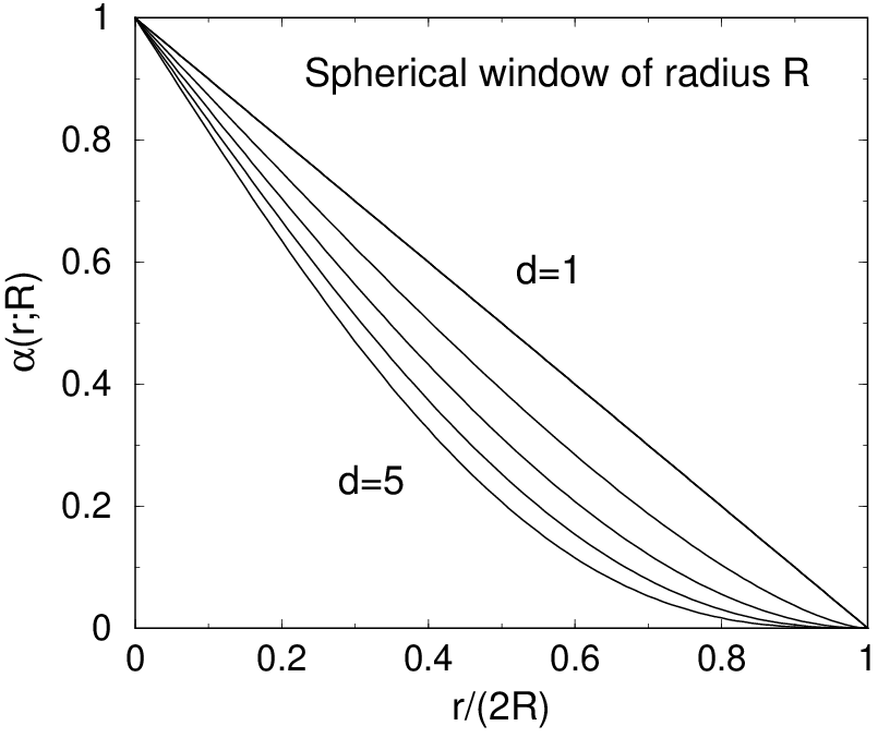
For large $R$ , it has been proved that $\sigma^{2}(R)$ cannot grow more slowly than $\gamma R^{d-1}$ , where $\gamma$ is a positive constant [40]. We note that point processes (translationally invariant or not) for which $\sigma^{2}(R)$ grows more slowly than the window volume (i.e., as $R^{d}$ ) for large $R$ are examples of hyperuniform (or superhomogeneous) point patterns [23]. For hyperuniform point processes in which the number variance grows like the surface area of the window, one has

\sigma^{2}(R)=2^{d}\eta\left[B\left(\frac{R}{{\cal D}}\right)^{d-1}+{\cal O}\left(\frac{R}{{\cal D}}\right)^{d-2}\right]\qquad R\rightarrow\infty,

(28)

where

B=\frac{\eta\;c(d)}{2{\cal D}v_{1}({\cal D}/2)}\int_{\mathbb{R}^{d}}h({\bf r})rd{\bf r},

(29)

is a dimensionless constant with $c(d)$ defined by (23),

\eta=\rho v_{1}({\cal D}/2)

(30)

is a dimensionless density, and ${\cal D}$ represents some “microscopic” length scale, such as the minimum pair separation distance in a packing or the mean nearest-neighbor distance. This class of hyperuniform point processes includes all periodic point patterns, quasicrystals that possess Bragg peaks, and disordered hyperuniform point patterns in which the pair correlation functions decay exponentially fast to unity [23].

It has been shown that finding the point process that minimizes the number variance $\sigma^{2}(R)$ is equivalent to finding the ground state of a certain repulsive pair potential with compact support [23]. Specifically, by invoking a volume-average interpretation of the number variance problem valid for a single realization of a point process, Torquato and Stillinger found [23]:

\displaystyle\sigma^{2}(R)=2^{d}\eta B_{N}(R)\left(\frac{R}{{\cal D}}\right)^{d-1},

(31)

where

B_{N}(R)=\frac{R}{{\cal D}}\left[1-2^{d}\eta\left(\frac{R}{{\cal D}}\right)^{d}+\frac{1}{N}\sum_{i\neq j}^{N}\alpha(r_{ij};R)\right].

(32)

The asymptotic coefficient $B$ defined by (29) for a hyperuniform point pattern is then related to $B_{N}(R)$ by the expression

B=\lim_{L\rightarrow+\infty}\frac{1}{L}\int_{0}^{L}B_{N}(R)dR.

(33)

These results imply that the asymptotic coefficient $B$ obtained in (29) involves an average over small-scale fluctuations in the number variance with length scale on the order of the mean separation between points [23]. In the special case of a (Bravais) lattice $\Lambda$ , one can express the rescaled surface-area coefficient as follows:

\displaystyle\eta^{1/d}B=\frac{\pi^{(d-1)/2}2^{d-1}\left[\Gamma(1+d/2)\right]^{1-1/d}}{v_{F}^{1+1/d}}\sum_{\mathbf{q}\neq\mathbf{0}}\frac{1}{\|\mathbf{q}\|^{d+1}},

(34)

where we recall that $v_{F}$ is the volume of the fundamental cell of the lattice $\Lambda$ and ${\bf q}$ represents a lattice vector in the dual (or reciprocal) lattice $\Lambda^{*}$ . The rescaled coefficient $\eta^{1/d}B$ renders the result independent of the length scale in the lattice [23].

Finding the lattice that minimizes $B$ is directly related to an outstanding problem in number theory, namely, finding the minima of the Epstein zeta function $Z_{\Lambda}(s)$ [19] defined by

Z_{\Lambda}(s)=\sum_{\bf p\neq{\bf 0}}\frac{1}{\|{\bf p}\|^{2s}},

(35)

where ${\bf p}$ is a lattice vector of the lattice $\Lambda$ . Note that the dual of the lattice that minimizes the Epstein zeta function at $s=(d+1)/2$ among all lattices will minimize the scaled asymptotic number-variance coefficient (34) among lattices [23, 41]. Certain duality relations have been derived that establish rigorous upper bounds on the energies of such ground states and help to identify energy-minimizing lattices [5]. Because $Z_{\Lambda}(s)$ is globally minimized for $d=1$ by the integer lattice [23] and is minimized for $d=2$ among all lattices by the triangular lattice [42], it has been conjectured that the Epstein zeta function for $s>0$ is minimized among lattices by the maximally dense lattice packing [43, 44]. Sarnak and Strömbergsson [19] have proved that the conjecture cannot be generally true, but for $d=4$ , $8$ and $24$ , the densest lattice packing is a strict local minimum. Since as $s\rightarrow+\infty$ , the minimizer of Epstein zeta function is the densest sphere packing in $\mathbb{R}^{d}$ for any $d$ , it is likely that in the high-dimensional limit the minimizers of this function are non-lattices, namely, disordered sphere packings [16].

Table 2: Best known solutions to the asymptotic number variance problem in selected dimensions. Values reported for

d=1,2

and 3 and

d=4

-8 are taken from Torquato and Stillinger [23] and Zachary and Torquato [41], respectively. Values reported for

d=12,16

and 24 have been determined in the present work.

Dimension, $d$	Structure	Scaled Coefficient, $\eta^{1/d}B$
1	$A_{1}^{*}=\mathbb{Z}$	0.083333
2	$A_{2}^{*}\equiv A_{2}$	0.12709
3	$A_{3}^{}\equiv D_{3}^{}$	0.15560
4	$D_{4}^{*}\equiv D_{4}$	0.17488
5	$\Lambda_{5}^{2*}$	0.19069
6	$E_{6}^{*}$	0.20221
7	$D_{7}^{+}$	0.21037
8	$E_{8}^{*}=E_{8}=D_{8}^{+}$	0.21746
12	$K_{12}^{*}\equiv K_{12}$	0.24344
16	$\Lambda_{16}^{*}\equiv\Lambda_{16}$	0.25629
24	$\Lambda_{24}^{*}=\Lambda_{24}$	0.26775

In Table 2, we tabulate the best known solutions to the asymptotic number variance problem in selected dimensions. Values for the first three space dimensions were given in Ref. [23] and those for $d=4-8$ were provided in Ref. [41]. The values reported for $d=12,16$ and 24 were ascertained using efficient algorithms based on alternative number-theoretic representations of the Epstein zeta function $Z_{\Lambda}(s)$ [19] for the corresponding densest known lattice packings for $s=(d+1)/2$ and then using the duality relations connecting it to the asymptotic surface-area coefficient for the number variance. Appendix A provides details for these computations.

III.3 Covering Problem

Surround each of the points of a point process $\cal P$ in $\mathbb{R}^{d}$ by congruent overlapping spheres of radius $R$ such that the spheres cover the space. The covering density $\theta$ is defined as follows:

\theta=\rho v_{1}(R),

(36)

where $v_{1}(R)$ is given by (14). The covering problem asks for the arrangement of points with the least density $\theta$ . We define the covering radius ${\cal R}_{c}$ for any configuration of points in $\mathbb{R}^{d}$ to be the minimal radius of the overlapping spheres to cover $\mathbb{R}^{d}$ . Figure 3 shows two examples of coverings in the plane.

The covering density associated with $A_{d}^{*}$ at unit number density $\rho=1$ is known exactly for any dimension $d$ [18]:

\theta=v_{1}(1)\sqrt{d+1}\left[\frac{d(d+2)}{12(d+1)}\right]^{d/2}.

(37)

For the hypercubic lattice $\mathbb{Z}^{d}$ at $\rho=1$ ,

\theta=v_{1}(1)\frac{d^{d/2}}{2^{d}}.

(38)

Thus the ratio of the covering density for $A_{d}^{*}$ to that of $\mathbb{Z}^{d}$ is given by

\frac{\theta(A_{d}^{*})}{\theta(Z^{d})}=\frac{\sqrt{d+1}}{3^{d/2}}\left[\frac{d+2}{d+1}\right]^{d/2}.

(39)

For large $d$ , this ratio becomes

\frac{\theta(A_{d}^{*})}{\theta(Z^{d})}\sim\frac{\sqrt{de}}{3^{d/2}},

(40)

and thus we see that $A_{d}^{*}$ provides exponentially thinner coverings than that of $\mathbb{Z}^{d}$ in the large- $d$ limit. We note that in this asymptotic limit,

\theta(A_{d}^{*})\sim\left(\frac{e}{\pi}\right)^{1/2}\left(\frac{e\pi}{6}\right)^{1/2}=0.8652559792\ldots(1.193016780\ldots)^{d}.

(41)

Until recently, $A_{d}^{*}$ was the best known lattice covering in all dimensions $d\leq 23$ . However, for most dimensions in the range $6\leq\theta\leq 15$ , Schürmann and Vallentin [45] have discovered other lattice coverings that are slightly thinner than those for $A_{d}^{*}$ . Table 3 provides the best known solutions to the covering problem in selected dimensions.

Table 3: Best known solutions to the covering problem in selected dimensions. Values reported are taken from Conway and Sloane [18], except for

d=7,8

and 9, which were obtained from Schürmann and Vallentin [45]. It is only in one and two dimensions that these solutions have been proved to be globally optimal [18].

Dimension, $d$	Covering	Covering Density, $\theta$
1	$A_{1}^{*}=\mathbb{Z}$	1
2	$A_{2}^{*}\equiv A_{2}$	1.2092
3	$A_{3}^{}\equiv D_{3}^{}$	1.4635
4	$A_{4}^{*}$	1.7655
5	$A_{5}^{*}$	2.1243
6	$L_{6}^{c1}$	2.4648
7	$L_{7}^{c}$	2.9000
8	$L_{8}^{c}$	3.1422
9	$A^{5}_{9}$	4.3401
10	$A^{*}_{10}$	5.2517
12	$A^{*}_{12}$	7.5101
16	$A^{*}_{16}$	15.3109
17	$A^{*}_{17}$	18.2878
18	$A^{*}_{18}$	21.8409
24	$\Lambda_{24}=\Lambda_{24}^{*}$	7.9035

Until the present work, there were no known explicit non-lattice constructions possessing covering densities smaller than those of the best lattice coverings in any dimension $d$ [18]. In Sec. VII, we provide evidence that certain disordered point patterns give thinner coverings than the best known lattice coverings beginning at $d=17$ . There is a fundamental difference between coverings associated with point patterns that have identical Voronoi cells (i.e., lattices and periodic point patterns in which each point is equivalent) and those point processes whose Voronoi cells are generally different (e.g., irregular point processes). This salient point is illustrated in Fig. 4 and explained in the corresponding caption.

Rogers showed that (possibly nonlattice) coverings exist with

\theta\leq 5d+d\ln(d)+d\ln(\ln(d)).

(42)

for $d\geq 2$ . This is a nonconstructive upper bound. This upper bound provides a substantially thinner covering density than that of the $A_{d}^{*}$ lattice in the large- $d$ limit [cf. (41)], but it is not known whether this bound becomes sharp in the large- $d$ limit.

The best lower bound on the covering density is given by

\theta\geq\tau_{d}.

(43)

To define $\tau_{d}$ , let $S$ be a regular simplex with edge length equal to two. Spheres of radius $\sqrt{2d/(d+1)}$ centered at the vertices of $S$ just cover $S$ . The quantity $\tau_{d}$ is the ratio of the sums of the intersections of these spheres with $S$ to the volume of $S$ . Thus, in the large- $d$ limit, $\tau\rightarrow d/e^{3/2}$ .

III.4 Quantizer Problem

Consider a point process ${\cal P}$ in $\mathbb{R}^{d}$ with configuration ${\bf r}_{1},{\bf r}_{2},\ldots,{\bf r}_{N}$ . A $d$ -dimensional quantizer is device that takes as an input a point at position ${\bf x}$ in $\mathbb{R}^{d}$ generated from some probability density function $p({\bf x})$ and outputs the nearest point ${\bf r}_{i}$ of the point process to $\bf x$ . Equivalently, if the input $\bf x$ belongs to the Voronoi cell ${\cal V}({\bf r}_{i})$ , the output is ${\bf r}_{i}$ (see Fig. 5) For simplicity, we assume that $\bf x$ is uniformly distributed over a large ball in $\mathbb{R}^{d}$ containing the $N$ points of the point process. One attempts to choose the configuration ${\bf r}_{1},{\bf r}_{2},\ldots,{\bf r}_{N}$ of the point process to minimize the mean squared error, i.e., the expected value of $|{\bf x}-{\bf r}_{i}|^{2}$ . Specifically, the quantizer problem is to choose the $N$ -point configuration so as to minimize the scaled dimensionless error (sometimes called the distortion) [18]

{\cal G}=\frac{1}{d}\langle R^{2}\rangle,

(44)

where

\langle R^{2}\rangle=\frac{\displaystyle\lim_{N\rightarrow\infty}\frac{1}{N}\sum_{i=1}^{N}\int_{{\cal V}({\bf r}_{i})}|{\bf x}-{\bf r}_{i}|^{2}d{\bf x}}{\displaystyle\langle V({\cal V})\rangle^{1+\frac{2}{d}}}.

(45)

is a dimensionless error,

\langle V({\cal V})\rangle=\displaystyle\left[\lim_{N\rightarrow\infty}\frac{1}{N}\sum_{i=1}^{N}V({\cal V}({\bf r}_{i}))\right]

(46)

is the expected volume of a Voronoi cell, and $V({\cal V}({\bf r}_{i}))$ is the volume of the $i$ th Voronoi cell. The scaling factor $1/d$ is included to compare the second moments appropriately across dimensions. We will denote the minimal scaled dimensionless error by ${\cal G}_{min}$ . Note that since there is one point per Voronoi cell, the number density $\rho$ is set equal to unity.

If all of the Voronoi cells are congruent (as they are in the case of all lattices and some periodic point processes), we have the simpler expression

{\cal G}=\frac{\frac{\displaystyle 1}{\displaystyle d}\int_{{\cal V}}|{\bf x}|^{2}d{\bf x}}{V({\cal V})^{1+\frac{2}{d}}},

(47)

where the centroid of the Voronoi cell $\cal V$ is the origin of the coordinate system. The lattice quantizer problem is to find the lattice for which $\cal G$ , given by (47), is minimum. Thus, $\cal G$ can be interpreted as the scaled, dimensionless second moment of inertia of the Voronoi cell.

Table 4: Best known solutions to the quantizer problem in selected dimensions. Values reported are taken from Conway and Sloane [18], except for

d=9

and 10, which were obtained from Agrell and Eriksson [47]. It is only in one and two dimensions that these solutions have been proved to be globally optimal [18].

Dimension, $d$	Quantizer	Scaled Error, $\cal G$
1	$A_{1}^{*}=\mathbb{Z}$	0.083333
2	$A_{2}^{*}\equiv A_{2}$	0.080188
3	$A_{3}^{}\equiv D_{3}^{}$	0.078543
4	$D_{4}^{*}\equiv D_{4}$	0.076603
5	$D_{5}*$	0.075625
6	$E_{6}^{*}$	0.074244
7	$E_{7}^{*}$	0.073116
8	$E_{8}^{*}=E_{8}$	0.071682
9	$L^{AE}_{9}$	0.071626
10	$D^{+}_{10}$	0.070814
12	$K_{12}^{*}\equiv K_{12}$	0.070100
16	$\Lambda_{16}^{*}\equiv\Lambda_{16}$	0.068299
24	$\Lambda_{24}^{*}=\Lambda_{24}$	0.065771

The best known quantizers in any dimension $d$ are usually lattices that are the duals of the densest known packings (see the discussion in Sec. III.1 and Ref. [18]), except in dimensions 9 and 10, where the best solutions are still lattices, but are not duals of the densest lattice packings in those dimensions. Although the best known solutions of the quantizer and covering problems are the same in the first three space dimensions, they are generally different for $d\geq 4$ [18, 45]. Zador [46] has derived upper and lower bounds on ${\cal G}_{min}$ . Conway and Sloane [18] have obtained conjectural lower bounds on ${\cal G}_{min}$ . We defer the discussion of these bounds to Sec. VII, where we derive sharper upper bounds on ${\cal G}_{min}$ , among other results. Table 4 provides the best known solutions to the quantizer problem in selected dimensions.

III.5 Comparison of the Four Problems

Table 5 lists the best known solutions of the quantizer, covering and number-variance problems and sphere-packing problems in $\mathbb{R}^{d}$ for selected $d$ . It is seen that in the first two space dimensions, the best known solutions for each of these four problems are identical to one another. For $d=3$ , the densest sphere packing is the $D_{3}$ or, equivalently, $A_{3}$ lattice, which is the dual lattice associated with the best known solutions to the quantizer, covering and number-variance problems, which is the $A_{3}^{*}$ lattice. Thus, for the first three space dimensions, the best known solutions for each of the four problems are lattices, and either they are identical to one another or are duals of one another. However, such relationships may or may not exist for $d\geq 4$ , depending on the peculiarities of the dimensions involved.

Table 5: Comparison of the best known solutions to the quantizer, covering, number variance and sphere packing problems, as obtained from the previous four tables. Recall that the

E_{8}

and

\Lambda_{24}

lattices are self-dual lattices.

Dimension, $d$	Quantizer	Covering	Variance	Packing
1	$A_{1}^{*}=\mathbb{Z}$	$A_{1}^{*}=\mathbb{Z}$	$A_{1}^{*}=\mathbb{Z}$	$A_{1}^{*}=\mathbb{Z}$
2	$A_{2}^{*}\equiv A_{2}$	$A_{2}^{*}\equiv A_{2}$	$A_{2}^{*}\equiv A_{2}$	$A_{2}^{*}\equiv A_{2}$
3	$A_{3}^{}\equiv D_{3}^{}$	$A_{3}^{}\equiv D_{3}^{}$	$A_{3}^{}\equiv D_{3}^{}$	$A_{3}\equiv D_{3}$
4	$D_{4}^{*}\equiv D_{4}$	$A_{4}^{*}$	$D_{4}^{*}\equiv D_{4}$	$D_{4}^{*}\equiv D_{4}$
5	$D_{5}^{*}$	$A_{5}^{*}$	$\Lambda_{5}^{2*}$	$D_{5}$
6	$E_{6}^{*}$	$L_{6}^{c1}$	$E_{6}^{*}$	$E_{6}$
7	$E_{7}^{*}$	$L_{7}^{c}$	$\Lambda_{7}^{3*}$	$E_{7}$
8	$E_{8}$	$L_{8}^{c}$	$E_{8}$	$E_{8}$
9	$L^{AE}_{9}$	$A^{5}_{9}$	$\Lambda^{*}_{9}$	$\Lambda_{9}$
10	$D^{+}_{10}$	$A^{*}_{10}$	$\Lambda^{*}_{10}$	$P_{10c}$
12	$K_{12}$	$A^{*}_{12}$	$\Lambda^{max*}_{12}$	$\Lambda^{max}_{12}$
16	$\Lambda^{*}_{16}$	$A^{*}_{16}$	$\Lambda^{*}_{16}$	$\Lambda_{16}$
24	$\Lambda_{24}$	$\Lambda_{24}$	$\Lambda_{24}$	$\Lambda_{24}$

There is a fundamental difference between the nature of the interactions for the sphere-packing problem and those for the other three problems. Any sphere packing (optimal or not) consisting of nonoverlapping spheres of diameter $D$ is described by a short-ranged pair potential that is zero whenever the spheres do not overlap (when the pair separation distance is greater than $D$ ) and is infinite whenever the pair separation distance is less than $D$ . By contrast, the other three problems are described by “soft” bounded interactions. In particular, we have seen that the number variance is specified by a bounded repulsive pair potential with compact support [cf. (31)]. We will see in the subsequent sections that the covering and quantizer problems are described by many-particle bounded interactions but of the more general form (1), which involves single-body, two-body, three-body, and higher-body interactions.

One simple reason why the optimal solutions of the sphere-packing and number-variance problems are related to one another either directly or via their dual solutions in the first three space dimensions is that they both involve short-ranged repulsive pair interactions only. The reader is referred to Refs. [23] and [5] for a comprehensive explanation. The reasons why the optimal solutions to these two problems are sometimes the optimal solutions for the covering and quantizer problems will become apparent in the subsequent sections. The explanation for why the optimal covering and quantizer solutions are generally different for $d\geq 4$ is discussed in Sec. V. We note that the Leech lattice $\Lambda_{24}$ for $d=24$ is an exceptional case in that it provides the optimal solution to all four different problems. The remarkably high degree of symmetry possessed by this self-dual lattice [22] accounts for this unique property. The only other dimensions where all four optimal solutions are the same are $d=1$ and $d=2$ .

IV Nearest-Neighbor Functions

IV.1 Definitions

We recall the definition of the “void” nearest-neighbor probability density function $H_{V}(R)$ [2]:

\displaystyle\begin{array}[]{ccp{3.7in}}H_{V}(R)\,dR&=&Probability that a point of the point process lies at a distance between $R$ and $R+dR$ from a randomly chosen point in $\mathbb{R}^{d}$.\end{array}

The “void” exclusion probability $E_{V}(R)$ is the complementary cumulative distribution function associated with $H_{V}(R)$ :

\displaystyle E_{V}(R)=\int_{R}^{\infty}H_{V}(x)dx,

(50)

and hence is a monotonically decreasing function of $R$ [2]. Thus, $E_{V}(R)$ has the following probabilistic interpretation:

\displaystyle\begin{array}[]{ccp{3.7in}}E_{V}(R)&=&Probability of finding a randomly placed spherical cavity of radius $R$ empty of any points.\end{array}

There is another interpretation of $E_{V}$ that involves circumscribing spheres of radius $R$ around each point in a realization of the point process. It immediately follows that $E_{V}(R)$ is the expected fraction of space not covered by these circumscribing spheres. Differentiating (50) with respect to $R$ gives

\displaystyle H_{V}(R)=-\frac{\partial E_{V}}{\partial R}.

(53)

Note that these void quantities are different from the “particle” nearest-neighbor functions [31, 48, 49] in which the sphere of radius $R$ is centered at an actual point of the point process (as opposed to an arbitrary point in the space).

It is useful to introduce the “conditional” nearest-neighbor function $G_{V}(r)$ [30, 31], which is defined in terms of $H_{V}(r)$ and $E_{V}(r)$ as follows:

\displaystyle H_{V}(R)=\rho s_{1}(R)G_{V}(R)E_{V}(R),

(54)

where $s_{1}(R)$ is the surface area of a $d$ -dimensional sphere of radius $R$ [cf. (5)]. Thus, we have the following interpretation of the conditional function:

\displaystyle\begin{array}[]{ccp{3.1in}}\rho s_{1}(R)G_{V}(R)\;dR&=&Given that a spherical cavity of radius $R$ centered at an arbitrary point in the space is empty of any points of the point process, the probability of finding a point in the spherical shell of volume $s_{1}(R)\,dR$ surrounding the arbitrary point.\end{array}

Therefore, it follows from (53) and (54) that the exclusion probability can be expressed in terms of $G_{V}$ via the relation

\displaystyle E_{V}(R)=\exp\left[-\rho s_{1}(1)\int_{0}^{R}x^{d-1}G_{V}(x)\;dx\right].

(57)

It is clear that the void functions have the following behaviors at the origin for $d\geq 2$ [50]:

\displaystyle E_{V}(0)=1,\qquad H_{V}(0)=0,\qquad G_{V}(0)=1.

(58)

Moments of the nearest-neighbor function $H_{V}(R)$ arise in rigorous bounds for transport properties of random media [2]. The $n$ th moment of $H_{V}(R)$ is defined as

\displaystyle\langle R^{n}\rangle=\int_{0}^{\infty}R^{n}H_{V}(R)\,dR=n\int_{0}^{\infty}R^{n-1}E_{V}(R)\,dR.

(59)

IV.2 Series Representations

The void functions can be expressed as infinite series whose terms are integrals over the $n$ -particle density functions [2, 31]. For example, the void exclusion probability functions for a translationally invariant point process are respectively given by

\displaystyle E_{V}(R)=1+\sum^{\infty}_{k=1}(-1)^{k}\frac{\rho^{k}}{k!}\int_{{\mathbb{R}}^{d}}g_{k}({\bf r}_{1},\ldots,{\bf r}_{k})\prod_{j=1}^{k}\Theta(R-|{\bf x}-{\bf r}_{j}|)d{\bf r}_{j},

(60)

where $g_{n}$ is the $n$ -particle correlation function and $\Theta(x)$ is the Heaviside step function defined by (27). The corresponding series for $H_{V}(R)$ is obtained from the series above using (53).

Note that the series (60) can be rewritten in terms of intersection volumes of spheres:

\displaystyle E_{V}(R)=1+\sum^{\infty}_{k=1}(-1)^{k}\frac{\rho^{k}}{k!}\int_{{\mathbb{R}}^{d}}g_{k}({\bf r}_{1},\ldots,{\bf r}_{k})\,v_{k}^{\mbox{\scriptsize int}}({\bf r}_{1},\ldots,{\bf r}_{k};R)\,d{\bf r}_{1}\cdots d{\bf r}_{k},

(61)

where

v_{n}^{\mbox{\scriptsize int}}({\bf r}_{1},\ldots,{\bf r}_{n};R)=\int\;d{\bf x}\;\prod_{j=1}^{n}\;\Theta(R-|{\bf x}-{\bf r}_{j}|)

(62)

is the intersection volume of $n$ equal spheres of radius $R$ centered at positions ${\bf r}_{1},\ldots,{\bf r}_{n}$ . Observe that $v_{2}^{\mbox{\scriptsize int}}(r;R))=v_{1}(R)\alpha(r;R)$ , where $v_{1}(R)$ is the volume of a sphere of radius $R$ [cf. (14)] and $\alpha(r;R)$ is the scaled intersection volume [cf. (22)] and (24)].

In the special case of a Poisson point distribution, $g_{n}=1$ for all $n$ , and hence (61) immediately yields the well-known exact result for such a spatially uncorrelated point process

E_{V}(R)=\exp(-\rho v_{1}(R)).

(63)

The use of this relation with definition (53) gives

H_{V}(R)=\rho s_{1}(R)\exp(-\rho v_{1}(R)).

(64)

For a single realization of $N$ points within a large volume $V$ in $\mathbb{R}^{d}$ , we have

E_{V}(R)=1-\rho v_{1}(R)+\frac{1}{V}\sum_{i<j}v_{2}^{\mbox{\scriptsize int}}(r_{ij};R)-\frac{1}{V}\sum_{i<j<k}v_{3}^{\mbox{\scriptsize int}}(r_{ij},r_{ik},r_{jk};R)-\cdots

(65)

This formula assumes that $N$ is sufficiently large so that boundary effects can be neglected. The second term in (65) $\rho v_{1}(R)=\sum_{i=1}^{N}v_{1}(R)/V$ can be interpreted as a sum over one-body terms, which is independent of the point configuration. Clearly, the ( $n+1$ )th term in (65) can be interpreted as a sum over intrinsic $n$ -body interactions,namely, $v_{n}^{\mbox{\scriptsize int}}$ . Thus, except for the trivial constant of unity (the first term), $E_{V}(R)$ can be regarded to be a many-body potential of the general form (1), which heretofore was not observed.

IV.3 Rigorous Bounds on the Nearest-Neighbor Functions

Upper and lower bounds on the so-called canonical $n$ -point correlation function $H_{n}({\bf x}^{m};{\bf x}^{p-m};{\bf r}^{q})$ (with $n=p+q$ and $m\leq p$ ) for point processes in $\mathbb{R}^{d}$ have been found [2, 51]. Since the void exclusion probability and nearest-neighbor probability density function are just special cases of $H_{n}$ , then we also have strict bounds on them for such models. Let $X$ represent either $E_{V}$ or $H_{V}$ and $X^{(k)}$ represent the $k$ th term of the series for these functions. Furthermore, let

\displaystyle W^{\ell}=\sum_{k=0}^{\ell}(-1)^{k}X^{(k)}

(66)

be the partial sum. Then it follows that for any of the exclusion probabilities or nearest-neighbor probability density functions, we have the bounds

	$\displaystyle X$	$\displaystyle\leq$	$\displaystyle W^{\ell},\qquad\mbox{for $\ell$ even}\mbox{}$
	$\displaystyle X$	$\displaystyle\geq$	$\displaystyle W^{\ell},\qquad\mbox{for $\ell$ odd}.$		(67)

Application of the aforementioned inequalities yield the first three successive bounds on the nonnegative exclusion probability:

$\displaystyle E_{V}(R)$	$\displaystyle\leq$	$\displaystyle 1$	(68)
$\displaystyle E_{V}(R)$	$\displaystyle\geq$	$\displaystyle 1-\rho v_{1}(R)$	(69)
$\displaystyle E_{V}(R)$	$\displaystyle\leq$	$\displaystyle 1-\rho v_{1}(R)+\frac{\rho^{2}}{2}s_{1}(1)\int_{0}^{2R}x^{d-1}v_{2}^{int}(x;R)g_{2}(x)dx,$	(70)

where $v_{2}^{int}(x;R)=v_{1}(R)\alpha(x;R)$ is the intersection volume of two $d$ -dimensional spheres of radius $R$ whose centers are separated by the distance $x$ and $\alpha(x;R)$ is the scaled intersection volume given by (22). The corresponding first two nontrivial bounds on the nonnegative pore-size density function $H_{V}(R)$ are as follows:

	$\displaystyle H_{V}(R)$	$\displaystyle\leq$	$\displaystyle\rho s_{1}(R)$		(71)
	$\displaystyle H_{V}(R)$	$\displaystyle\geq$	$\displaystyle\rho s_{1}(R)-\frac{\rho^{2}}{2}s_{1}(1)\int_{0}^{2R}x^{d-1}s_{2}^{int}(x;R)g_{2}(x)\;dx,$		(72)

where $s_{2}^{int}(x;R)\equiv\partial v_{2}^{int}(x;R)/\partial R$ is the surface area of the intersection volume $v_{2}^{int}(x;R)$ . Bounds on the conditional function $G_{V}(r)$ follow by combining the bounds above on $E_{V}(r)$ and $H_{V}(r)$ and definition (54). For example, the following bounds have been found [49]:

\displaystyle G_{V}(R)\leq\frac{1}{1-\rho v_{1}(R)}

(73)

and

\displaystyle G_{V}(R)\geq\frac{1-\frac{\rho}{s_{1}(R)}s_{1}(1)\int_{0}^{2R}x^{d-1}s_{2}^{int}(x;R)g_{2}(x)\;dx}{1-\rho v_{1}(R)+\frac{\rho^{2}}{2}s_{1}(1)\int_{0}^{2R}x^{d-1}v_{2}^{int}(x;R)g_{2}(x)\;dx},

(74)

which should only be applied for $R$ such that $G_{V}(R)$ remains positive.

IV.4 Truncation of the Series Expansions for Nearest-Neighbor Functions for Packings

For congruent sphere packings of diameter $D$ at packing density $\phi$ , the infinite series expansion for $E_{V}(R)$ [cf. (60)] will truncate after a finite number of terms for a bounded value of the radius $R$ . A spherical region of radius $R$ centered at an arbitrary point in the space exterior to the spheres can contain at most $n_{max}$ sphere centers. Therefore, series truncates after $n_{max}+1$ terms, i.e.,

\displaystyle E_{V}(R)=1+\sum^{n_{max}}_{k=1}(-1)^{k}\frac{\rho^{k}}{k!}\int_{{\mathbb{R}}^{d}}g_{k}({\bf r}_{1},\ldots,{\bf r}_{k})\prod_{j=1}^{k}\Theta(R-|{\bf x}-{\bf r}_{j}|)d{\bf r}_{j},

(75)

For a spherical region of radius $R=D/\sqrt{3}$ , $n_{max}=2$ and hence we have the exact expression that applies for $0\leq R\leq D/\sqrt{3}$

	$\displaystyle E_{V}(R)$	$\displaystyle=$	$\displaystyle 1-\rho v_{1}(R)+\frac{\rho^{2}}{2}s_{1}(1)\int_{D}^{2R}x^{d-1}v_{2}^{int}(x;R)g_{2}(x)dx$		(76)
		$\displaystyle=$	$\displaystyle 1-2^{d}\phi\left(\frac{R}{D}\right)^{d}+\frac{2^{d-1}d\phi^{2}}{D^{d}}\left(\frac{R}{D}\right)^{d}\int_{D}^{2R}x^{d-1}\alpha(x;R)g_{2}(x)dx.$		(76)

For any sphere packing for which (10) applies such that $r_{2}/r_{1}>2/\sqrt{3}$ , we have upon use of (76) the exact result

E_{V}(R)=\left\{\begin{array}[]{ll}1-2^{d}\phi\left(\frac{R}{D}\right)^{d},&0\leq R\leq D/2\\ 1-2^{d}\phi\left[1-\frac{Z}{2}\alpha(D;R)\right]\left(\frac{R}{D}\right)^{d},&D/2\leq R\geq D/\sqrt{3},\end{array}\right.

(77)

where we have used the fact that $r_{1}=D$ . Importantly, this relation applies to the densest known lattice packings of spheres, at least for dimensions in the range $1\leq d\leq 24$ .

V Reformulation of the Covering and Quantizer Problems

V.1 Reformulations

Now we can reformulate the covering and quantizers problems in terms of the void exclusion probability. In particular, the covering problem asks for the point process in $\mathbb{R}^{d}$ at unit density ( $\rho=1$ ) that minimizes the support of the radial function $E_{V}(R)$ . We define ${\cal R}_{c}^{min}$ the smallest possible value of the covering radius ${\cal R}_{c}$ among all point processes for which $E_{V}(R)=0$ , which we call the minimal covering radius. This is indeed a special ground state in which the “energy” is identically zero (i.e., $E_{V}({\cal R}_{c}^{min})=0$ ) [52]. Depending on the space dimension $d$ , this special ground state will involve one-body interactions, the first two terms of (65), one- and two-body interactions, the first three terms of (65), one-, two- and three-body interactions, the first four terms of (65), etc., and will truncate at some particular level, provided that $E_{V}(R)$ for the point process has compact support. The minimal covering radius ${\cal R}_{c}^{min}$ increases with the space dimension $d$ and, generally speaking, the highest-order $n$ -body interaction required to fully characterize the associated $E_{V}(R)$ increases with $d$ . Note that for a particular point process, twice the covering radius $2{\cal R}_{c}$ can be viewed as the “effective interaction range” between any pair of points, since the intersection volume $v_{2}^{\mbox{\scriptsize int}}(r_{ij};R)$ , which appears in expression (65) for $E_{V}(R)$ , is exactly zero for any pair separation $r_{ij}>2{\cal R}_{c}$ ; moreover, for such pair separations $v_{n}^{\mbox{\scriptsize int}}$ can be written purely in terms of the lower-order intersection volume $v_{n-1}^{\mbox{\scriptsize int}}$ . Therefore, because $v_{2}^{\mbox{\scriptsize int}}\geq v_{n}^{\mbox{\scriptsize int}}$ for $n\geq 3$ , the effective interaction range between any $n$ points for $n\geq 3$ is still given by $2{\cal R}_{c}$ .

The quantizer problem asks for the point process in $\mathbb{R}^{d}$ at unit density that minimizes the scaled average squared error ${\cal G}$ defined as

{\cal G}=\frac{1}{d}\langle R^{2}\rangle=\frac{1}{d}\int_{0}^{\infty}R^{2}H_{V}(R)dR=\frac{2}{d}\int_{0}^{\infty}RE_{V}(R)dR.

(78)

We will call the minimal error ${\cal G}_{min}$ . Thus, we seek the ground state of the many-body interactions that are involved upon substitution of (65) into (78). Again, depending on the dimension, this many-body energy will truncate at some particular level, provided that $E_{V}(R)$ has compact support. Again, as $d$ increases, successively higher-order interactions in the expression (65) must be incorporated to completely characterize $E_{V}(R)$ .

V.2 Explicit Calculations for Some Common Lattices Using These Reformulations

It is instructive to express explicitly the void exclusion probabilities for some common lattices and use these functions to evaluate explicitly their corresponding covering densities and scaled average squared errors in the first three space dimensions.

In the simplest case of one dimension, the series expansion for $E_{V}(R)$ [cf. (65)] for the integer lattice $\mathbb{Z}$ truncates after only one-body terms. At unit number density ( $\rho=1$ ), it is trivial to show that

E_{V}(R)=\left\{\begin{array}[]{ll}1-v_{1}(R),&0\leq R\leq{\cal R}_{c}\\ 0,&R\geq{\cal R}_{c},\end{array}\right.

(79)

where the covering radius ${\cal R}_{c}=1/2$ , $v_{1}(R)=2R$ , and the nearest-neighbor distance from a lattice point is unity. Using the definitions (36) and (78) in combination with (79) yield the covering density and scaled average squared error , respectively, for the optimal integer lattice:

\theta=1,

(80)

{\cal G}=\frac{1}{12}=0.083333\ldots.

(81)

Let us now determine the void exclusion probabilities for the $\mathbb{Z}^{2}$ (square) and $A_{2}\equiv A_{2}^{*}$ (triangular) and lattices for $R$ up to their respective covering radii for which $E_{V}(R)=0$ . For these lattices, the series expression (65) for $E_{V}(r)$ truncates after two-body terms. For the square and triangular lattices at $\rho=1$ ,

E_{V}(R)=\left\{\begin{array}[]{ll}1-v_{1}(R),&0\leq R\leq r_{1}/2,\\ 1-v_{1}(R)+2v_{2}^{\mbox{\scriptsize int}}(r_{1};R),&r_{1}/2\leq R\leq{\cal R}_{c},\\ 0,&R\geq{\cal R}_{c}\end{array}\right.

(82)

where $r_{1}$ is the nearest-neighbor distance from a lattice point and the covering radius ${\cal R}_{c}$ , equal to one half of the next-nearest-neighbor distance, which we will denote by $r_{2}$ . For the square and triangular lattices at $\rho=1$ , $r_{1}=1$ and ${\cal R}_{c}=\sqrt{2}/2=0.7071\ldots$ , and $r_{1}=\sqrt{2}/3^{1/4}=1.0745\ldots$ and ${\cal R}_{c}=\sqrt{2}/3^{3/4}=0.6204\ldots$ respectively. Figure 6 provides plots of $E_{V}(R)$ for these two $d=2$ lattices. Employing the definitions (36) and (78) in combination with (82) provide the covering density and scaled average squared error, respectively, for the $\mathbb{Z}^{2}$ lattice:

\theta=\frac{\pi}{2}=1.57079\ldots,

(83)

{\cal G}=\frac{1}{12}=0.083333\ldots.

(84)

Similarly, the corresponding equations for the $A_{2}$ lattice yields the covering density and scaled average squared error , respectively, for this optimal structure:

\theta=\frac{2\pi}{3^{1/3}}=1.20919\ldots,

(85)

{\cal G}=\frac{5}{36\sqrt{3}}=0.08018\ldots.

(86)

It is also useful to express explicitly the void exclusion probabilities for the $\mathbb{Z}^{3}$ (simple cubic) and $A_{3}^{*}$ (bcc) lattices for $R$ up to their respective covering radii for which $E_{V}(R)=0$ . It turns out that calculating $E_{V}(R)$ in the case of the simple-cubic lattice is more complicated than that for the bcc lattice because the former involves up through four-body terms, i.e., $v_{4}^{\mbox{\scriptsize int}}$ . However, the symmetry of the geometry for $\mathbb{Z}^{3}$ enables one to express $v_{4}^{\mbox{\scriptsize int}}$ purely in terms of $v_{2}^{\mbox{\scriptsize int}}$ and $v_{3}^{\mbox{\scriptsize int}}$ . The calculation of $E_{V}(R)$ does not involve four-body terms. For the simple cubic lattice at $\rho=1$ ,

E_{V}(R)=\left\{\begin{array}[]{ll}1-v_{1}(R),&0\leq R\leq r_{1}/2,\\ 1-v_{1}(R)+3v_{2}^{\mbox{\scriptsize int}}(r_{1};R),&r_{1}/2\leq R\leq r_{2}/2,\\ 1-v_{1}(R)+3v_{2}^{\mbox{\scriptsize int}}(r_{1};R)+3v_{2}^{\mbox{\scriptsize int}}(r_{2};R)-6v_{3}^{\mbox{\scriptsize int}}(r_{1},r_{1},r_{2};R),&r_{2}/2\leq R\leq{\cal R}_{c},\\ 0,&R\geq{\cal R}_{c},\end{array}\right.

(87)

where $r_{1}=1$ , $r_{2}=\sqrt{2}=1.4142\ldots$ , ${\cal R}_{c}=\sqrt{3}/2=0.8660\ldots$ and $v_{3}^{\mbox{\scriptsize int}}(r,s,t;R)$ is explicitly given by (135) in Appendix B for triangles of side lengths $r$ , $s$ and $t$ . Here we have used the fact that for $r_{2}/2\leq R\leq{\cal R}_{c}$ , $v_{4}^{\mbox{\scriptsize int}}(r_{1},r_{1},r_{2},r_{2})=6v_{3}^{\mbox{\scriptsize int}}(r_{1},r_{1},r_{2})-3v_{2}^{\mbox{\scriptsize int}}(r_{2})$ . Using the definitions (36) and (78) in combination with (87) yield the covering density and scaled average squared error, respectively, for the $\mathbb{Z}^{3}$ lattice:

\theta=\frac{\pi\sqrt{3}}{2}=2.72069\ldots,

(88)

{\cal G}=\frac{1}{12}=0.083333\ldots.

(89)

For the bcc lattice at $\rho=1$ ,

E_{V}(R)=\left\{\begin{array}[]{ll}1-v_{1}(R),&0\leq R\leq r_{1}/2,\\ 1-v_{1}(R)+4v_{2}^{\mbox{\scriptsize int}}(r_{1};R),&r_{1}/2\leq R\leq r_{2}/2,\\ 1-v_{1}(R)+4v_{2}^{\mbox{\scriptsize int}}(r_{1};R)+3v_{2}^{\mbox{\scriptsize int}}(r_{2};R),&r_{2}/2\leq R\leq R_{T},\\ 1-v_{1}(R)+4v_{2}^{\mbox{\scriptsize int}}(r_{1};R)+3v_{2}^{\mbox{\scriptsize int}}(r_{2};R)-12v_{3}^{\mbox{\scriptsize int}}(r_{1},r_{1},r_{2};R),&R_{T}\leq R\leq{\cal R}_{c},\\ 0,&R\geq{\cal R}_{c},\end{array}\right.

(90)

where $r_{1}=\sqrt{3}/4^{1/3}=1.0911\ldots$ , $r_{2}=4^{1/6}=1.2599\ldots$ , ${\cal R}_{c}=\sqrt{5}/2^{5/3}=0.7043\ldots$ , and $R_{T}=3/2^{13/6}=0.6681\ldots$ is the circumradius of a triangle of side lengths $r_{1}$ , $r_{1}$ and $r_{2}$ , the general expression of which is given by (136) in Appendix B. Employing the definitions (36) and (78) in combination with (90) provide the covering density and scaled mean squared error, respectively, for the $\mathbb{A}^{*}_{3}$ lattice:

\theta=\frac{\pi\cdot 5^{3/2}}{24}=1.46350\ldots,

(91)

{\cal G}=\frac{19}{192\cdot 2^{1/3}}=0.078543\ldots.

(92)

Figure 7 provides plots of $E_{V}(R)$ for the simple cubic and bcc three-dimensional lattices.

V.3 Remarks About Higher Dimensions

We see that the best known solutions to the covering and quantizer problems are identical for the first three space dimensions. However, there is no reason to expect that the optimal solutions for these two problems to be the same in higher dimensions, except for $d=24$ for reasons mentioned in Sec. III.5. Although both problems involve ground states associated with the “many-body interaction” function $E_{V}(R)$ , such that it possesses compact support for finite $d$ , the precise shape of the function $E_{V}(R)$ for a particular point configuration is crucial in determining its first moment or quantizer error. By contrast, the best covering seeks to find the point configuration that minimizes the support of $E_{V}(R)$ without regard to its shape.

VI Results for the Covering Problem

Saturated sphere packings in $\mathbb{R}^{d}$ should provide relatively thin coverings. Surrounding every sphere of diameter $D$ in any saturated packing of congruent spheres in $\mathbb{R}^{d}$ at packing density $\phi_{s}$ by spheres of radius $D$ provides a covering of $\mathbb{R}^{d}$ , and thus the associated covering density $\theta_{s}$ is given by

\theta_{s}=\rho_{s}v_{1}(D)=2^{d}\phi_{s},

(93)

where $\rho_{s}$ and $\phi_{s}=\rho_{s}v_{1}(D/2)$ are the number density and packing density, respectively, of the saturated packing. What is the thinnest possible covering associated with a saturated packing? It immediately follows that the thinnest coverings among saturated congruent sphere packings in $\mathbb{R}^{d}$ are given by the saturated packings that have the minimal packing density $\phi_{s}^{*}$ in that space dimension and have covering density

\theta_{s}^{*}=2^{d}\phi_{s}^{*}.

(94)

We can also bound the packing density $\phi_{s}$ of any saturated sphere packing in $\mathbb{R}^{d}$ from above using upper bounds on the covering density.

Lemma 1: The density $\phi_{s}$ of any saturated sphere packing in $\mathbb{R}^{d}$ is bounded from above according to

\phi_{s}\leq\frac{5d}{2^{d}}+\frac{d\ln(d)}{2^{d}}+\frac{d\ln(\ln(d))}{2^{d}}.

(95)

The proof is trivial in light of the upper bound (42) on the covering density and relation (93).

The standard random sequential addition (RSA) sphere packing is a time-dependent process produced by randomly, irreversibly, and sequentially placing nonoverlapping spheres into a large region ${\cal V}\subset\mathbb{R}^{d}$ [53]. Initially, this large region is empty of sphere centers and subsequently spheres are added provided each attempted placement of a sphere does not overlap an existing sphere in the packing. If an attempted placement results in an overlap, further attempts are made until the sphere can be added to the packing at that time without violating the impenetrability constraint. For identical $d$ -dimensional RSA spheres, the filling process terminates at the saturation limit at infinitely long times in the infinite-volume limit. Thus, in this limit, the RSA packing is a saturated packing. The saturation density $\phi_{s}$ can only be determined exactly in one dimension, where it is known to be $\phi_{s}=0.747597\ldots$ [54]. In higher dimensions, the saturation density can only be determined from computer simulations. Earlier work focused on two and three dimensions, where is was found that $\phi_{s}\approx 0.547$ [55] and $\phi_{s}\approx 0.38$ [56], respectively. More recent numerical work has reported RSA saturation densities for the first six space dimensions [38]. It is important to emphasize that upper bound (95) provides a very poor estimate of the RSA saturation density; for example, for $d=3$ , it gives an upper bound greater than unity (2.32224, which is about 6.1 times larger than the value obtained from simulations) and for $d=6$ , it provides the upper bound $0.691402$ , which is about 7.3 times larger than the value obtained from simulations [38]. Thus, bound (95) could only be realized by RSA saturated packings, if at all, in high dimensions.

Therefore, it is useful here to compute the corresponding covering densities for RSA packings. The numerical data for RSA saturation densities for $2\leq d\leq 6$ reported in Ref. [38] was well approximated (with a correlation coefficient of 0.999) by the following form:

\phi_{s}=\frac{c_{1}}{2^{d}}+\frac{c_{2}d}{2^{d}},

(96)

where $c_{1}=0.202048$ and $c_{2}=0.973872$ . This can be used to estimate the RSA saturation densities for $d\geq 7$ . However, even though the upper bound (95) on the packing density of a saturated sphere packing grossly overestimates the RSA value for the first six space dimensions, we include in the fit function for $\phi_{s}$ a $d\ln(d)$ correction, which will lead to a more conservative estimate of the covering density, as explained shortly [57]. Including such a term, we find the following fitted function for the saturated RSA packing density:

\phi_{s}=\frac{a_{1}}{2^{d}}+\frac{a_{2}d}{2^{d}}+\frac{a_{3}d\ln(d)}{2^{d}}

(97)

with a correlation coefficient of $0.999$ , where $a_{1}=0.350648$ , $a_{2}=0.87660$ and $a_{3}=0.041428$ , does as well as (96) for $2\leq d\leq 6$ . Since (97) predicts slightly higher densities than (96) for $7\leq d\leq 24$ [58], we use it to obtain the corresponding estimate of the RSA covering density, namely,

\theta_{s}=a_{1}+a_{2}d+a_{3}d\ln(d),

(98)

which is a slightly more conservative estimate, since (96) would yield a slightly thinner covering density.

In Table 6, we provide estimates of the RSA covering densities for selected dimensions up through $d=24$ . The covering density for $d=1$ is determined from Reńyi’s exact saturation packing density value [54] and multiplying it by 2. The values for $2\leq d\leq 6$ is are obtained from the reported saturated density values in Ref. [38] and multiplying each density value by $2^{d}$ . The values reported for $d\geq 7$ are estimates obtained from the fitting formula (98). Comparing Table 6 to Table 3 for the best known coverings, we see that saturated RSA packings not only provide relatively thin coverings but putatively represent the first non-lattices that yield thinner coverings than the best known lattice coverings beginning in about dimension 17. This suggests that saturated RSA packings may be thinner than the previously best known coverings for $17\leq d\leq 23$ and probably for some dimensions greater than 24.

Table 6: Covering density

\theta_{s}

for RSA packings at the saturation state in selected dimensions. The values for the first 6 space dimensions are obtained from the reported saturated density values given in Refs. [54, 38] and using (93). The values reported for

d\geq 7

are estimates obtained from the fitting formula (98). Included in the table are the corresponding the saturation packing densities.

Dimension, $d$	Covering Density, $\theta_{s}$	Packing Density, $\phi_{s}$
1	1.4952	0.74759
2	2.1880	0.54700
3	3.0622	0.38278
4	4.0726	0.25454
5	5.1526	0.16102
6	6.0121	0.09394
7	7.0512	0.05508
8	8.0526	0.03145
9	10.0706	0.01769
10	11.0860	0.009834
12	12.1052	0.002955
16	16.2141	$2.4740\times 10^{-4}$
17	17.2482	$1.3159\times 10^{-4}$
18	18.2848	$6.9751\times 10^{-5}$
24	24.5489	$1.4632\times 10^{-6}$

VII Results for the Quantizer Problem

Using the successive lower and upper bounds on the void exclusion probability function $E_{V}(R)$ given in the previous section, we can, in principle, derive corresponding bounds on the minimal error ${\cal G}_{min}$ . Moreover, one can obtain a variety of upper bounds on ${\cal G}_{min}$ using our approach by utilizing the exact form of the void exclusion probability, when it is known, for some point process at unit density. Since a general point process must have an error ${\cal G}$ that is generally larger than the minimal ${\cal G}_{min}$ , it trivially follows that

{\cal G}_{min}\leq{\cal G}.

(99)

VII.1 Revisiting Zador’s Bounds

To illustrate how we can obtain bounds on ${\cal G}_{min}$ using our approach, we begin by rederiving the following bounds due to Zador [46]:

\frac{1}{(d+2)\pi}\Gamma(1+d/2)^{2/d}\leq{\cal G}_{min}\leq\frac{1}{d\pi}\Gamma(1+d/2)^{2/d}\Gamma(1+2/d).

(100)

Consider the lower bound first. Combination of relation (78) and lower bound (69) yields at unit density

{\cal G}_{min}\geq\frac{2}{d}\int_{0}^{R_{0}}R[1-v_{1}(R)]dR=\frac{1}{(d+2)\pi}\Gamma(1+d/2)^{2/d},

(101)

which is seen to be equal to Zador’s lower bound. Here $R_{0}=\Gamma(1+d/2)^{1/d}/\sqrt{\pi}$ is the zero of $1-v_{1}(R)$ . It is clear that a sphere of radius $R_{0}$ has the smallest second moment of inertia of any solid $d$ -dimensional solid, and hence establishes the lower bound. The simplest example of a point process for which $E_{V}(R)$ is known is the Poisson point process [cf. (63)]. Substitution of (63) into (99) at unit density yields

{\cal G}_{min}\leq\frac{2}{d}\int_{0}^{\infty}R\exp(-v_{1}(R))dR=\frac{1}{d\pi}\Gamma(1+d/2)^{2/d}\Gamma(1+2/d),

(102)

which is seen to be equal to Zador’s upper bound. These derivations of the inequalities stated in (100) appear to be much simpler than the ones presented by Zador.

In the large- $d$ limit, Zador’s upper and lower bounds become identical, and hence one obtains the exact asymptotic result

{\cal G}_{min}\rightarrow\frac{1}{2\pi e}=0.058550\ldots\quad\mbox{as}\quad d\rightarrow\infty.

(103)

The convergence of Zador’s bounds to the exact asymptotic limit is to be contrasted with the sphere-packing problem in which the best upper and lower bounds on the maximal density become exponentially far apart in the high-dimensional limit.

VII.2 Improved Upper Bounds

Improved upper bounds on ${\cal G}_{min}$ can be obtained by considering those point processes corresponding to a sphere packing for which the minimal pair separation is $D$ and lower bounds on the conditional function $G_{V}(R)$ for $R\geq D/2$ . In what follows, we present two different upper bounds on ${\cal G}_{min}$ based on this idea that improve upon Zador’s upper bound.

For any packing of identical spheres with diameter $D$ , the following exact relations on the nearest-neighbor quantities apply for $R\leq D/2$ [2]:

E_{V}(R)=1-2^{d}\phi\left(\frac{R}{D}\right)^{d},\quad H_{V}(R)=\frac{d2^{d}\phi}{D}\left(\frac{R}{D}\right)^{d-1},\quad G_{V}(R)=\frac{1}{1-2^{d}\phi\left(\frac{R}{D}\right)^{d}},\quad 0\leq R\leq D/2.

(104)

Observe that $G_{V}(R)$ is a monotonically increasing function of $R$ in the interval $[0,D/2]$ . From these equalities, it immediately follows that

E_{V}(D/2)=1-\phi,\quad H_{V}(D/2)=\frac{2d\phi}{D},\quad G_{V}(D/2)=\frac{1}{1-\phi}.

(105)

Consider now the class of sphere packings for which the conditional nearest-neighbor function is bounded from below according to

G_{V}(R)\geq\frac{1}{1-\phi}\qquad\mbox{for all}\quad R\geq D/2.

(106)

This class of packings includes equilibrium (Gibbs) ensembles of hard spheres along the disordered fluid branch of the phase diagram [30, 2, 48], nonequilibrium disordered sphere packings, such as the “ghost” random sequential addition (RSA) process [15], and a large class of lattice packings of spheres, as will be described below. In the equilibrium cases, it is known that $G_{V}(R)$ is a monotonically increasing function of $R$ for $d\geq 2$ and thus using this property together with the equality $G_{V}(D/2)=1/(1-\phi)$ [cf. (105)] means that the lower bound (106) is obeyed. For one-dimensional equilibrium “rods,” the bound (106) is sharp (exact) $G_{V}(R)$ for all realizable $\phi\in[0,1]$ . A bound of the type (106) was used to bound the related “particle” mean nearest-neighbor distance from above for different classes of sphere packings for all $d$ [48].

Using definition (57) and inequality (106), the void exclusion probability function obeys the following upper bound for $R\geq D/2$ :

E_{V}(R)\leq(1-\phi)\exp\left\{-\frac{2^{d}\phi}{1-\phi}\left[\left(\frac{R}{D}\right)^{d}-\frac{1}{2^{d}}\right]\right\},\quad R\geq D/2.

(107)

Since any upper bound on the nonnegative function $E_{V}(R)$ leads to an upper bound on its first moment, we then have upon use of (99), (104) and (107), the upper bound

{\cal G}_{min}\leq\frac{4[\phi\Gamma(1+d/2)]^{2/d}}{d\pi}\left[\frac{(d+2(1-\phi))}{4(2+d)}+\frac{(1-\phi)}{2d}\left(\frac{1-\phi}{\phi}\right)^{2/d}\exp\left(\frac{\phi}{1-\phi}\right)\Gamma\left(\frac{2}{d},\frac{\phi}{1-\phi}\right)\right],

(108)

where $\Gamma\left(s,x\right)\equiv\int_{x}^{\infty}t^{s-1}e^{-t}dt$ is the incomplete gamma function. Observe that the prefactor multiplying the bracketed expression is $D^{2}/d$ , where, in light of (14) and (16), $D=2[\phi\Gamma(1+d/2)]^{1/d}/\sqrt{\pi}$ , assuming unit number density. Note also that the upper bound (108) depends on a single parameter, namely, the packing density $\phi$ . Thus, there is an optimal packing density $\phi_{opt}\in[0,\phi_{max}]$ that yields the best (smallest) upper bound for any particular $d$ , where $\phi_{max}$ is the maximal packing density. Since the right side of the inequality is a monotonically decreasing function of $\phi$ for any $d$ , then the optimal density $\phi_{opt}$ is, in principle, given by $\phi_{max}$ . It is noteworthy that the upper bound (108) for the optimal choice $\phi=\phi_{max}$ may still be valid for a packing even if the bound (107), upon which it is based, is violated for $R$ of the order of $D$ because the exponential tail can more than compensate for such a violation such that the error [first moment of $E_{V}(R)$ ] is overestimated. Observe also that because

\Gamma\left(\frac{2}{d},\frac{\phi}{1-\phi}\right)=\frac{1}{4}\left[\left(\frac{1-\phi}{\phi}\right)^{2/d}\right]+{\cal O}(1)\quad(d\rightarrow\infty)

(109)

the upper bound (108) tends to the exact asymptotic result (103) of $(2\phi e)^{-1}$ .

Before discussing the optimal bounds, it is useful to begin with an application of the upper bound (108) for the sub-optimal case of a disordered sphere packing, namely, the aforementioned ghost RSA packing process [15], which we now show generally improves on Zador’s upper bound. This represents the only exactly solvable disordered sphere-packing model for all realizable densities and in any dimension, as we now briefly describe. The ghost RSA packing process involves a (time-dependent) sequential addition of spheres in space subject to the nonoverlap condition. Not only is an attempted addition of a sphere rejected if it overlaps an existing sphere of the packing, it is also rejected if it overlaps any previously rejected sphere (called a “ghost” sphere). Unlike the standard RSA packing, the ghost RSA packing does not become a saturated packing in the infinite-time limit. All of the $n$ -particle correlation functions for this nonequilibrium model have been obtained analytically for any $d$ , time $t$ , and for all realizable densities. For example, one can show that the maximal density (achieved at infinite time) is given by

\phi=\frac{1}{2^{d}}

(110)

and the associated pair correlation function is

\rho^{2}g_{2}(r)=\frac{2\Theta(r-D)}{2-\alpha(r;D)},

(111)

where $\Theta(x)$ is the unit step function, equal to zero for $x<0$ and unity for $x\geq 1$ . It is straightforward to verify that the upper bound on the exclusion probability $E_{V}(R)$ for this infinite-time case obtained by using (111) in the inequality (70) is always below the upper bound (107). Therefore, the upper bound (108) is valid at the maximal density, i.e., at $\phi=1/2^{d}$ , we have

{\cal G}_{min}\leq\frac{[\Gamma(1+d/2)]^{2/d}}{d\pi}\left[\frac{(d+2(1-1/2^{d}))}{4(2+d)}+\frac{2(1-1/2^{d})^{(2+d)/d}}{d}\exp\left(\frac{1}{2^{d}-1}\right)\Gamma\left(\frac{2}{d},\frac{1}{2^{d}-1}\right)\right].

(112)

For $d=1$ , 2 and 3, this upper bound yields $0.166666\dots$ , $0.124339\ldots$ and $0.106797\ldots$ , respectively, which is to be compared to Zador’s upper bound, which gives $0.5$ , $0.159154\dots$ and $0.115802\ldots$ , respectively. We note that in the large- $d$ limit, the upper bound (112) yields the exact asymptotic result (103), which implies that the upper bound (107) on $E_{V}(R)$ becomes exact for ghost RSA packings, tending to the unit step function in this asymptotic limit, i.e.,

E_{V}(R)\rightarrow\Theta(r-D)\qquad(d\rightarrow\infty).

(113)

This asymptotic result implies the following corresponding one for the void nearest-neighbor probability density function:

H_{V}(R)\rightarrow\delta(r-D)\qquad(d\rightarrow\infty).

(114)

We now return to finding the optimal (smallest) upper bound (108) for each dimension. For $d=1$ , the optimal density is $\phi_{opt}=\phi_{max}=1$ , which produces the sharp bound

{\cal G}_{min}\leq\frac{1}{12}=0.083333\ldots.

(115)

This bound is exact in this case because the inequality (106) is exact for all realizable densities for equilibrium hard “rods,” including at $\phi=1$ , which corresponds to the optimal integer lattice packing. This is to be contrasted with Zador’s upper bound, which yields 1/2 for $d=1$ and is far from the exact result. The improved upper bound (108) in the higher dimensions reported in Table 7 is obtained by evaluating it at the densities of the densest known lattice packings in these respective dimensions [18]. We note that it is only for optimal triangular lattice packing in $\mathbb{R}^{2}$ that the upper bound (107) on $E_{V}(R)$ is violated pointwise for a small range of $R$ around $R/D=1/2$ [inequality (107) is obeyed for $R/D\geq 0.539$ and in the vicinity of $R/D=0.5$ ], but the exponential tail associated with (107) more than compensates for this narrow pointwise violation, resulting in a strict upper bound on the first moment of $E_{V}(R)$ , i.e., (108) remains a strict upper bound for $d=2$ . Using relation (77) and lattice coordination properties, it is easily verified that the (107) is a strict upper bound on the void exclusion probability for the densest known lattice packings for all $R\geq D/2$ and $3\leq d\leq 24$ as well as $d=1$ , and hence inequality (108) provides a strict upper bound on the scaled error for all of these lattices. For illustration purposes, we compare in Fig. 8 the exact result for $E_{V}$ obtained from (77) to the estimate (107) for the cases $d=2$ and $d=4$ for $1/2\leq R/D\leq 1/\sqrt{3}$ . The upper bound (108) is generally appreciably tighter than Zador’s upper bound for low to moderately high dimensions.

Table 7: Comparison of the best known quantizers in selected dimensions to the conjectured lower bound due to Conway and Sloane and the improved upper bound (108).

$d$	Quantizer	Scaled Error, $\cal G$	Conjectured	Improved
			Lower bound	Upper Bound
1	$A_{1}^{*}=\mathbb{Z}$	0.083333	0.083333	0.083333
2	$A_{2}^{*}\equiv A_{2}$	0.080188	0.080188	0.080267
3	$A_{3}^{}\equiv D_{3}^{}$	0.078543	0.077875	0.079724
4	$D_{4}^{*}\equiv D_{4}$	0.076603	0.07609	0.078823
5	$\Lambda_{5}^{2*}$	0.075625	0.07465	0.078731
6	$E_{6}^{*}$	0.074244	0.07347	0.077779
7	$\Lambda_{7}^{3*}$	0.073116	0.07248	0.076858
8	$E_{8}^{*}=E_{8}$	0.071682	0.07163	0.075654
9	$L^{AE}_{9}$	0.071626	0.070902	0.075552
10	$D^{+}_{10}$	0.070814	0.070405	0.074856
12	$K_{12}^{*}\equiv K_{12}$	0.070100	0.06918	0.073185
16	$\Lambda_{16}^{*}\equiv\Lambda_{16}$	0.068299	0.06759	0.070399
24	$\Lambda_{24}^{*}=\Lambda_{24}$	0.065771	0.06561	0.067209

VII.3 Results for Saturated Packings

For any saturated packing of identical spheres of diameter $D$ , $E_{V}(R)$ by definition is exactly zero for $R$ beyond the diameter, i.e.,

E_{V}(R)=0\quad R\geq D.

(116)

In the particular case of saturated RSA packings, the void exclusion probability can computed using the same techniques described in Ref. [38] for the first six space dimensions. These results are summarized in Fig. 9. The corresponding quantizer errors for these dimensions are listed in Table 8. We see that the discrepancies between the saturated RSA quantizer error improves as $d$ increases as compared to the best known quantizer error reported in Table 4.

Table 8: The quantizer errors for saturated RSA packings in the first six space dimensions. We denote by

{\cal G}_{s}

the quantizer error for such as saturated packing.

Dimension, $d$	Quantizer Error, ${\cal G}_{s}$
1	0.11558
2	0.09900
3	0.09232
4	0.08410
5	0.07960
6	0.07799

Lemma 2: Saturated sphere packings in $\mathbb{R}^{d}$ possess void nearest-neighbor functions that tend to the following high-dimensional asymptotic behaviors:

E_{V}(R)\rightarrow\Theta(r-D),\qquad H_{V}(R)\rightarrow\delta(r-D)\quad(d\rightarrow\infty).

(117)

For any saturated packing at packing density $\phi_{s}$ , it is clear that $E_{V}(R)$ is bounded from above for $R\geq D/2$ as follows:

E_{V}(R)\leq 1-\phi_{s},\quad D/2\leq R\leq D.

(118)

Let ${\cal G}_{s}$ denote the scaled dimensionless quantizer error for a saturated packing. Combination of the expression for $E_{V}(R)$ in (104) and (118) yields the following upper bound on ${\cal G}_{s}$ :

{\cal G}_{s}\leq\frac{4[\phi_{s}\Gamma(1+d/2)]^{2/d}}{d\pi}\left[\frac{(d+2(1-\phi_{s}))}{4(2+d)}+\frac{3(1-\phi_{s})}{8}\right],

(119)

The fact that this upper bound becomes exact in the high-dimensional limit (that is, it tends to $(2\pi e)^{-1}$ ), implies that $E_{V}(R)$ and $H_{V}(R)$ for a saturated packing tends to the unit step function and radial delta function, as specified by (117). Not surprisingly, the bound (119) is not that tight in relatively low dimensions.

VIII Concluding Remarks and Discussion

We have reformulated the covering and quantizer problems as the determination of the ground states of interacting point particles in $\mathbb{R}^{d}$ that generally involve single-body, two-body, three-body, and higher-body interactions; see Sec. V. The $n$ -body interaction is directly related to a purely geometrical problem, namely, the intersection volume of $n$ spheres of radius $R$ centered at $n$ arbitrary points of the system in $\mathbb{R}^{d}$ . This was done by linking the covering and quantizer problems to certain optimization problems involving the “void” nearest-neighbor functions. This reformulation allows one to employ theoretical and numerical optimization techniques to solve these energy minimization problems.

A key finding is that disordered saturated sphere packings provide relatively thin coverings and may yield thinner coverings than the best known lattice coverings in sufficiently large dimensions. In the case of the quantizer problem, we derived improved upper bounds on the quantizer error that utilize sphere-packing solutions. These improved bounds are generally substantially sharper than an existing upper bound due to Zador in low to moderately large dimensions. Moreover, we showed that disordered saturated sphere packings yield relatively good quantizers. Our reformulation helps to explain why the known solutions of quantizer and covering problems are identical in the first three space dimensions and why they can be different for $d\geq 4$ . In the first three space dimensions, the best known solutions of the sphere packing and number variance problems are directly related to those of the covering and quantizer problems, but such relationships may or may not exist for $d\geq 4$ , depending on the peculiarities of the dimensions involved. It is clear that as $d$ becomes large, the quantizer problem becomes the easiest to solve among the four ground-state problems considered in this paper, since, unlike the other three problems, the asymptotic quantizer error tends to the same limit independent of the configuration of the point process.

The detection of gravitational waves from various astrophysical sources has and will be searched for in the output of interferometric networks [59] by correlating the noisy output of each interferometer with a set of theoretical waveform templates [26]. Depending upon the source, the parameter space is generally multidimenisonal and can be as large as $d=17$ or larger for inspiraling binary black holes. The templates must cover the space and the challenge is to place them in some optimal fashion such that the fewest templates are used to reduce computational cost without reducing the detectability of the signals.

Optimal template placement for gravitational wave data analysis has proved to be highly nontrivial. One solution proposed for the optimal placement in flat (Euclidean) space is to simply use the optimal solution to the covering problem [26]. However, this requires every point in the parameter space to be covered by at least one template, which rapidly becomes inefficient in higher dimensions when optimal lattice covering solutions are employed. Another approach to template placement consists in relaxing the strict requirement of complete coverage for a given mismatch, and instead require coverage only with a certain confidence [26]. Such stochastic approaches have involved randomly placing templates in the parameter space, accompanied by a “pruning” step in which “redundant” templates, which are deemed to lie too close to each other, are removed [60]. The pruning step may be a complication that can be avoided, as discussed below. Another approach is to place spherical templates down according to a Poisson point process [61], which has been claimed to provide good solutions for $d>10$ . The problem with the latter approach is that there will be numerous multiple overlaps of templates, which only increases as the number density of templates (intensity of the Poisson point process) is increased in order to cover as much of the space as is computationally feasible.

The results of the present study suggest alternative solutions to the optimal template construction problem. First, we remark that if the covering of space by the templates is relaxed, then it is possible that the optimal lattice quantizers could serve as good solutions in relatively low dimensions ( $d\leq 10$ ) because the mean square error is minimized. Second, in such relatively low dimensions, we have shown that saturated RSA sphere packings provide both relatively good coverings and quantizers, and hence may be useful template-based constructions for the search of gravitational waves. Indeed, we have shown that saturated RSA sphere packings are expected to become better solutions as $d$ becomes large. However, for $d\geq 10$ , it will be computationally costly to create truly saturated packings, which by definition provide coverings of space (see Sec. VI). However, the existing stochastic approaches do not require complete coverage of space and hence an unsaturated RSA sphere packing that gets relatively close to the saturation state might still be more computationally efficient than either the random placement/pruning technique [60] (because pruning is unnecessary) or the Poisson placement procedure [61] (because far fewer spheres need to be added). Moreover, when the template parameter space is curved, which occurs in practice [61], the RSA sphere packing would be computational faster to adapt than lattice solutions.

In future work, we will explore whether our reformulations of the covering and quantizer problems as ground-state problems of many-body interactions of the form (1) can facilitate the search for better solutions to these optimization tasks. Clearly, a computational challenge in high dimensions will be the determination of the intersection volume $v_{n}^{\mbox{\scriptsize int}}$ of $n$ spheres of radius $R$ at $n$ different locations in $\mathbb{R}^{d}$ for sufficiently large $n$ . However, it is possible that that the series representations (65) for $E_{V}(R)$ and bounds on this quantity [cf. Sec. IV.3] can be used to devise useful approximations of the monotonic function $E_{V}(R)$ , which should be zero for $R\geq 2{\cal R}_{c}$ , where ${\cal R}_{c}$ is the bounded covering radius. Such approximation could be employed to evolve an initial guess of the configuration of points within a fundamental cell to useful but sub-optimal solutions, which upon further refinement could suggest novel solutions. In short, the implications of our reformulations to discover better solutions to the covering and quantizer problems in selected dimensions have yet to be fully investigated and deserves future attention.

Acknowledgements.

I am very grateful to Yang Jiao and Chase Zachary for their assistance in creating many of the figures for this manuscript and for many useful discussions. I thank Andreas Strömbergsson and Zeev Rudnick for their generous help in providing efficient algorithms to compute the Epstein zeta function for

d=12,16

and 24. I also thank Henry Cohn for introducing me to the quantizer problem as well as for many helpful discussions. This work was supported by the Office of Basic Energy Sciences, U.S. Department of Energy, under Grant No. DE-FG02-04-ER46108.

Appendix A Computing the Number Variance via the Epstein Zeta Function for $d=12,16$ and $24$

Here we summarize the steps in computing the asymptotic number-variance coefficient (34) for the lattices $K_{12}$ , $\Lambda_{16}$ and $\Lambda_{24}$ , which correspond to the densest lattice packings in dimensions $12,16$ and 24, respectively. Importantly, the sum in (34) converges slowly. We noted in Sec. III.2 that the dual of the lattice that minimizes the Epstein zeta function $Z_{\Lambda}(s)$ [defined by (35)] at $s=(d+1)/2$ among all lattices will minimize the asymptotic number-variance coefficient (34) among lattices. We will exploit number-theoretic representations of the Epstein zeta function that enable its efficient numerical evaluation and thus efficient computation of the asymptotic number-variance coefficient (34) using the aforementioned duality relation.

First, let us note that Epstein zeta function $Z_{\Lambda}(s)$ (35) can be rewritten as follows:

Z_{\Lambda}(s)=\sum_{i=1}\frac{Z_{i}}{p_{i}^{2s}},

(120)

where $Z_{i}$ is the coordination number at a radial distance $p_{i}$ from some lattice point in the lattice $\Lambda$ . [Note that the Epstein zeta function defined in this way applies to a general periodic point process provided that $Z_{i}$ is interpreted in the generalized sense discussed in (II).] The quantities $Z_{i}$ and $p_{i}$ for many well-known lattices in $\mathbb{R}^{d}$ can be obtained analytically using the theta series for a lattice $\Lambda$ , which is defined by

\displaystyle\Theta_{\Lambda}(p)=1+\sum_{i=1}^{\infty}Z_{i}q^{p_{i}^{2}},

(121)

and is directly related to the quadratic form associated with the lattice [18]. This series expression can usually be generated from the simpler functions $\theta_{2},$ $\theta_{3}$ , and $\theta_{4}$ , which are defined by [18]:

$\displaystyle\theta_{2}(q)$	$\displaystyle=2\sum_{m=0}^{+\infty}q^{(m+1/2)^{2}}$	(122)
$\displaystyle\theta_{3}(q)$	$\displaystyle=1+2\sum_{m=1}^{+\infty}q^{m^{2}}$	(123)
$\displaystyle\theta_{4}(q)$	$\displaystyle=1+2\sum_{m=1}^{+\infty}(-q)^{m^{2}}.$	(124)

Specifically, for the $K_{12}$ , $\Lambda_{16}$ and $\Lambda_{24}$ lattices, the associated theta series are given by [18]

	$\displaystyle\Theta_{K_{12}}$	$\displaystyle=$	$\displaystyle\phi_{0}(2q)^{6}+45\phi_{0}(2q)^{2}\phi_{1}(2q)^{4}+18\phi_{1}(2q)^{6}$		(125)
		$\displaystyle=$	$\displaystyle 1+756q^{4}+4032q^{6}+20412q^{8}+\cdots$		(125)

	$\displaystyle\Theta_{\Lambda_{16}}$	$\displaystyle=$	$\displaystyle\frac{1}{2}[\theta_{2}(2q)^{16}+\theta_{3}(2q)^{16}+\theta_{4}(2q)^{16}+30\theta_{2}(2q)^{8}\theta_{3}(2q)^{8}]$		(126)
		$\displaystyle=$	$\displaystyle 1+4320q^{4}+61440q^{6}+\cdots$		(126)

	$\displaystyle\Theta_{\Lambda_{24}}$	$\displaystyle=$	$\displaystyle\frac{1}{8}[\theta_{2}(q)^{8}+\theta_{3}(q)^{8}+\theta_{4}(q)^{8}]^{3}-\frac{45}{16}[\theta_{2}(q)\theta_{3}(q)\theta_{4}(q)]^{8}$		(127)
		$\displaystyle=$	$\displaystyle 1+196560q^{4}+16773120q^{6}+\cdots$		(127)

where

	$\displaystyle\phi_{0}$	$\displaystyle=$	$\displaystyle\theta_{2}(2q)\theta_{2}(6q)+\theta_{3}(2q)\theta_{3}(6q),$		(128)
	$\displaystyle\phi_{1}$	$\displaystyle=$	$\displaystyle\theta_{2}(2q)\theta_{3}(6q)+\theta_{3}(2q)\theta_{2}(6q).$		(129)

Direct evaluation of (120) has the same convergence problems that the direct evaluation of the asymptotic number-variance coefficient (34). However, we can exploit alternative number-theoretic representations of (120) to facilitate its evaluation. In particular, there is an expression for the Epstein zeta function that can be derived using Poisson summation [19]:

	$\displaystyle F_{\Lambda}(s)$	$\displaystyle=$	$\displaystyle\pi^{-s}\Gamma(s)Z_{\Lambda}(s)$		(130)
		$\displaystyle=$	$\displaystyle\frac{1}{s-\frac{d}{2}}-\frac{1}{s}+\sum_{\stackrel{{\scriptstyle\displaystyle{\bf p}\in\Lambda}}{{\displaystyle{\bf p}\neq{\bf 0}}}}G(s,\pi\|{\bf p}\|^{2})+\sum_{\stackrel{{\scriptstyle\displaystyle{\bf p}\in\Lambda^{*}}}{{\displaystyle{\bf p}\neq{\bf 0}}}}G(\frac{d}{2}-s,\pi\|{\bf p}\|^{2}),$		(130)

where

G(s,x)=x^{-s}\Gamma(s,x)

(131)

and $\Gamma(s,x)=\int_{x}^{\infty}e^{-t}t^{s-1}dt$ is the complementary incomplete Gamma function. It is important to note that the volumes of the fundamental cells of the lattice and its dual associated with the first and second sums in (130), respectively, are both taken to be unity here. Using the appropriate theta series given above for the lattices corresponding to the densest lattice packings for $d=12,16$ and 24 and expression (130) for $s=(d+1)/2$ , one finds the corresponding Epstein zeta functions to be

$\displaystyle Z_{K_{12}}(s=13/2)$	$\displaystyle=$	$\displaystyle 12.527470092112\ldots$	(132)
$\displaystyle Z_{\Lambda_{16}}(s=17/2)$	$\displaystyle=$	$\displaystyle 2.606378060701\ldots$	(133)
$\displaystyle Z_{\Lambda_{24}}(s=25/2)$	$\displaystyle=$	$\displaystyle 0.026464258871\ldots$	(134)

Now since all of these lattices are self-dual (i.e., $K_{12}\equiv K^{*}_{12}$ , $\Lambda_{16}\equiv\Lambda^{*}_{16}$ , $\Lambda_{24}\equiv\Lambda^{*}_{24}$ ), we can directly determine the corresponding asymptotic number-variance from (34) by replacing the sum therein with the appropriate evaluation of the Epstein zeta function specified by relations (132)-(134). The asymptotic number-variance values for $d=12,16$ and 24 reported in Table 2 were obtained in this fashion.

Appendix B Intersection Volume of Three Spheres in Three Dimensions

For $d=3$ , the intersection volume $v_{3}^{\mbox{\scriptsize int}}(r,s,t;R)$ of three identical spheres of radius $R$ whose centers are separated by the distances $r$ , $s$ , and $t$ for $R>R_{T}$ is given by [62]

$\displaystyle v^{\mbox{\scriptsize int}}_{3}(r,s,t;R)$	$\displaystyle=$	$\displaystyle\frac{Q}{6}rst+\frac{4}{3}\tan^{-1}\Big(\frac{Q\cdot rst}{r^{2}+s^{2}+t^{2}-8R^{2}}\Big)$	(135)
		$\displaystyle-r(R^{2}-r^{2}/12)\tan^{-1}\Big(\frac{2Qst}{-r^{2}+s^{2}+t^{2}}\Big)$
		$\displaystyle-s(R^{2}-s^{2}/12)\tan^{-1}\Big(\frac{2Qrt}{r^{2}-s^{2}+t^{2}}\Big)$
		$\displaystyle-t(R^{2}-t^{2}/12)\tan^{-1}\Big(\frac{2Qrs}{r^{2}+s^{2}-t^{2}}\Big),$

where $0\leq\tan^{-1}x\leq\pi$ ,

R_{T}=\frac{rst}{[(r+s+t)(-r+s+t)(r-s+t)(r+s-t)]^{1/2}},

(136)

is the circumradius of the triangle with side length lengths $r$ , $s$ , and $t$ and $Q=\sqrt{R^{2}-R_{T}^{2}}/{R_{T}}$ .

References

[1] J. P. Hansen and I. R. McDonald, Theory of Simple Liquids (Academic Press, New York, 1986).
[2] S. Torquato, Random Heterogeneous Materials: Microstructure and Macroscopic Properties (Springer-Verlag, New York, 2002).
[3] F. H. Stillinger, H. Sakai, and S. Torquato, J. Chem. Phys. 117, 288 (2002).
[4] D. Ruelle, Statistical Mechanics: Rigorous Results (World Scientific, Riveredge, New Jersey, 1999).
[5] S. Torquato and F. H. Stillinger, Phys. Rev. Lett. 100, 020602 (2008).
[6] P. M. Chaikin and T. C. Lubensky, Principles of Condensed Matter Physics (Cambridge University Press, New York, 1995).
[7] A. Lang, C. N. Likos, M. Watzlawek, and H. Lowën, J. Phys. Cond. Matter 12, 5087 (2000).
[8] F. H. Stillinger, J. Chem. Phys. 115, 5208 (2001).
[9] B. M. Mladek, D. Gottwald, G. Kahl, M. Neumann and C. N. Likos, Phys. Rev. Lett. 96, 045701 (2006).
[10] H. Cohn and A. Kumar, J. Am. Math. Soc. 157, 99 (2007).
[11] S. Gravel and V. Elser, Phys. Rev. E 78, 036706 (2008).
[12] M. A. Glaser, G.M. Grason, R. D. Kamien, A. A. Kosmrlj, C. D. Santangelo, and P. Ziherl, Europhys. Lett. 78, 46004 (2007).
[13] O. U. Uche, F. H. Stillinger, and S. Torquato, Phys. Rev. E 70, 046122 (2004).
[14] R. D. Batten, F. H. Stillinger, and S. Torquato, J. Appl. Phys. 104, 033504 (2008).
[15] S. Torquato and F. H. Stillinger, Phys. Rev. E 73, 031106 (2006).
[16] S. Torquato and F. H. Stillinger, Experimental Math. 15, 307 (2006).
[17] A. Scardicchio, F. H. Stillinger, and S. Torquato, J. Math. Phys. 49, 043301 (2008).
[18] J. H. Conway and N. J. A. Sloane, Sphere Packings, Lattices and Groups (Springer-Verlag, New York, 1998).
[19] P. Sarnak and A. Strömbergsson, Inventiones Math. 165, 115 (2006).
[20] H. Cohn and N. Elkies, Annals Math. 157, 689 (2003).
[21] T. C. Hales, Ann. Math. 162, 1065 (2005).
[22] H. Cohn and A. Kumar, Annals Math. 170, 1003 (2009).
[23] S. Torquato and F. H. Stillinger, Phys. Rev. E 68, 041113 (2003).
[24] The support of a function is the set of points where the function is not zero. A function has compact support if it is zero outside of a compact set.
[25] D. Adickes et al., IIE Transactions 34, 823 (2002).
[26] R. Prix, Class. Quantum Grav. 24, S481 (2007).
[27] L. Liberti, N. Maculan, and Y. Zhang, Optimization Letters 3, 109 (2009).
[28] R. Bose, Information theory, coding and cryptography (McGraw Hill, New Delhi, 2002).
[29] Q. Du, V. Faber, and M. Gunzburger, SIAM Rev. 41, 637 (1999).
[30] H. Reiss, H. L. Frisch, and J. L. Lebowitz, J. Chem. Phys. 31, 369 (1959). This paper considered “void” nearest-neighbor functions for the special case of identical hard spheres in equilibrium (Gibbs ensemble).
[31] S. Torquato, B. Lu, and J. Rubinstein, Phys. Rev. A 41, 2059 (1990). This paper considered two types of nearest-neighbor functions (“void” and “particle” quantities) for a general “nonequilibrium” case of identical of spheres with arbitrary interactions e.g., spheres with variable interpenetrability that interact with repulsive/attractive forces.
[32] Mathematicians usually define a dual Bravais lattice to have a fundamental cell volume $v_{F^{*}}=1/v_{F}$ (i.e., without the factor of $(2\pi)^{d}$ ), in which case self-duality is defined with respect to unit density; see Ref. [18].
[33] A laminated lattice $\Lambda_{d}$ in $\mathbb{R}^{d}$ is built up of layers of $(d-1)$ -dimensional lattices in $d$ -dimensional Euclidean space. Note that a general lattice has been denoted by $\Lambda$ , which should not be confused with the specific laminated lattice $\Lambda_{d}$ . These are common notations for both objects and therefore we adhere to this convention.
[34] S. Torquato and Y. Jiao, Nature 460, 876 (2009); S. Torquato and Y. Jiao, Phys. Rev. E 80, 041104 (2009). In these papers, the asphericity of a nonspherical solid body is defined to be ratio of the circumradius to the inradius of the circumsphere and insphere of the nonspherical particle, respectively, which provides a measure of the spherical asymmetry of a solid body. An asphericity equal unity corresponds to a perfect sphere.
[35] C. A. Rogers, Packing and Covering (Cambridge University Press, Cambridge, 1964).
[36] C. E. Shannon, Bell System Tech. J. 27, 379 (1948).
[37] H. Minkowski, J. reine angew. Math. 129, 220 (1905).
[38] S. Torquato, O. U. Uche, and F. H. Stillinger, Phys. Rev. E 74, 061308 (2006).
[39] G. A. Kabatiansky and V. I. Levenshtein, Problems of Information Transmission 14, 1 (1978).
[40] J. Beck, Acta Mathemtica 159, 1 (1987).
[41] C. E. Zachary and S. Torquato, J. Stat. Mech.: Theory & Exp. P12015 (2009).
[42] R. A. Rankin, Proc. Glasg. Math. Assoc. 1, 149 (1953).
[43] V. Ennola, Proc. Camb. Philos. Soc. 60, 855 (1964).
[44] P. Chiu, Proc. Am. Math. Soc. 125, 723 (1997).
[45] A. Schürmann and F. Vallentin, Discrete Comput. Geom. 35, 73 (2006).
[46] P. L. Zador, IEEE Trans. Inf. Theory 28, 139 (1982).
[47] E. Agrell and T. Eriksson, IEEE Trans. Inf. Theory 44, 1814 (1998).
[48] S. Torquato, Phys. Rev. Lett. 74, 2156 (1995).
[49] S. Torquato, A. Scardicchio, and C. E. Zachary, J. Stat. Mech.: Theory Exp. P11019 (2008).
[50] For $d=1$ , the condition on $H_{V}(0)$ in Eq. 58 should be replaced by $H_{V}(0)=2\rho$ .
[51] S. Torquato, J. Stat. Phys. 45, 843 (1986). The canonical $n$ -point correlation function $H_{n}({\bf x}^{m};{\bf x}^{p-m};{\bf r}^{q})$ is a hybrid probablistic function in that it contains the character of a correlation function, probability function, and probability density function, depending upon its arguments ${\bf x}^{m};{\bf x}^{p-m};{\bf r}^{q})$ and the values of $m$ , $p$ and $q$ . From $H_{n}$ , which has been explicitly represented as a series involving certain integrals over the $n$ -particle correlation function $g_{n}$ , one can derive any of the statistical descriptors that have arisen in the theory of random media and statistical mechanics as well as their generalizations. The reader is referred to Ref. [2] for a comprehensive discussion of $H_{n}$ .
[52] There is an uncountably infinite number of periodic point configurations in $\mathbb{R}^{d}$ in which circumscribed overlapping spheres of radius ${\cal R}_{c}$ around each of the points just cover the space and renders $E_{V}({\cal R}_{c})=0$ such that for $R>{\cal R}_{c}$ . The point configuration that minimizes the support of $E_{V}(R)$ , i.e., minimizes ${\cal R}_{c}$ (called ${\cal R}_{c}^{min}$ ) is the unique ground-state configuration or the optimal covering. Twice the covering radius $2{\cal R}_{c}$ for a particular point process determines the “effective range” of the interaction associated with $E_{V}(R)$ ; see the text for further explanation.
[53] B. Widom, J. Chem. Phys. 44, 3888 (1966).
[54] A. Reńyi, Sel. Trans. Math. Stat. Prob. 4, 203 (1963).
[55] J. Feder, J. Theor. Biol. 87, 237 (1980).
[56] D. W. Cooper, Phys. Rev. A 38, 522 (1988).
[57] Note that leading order term in either (96) or (97) involving $1/2^{d}$ is a dominant dimensional contribution for RSA saturation densities in relatively low dimensions for good theoretical reasons [38]. The fact that this term does not appear in the upper bound (95) is another reason why it could only be realizable by RSA saturated packings in high dimensions. If true, then the $d\ln(d)$ and $d\ln(\ln(d))$ terms in (95) are high-dimensional asymptotic corrections.
[58] Observe that the extrapolation of the conservative fit function (97) to $d=24$ gives a density that is about 3.7 percent larger than that predicted by (96). This percentage difference between the two fit functions decreases as $d$ decreases to $d=7$ .
[59] This includes the operational ground-based Laser Interferometer Gravitational-Wave Observatory (LIGO) and the space-based Laser Interferometer Space Antenna (LISA), which is expected to be operational in the next six years. See the link ””Astro2010: The Astronomy and Astrophysics Decadal Survey.”
[60] I. W. Harry, S. Fairhurst and B. S. Sathyaprakash, Class. Quant. Grav. 25, 184027 (2008).
[61] C. Messenger, R. Prix, and M. A. Papa, Phys. Rev. D 79, 104017 (2009).
[62] M. J. D. Powell, Mol. Phys. 7, 591 (1964).

Reformulation of the Covering and Quantizer Problems as Ground States of Interacting Particles

Abstract

pacs

I Introduction

II Definitions and Preliminaries

III Problem Statements and Background

III.1 Sphere Packing Problem

III.2 Number Variance Problem, Hyperuniformity and Epstein Zeta Function

III.3 Covering Problem

III.4 Quantizer Problem

III.5 Comparison of the Four Problems

IV Nearest-Neighbor Functions

IV.1 Definitions

IV.2 Series Representations

IV.3 Rigorous Bounds on the Nearest-Neighbor Functions

IV.4 Truncation of the Series Expansions for Nearest-Neighbor Functions for Packings

V Reformulation of the Covering and Quantizer Problems

V.1 Reformulations

V.2 Explicit Calculations for Some Common Lattices Using These Reformulations

V.3 Remarks About Higher Dimensions

VI Results for the Covering Problem

VII Results for the Quantizer Problem

VII.1 Revisiting Zador’s Bounds

VII.2 Improved Upper Bounds

VII.3 Results for Saturated Packings

VIII Concluding Remarks and Discussion

Acknowledgements.

Appendix A Computing the Number Variance via the Epstein Zeta Function for d=12,16d=12,16 and 2424

Appendix B Intersection Volume of Three Spheres in Three Dimensions

References

Appendix A Computing the Number Variance via the Epstein Zeta Function for $d=12,16$ and $24$