跳到论文正文
W Papers独立论文阅读器 arXiv:1009.1033 论文正文 计算阅读时间 · 0%
引用这篇论文根据当前论文元数据生成,正式投稿前建议核对。


License: arXiv.org perpetual non-exclusive license
arXiv:1009.1033v2 [cond-mat.mes-hall] 02 Nov 2010

Quantum pumping in a ballistic graphene bilayer

G.M.M. Wakker and M. Blaauboer Affiliation: Kavli Institute of Nanoscience, Delft University of Technology, Lorentzweg 1, 2628 CJ Delft, The Netherlands
August 24, 2026
Abstract

We investigate quantum pumping of massless Dirac fermions in an ideal (impurity free) double layer of graphene. The pumped current is generated by adiabatic variation of two gate voltages in the contact regions to a weakly doped double graphene sheet. At the Dirac point and for a wide bilayer with width WW ≫\gg length LL, we find that the pumped current scales linearly with the interlayer coupling length l⟂l_{\perp} for L/l⟂≪1L/l_{\perp}\ll 1, is maximal for L/l⟂∼1L/l_{\perp}\sim 1, and crosses over to a ln⁡(L/l⟂)/(L/l⟂)\ln(L/l_{\perp})/(L/l_{\perp})-dependence for L/l⟂≫1L/l_{\perp}\gg 1. We compare our results with the behavior of the conductance in the same system and discuss their experimental feasibility.

pacs
73.23.-b, 72.80.Vp, 73.23.Ad

I Introduction

Quantum pumping of charge refers to the generation of a dc electrical current in the absence of an applied bias voltage by periodic (ac) modulation of two or more system parameters, for example the shape of the confining potential or a magnetic field [1]. The idea of adiabatically generating a flow of particles in a moving periodic potential is due to Thouless [2], and has been followed by many theoretical and a few experimental investigations of pumping in mesoscopic systems. In 1998 Brouwer [3], building on earlier results by Büttiker et al. [4] and a proposal by Spivak et al. [5], developed a description of quantum pumping through open mesoscopic systems in terms of the scattering matrix of the system. This paved the way for investigating the effects of quantum interference on quantum pumping and has led to theoretical investigations of many different aspects of pumped currents in open nanodevices, such as the relation of quantum pumping to geometric (Berry) phases [6], the effect of Andreev reflection on quantum pumping in nanostructures that contain superconducting parts [7], the effect of electron-electron interactions [8], and the generation of adiabatically pumped spin currents [9].

Most of these investigations were carried out for semiconductor structures such as quantum dots and nanowires. In addition, also proposals for adiabatic pumping in carbon nanotubes [10], and recently graphene [11, 12] have been put forward. Since its experimental discovery in 2004 [13], graphene has been found to exhibit electronic transport properties that are quite different from those in other nanoelectronic structures due to the nature of its charge carriers (massless Dirac fermions described by a relativistic wave equation) [14]. An example of this is the importance of evanescent modes for transport close to the Dirac point: in a sample of undoped graphene, which does not have any free electrons, contacted by doped electrodes the conductance close to the Dirac point is dominated by the contribution of evanescent modes which transmit electrons injected from one end of the sample to the other end [15, 16]. This is also true for quantum pumping in a monolayer of graphene, where the pumped current is induced by two oscillating gate voltages [11].

In this paper we investigate quantum pumping of Dirac fermions in a graphene bilayer. Compared to a carbon monolayer, the bilayer has an additional energy scale, namely the interlayer coupling strength t⟂t_{\perp}. The corresponding lengthscale l⟂l_{\perp} is an order of magnitude larger than the interatomic distance dd [14]. Our aim is to investigate the dependence of the adiabatically pumped current on the interlayer coupling t⟂t_{\perp}. For the conductance in a bilayer with heavily doped contact regions and width WW ≫\gg length LL it has recently been found that at the Dirac point the bilayer transmits as two monolayers in parallel and the conductance is independent of t⟂t_{\perp} [17]. In contrast, for the pumped current IpI_{p} we find that IpI_{p} depends linearly on L/l⟂L/l_{\perp} for small interlayer coupling strength t⟂=1/l⟂≪1/Lt_{\perp}=1/l_{\perp}\ll 1/L, exhibits a maximum around t⟂∼1/Lt_{\perp}\sim 1/L and scales as ln⁡(L/l⟂)/(L/l⟂)\ln(L/l_{\perp})/(L/l_{\perp}) for large interlayer coupling t⟂=1/l⟂≫1/Lt_{\perp}=1/l_{\perp}\gg 1/L. For typical experimental parameters the pumped current is of order 10-100 pA.

The paper is organized as follows. In Sec. II we present the bilayer model and an introduction to pumped currents. Sec. III contains the calculation of the pumped current, followed by results and comparison to the conductance in Sec. IV. We conclude by making a connection to experiments in Sec. V.

II Bilayer model and pumped current

We consider the geometry that is schematically depicted in Fig. 1. A sheet of ballistic graphene in the (x,y)(x,y)-plane contains a weakly doped strip of length LL and width WW which is contacted by two more heavily doped electrodes at x=0x=0 and x=Lx=L. The doping in these contacts is controlled by gate voltages, which induce a potential profile of the form

U⁡(x)={U1​(t)for​x<0​or​x>Lin the upper layerU2​(t)for​x<0​or​x>Lin the lower layer0for​ 0<x<Lin both layersU(x)=\left\{\begin{array}[]{ll}U_{1}(t)&\ \mbox{\rm for}\ x<0\ \mbox{\rm or}\ x>L\ \ \mbox{\rm in the upper layer}\\ U_{2}(t)&\ \mbox{\rm for}\ x<0\ \mbox{\rm or}\ x>L\ \ \mbox{\rm in the lower layer}\\ 0&\ \mbox{\rm for}\ 0<x<L\ \ \mbox{\rm in both layers}\end{array}\right. (1)
Refer to caption
Figure 1: Schematic picture of the graphene bilayer. Top panel: Two stacked honeycomb lattices of carbon atoms in a strip of width WW between metallic contacts (blue and red regions). Bottom panel: Variation of the electrostatic potential across the two layers.

We assume the potential step to be abrupt, which is justified close to the Dirac point where the Fermi wavelength λF\lambda_{F} ≳\gtrsim LL and any smoothing of the step over a distance small compared to LL becomes negligible. In addition, we consider a short and wide geometry (L≪WL\ll W), for which boundary conditions in the transverse yy-direction become irrelevant.

The bilayer pump is operated by periodic variations of the carrier density in the leads by varying the potentials U1​(t)=U1+δ​U1​cos⁡(ω​t)U_{1}(t)=U_{1}+\delta U_{1}\cos(\omega t) and U2​(t)=U2+δ​U2​cos⁡(ω​t+ϕ)U_{2}(t)=U_{2}+\delta U_{2}\cos(\omega t+\phi) such that U1​(t)U_{1}(t) = U2​(t)U_{2}(t) on average. In the linear response regime where δ​Ui≪Ui\delta U_{i}\ll U_{i} (i=1,2i=1,2), the pumped current IpI_{p} into the left lead is given by the scattering matrix expression [3]

Ip≡IL=ω​e​sin⁡ϕ​δ​U1​δ​U22​π​∑α∈L∑βIm​(∂Sα​β⋆∂U1​∂Sα​β∂U2).I_{p}\equiv I_{L}=\frac{\omega e\sin\phi\,\delta U_{1}\delta U_{2}}{2\pi}\sum_{\alpha\in L}\sum_{\beta}\ \mbox{\rm Im}\ \left(\frac{\partial S_{\alpha\beta}^{\star}}{\partial U_{1}}\frac{\partial S_{\alpha\beta}}{\partial U_{2}}\right). (2)

Here the index α\alpha sums over all modes in the left contact region and β\beta sums over all modes in both the left and right contact regions. The pumped current into the right lead is then given by IR=−IL=−IpI_{R}=-I_{L}=-I_{p}. SS denotes the Landauer-Büttiker scattering matrix whose elements Sα​β,n​mS_{\alpha\beta,nm} describe scattering from mode mm in lead β\beta to mode nn in lead α\alpha.

In the presence of a potential U1U_{1} (U2U_{2}) in the upper (lower) layer, the low-energy excitations of the graphene bilayer close to a Dirac point are descibed by the 4×\times4 Hamiltonian, H=H=

H=(U1v⁡(px+i​py)t⟂0v⁡(px−i​py)U100t⟂0U2v⁡(px−i​py)00v⁡(px+i​py)U2),\displaystyle H\hskip-2.168pt=\hskip-2.168pt\left(\begin{array}[]{cccc}U_{1}&\hskip-3.61371ptv(p_{x}+ip_{y})&t_{\perp}&0\\ \hskip-3.61371ptv(p_{x}-ip_{y})&U_{1}&0&0\\ t_{\perp}&0&U_{2}&\hskip-3.61371ptv(p_{x}-ip_{y})\\ 0&0&\hskip-3.61371ptv(p_{x}+ip_{y})&U_{2}\end{array}\right),

where 𝐩\bf{p} == −iℏ∂/∂𝐫-i\hbar\partial/\partial\bf{r} is the momentum operator. The Hamiltonian (II) acts on the four-component wavefunction (ψA1\psi_{A_{1}}, ψB1\psi_{B_{1}}, ψB2\psi_{B_{2}}, ψA2\psi_{A_{2}}), with A1A_{1} labeling the amplitude on the AA-sublattice of the first (upper) layer, and similarly for B1B_{1}, A2A_{2} and B2B_{2}. We only take nearest-neighbour coupling from AA to BB sites within the same layer or between the two different layers into account [18]. The four eigenenergies of the Hamiltonian (II) are given by

ϵ1,2\displaystyle\epsilon_{1,2} =\displaystyle= U1+U22+12​f±​(k)\displaystyle\frac{U_{1}+U_{2}}{2}+\frac{1}{2}\sqrt{f_{\pm}(k)}
ϵ3,4\displaystyle\epsilon_{3,4} =\displaystyle= U1+U22−12​f±​(k)\displaystyle\frac{U_{1}+U_{2}}{2}-\frac{1}{2}\sqrt{f_{\pm}(k)} (8)

where f±​(k)≡4​k2+2​t⟂2+(U1−U2)2f_{\pm}(k)\equiv 4k^{2}+2t_{\perp}^{2}+(U_{1}-U_{2})^{2} ±\pm 2​t⟂4+4​k2​[t⟂2+(U1−U2)2]2\sqrt{t_{\perp}^{4}+4k^{2}\left[t_{\perp}^{2}+(U_{1}-U_{2})^{2}\right]}, and kk == (kx2+ky2)1/2(k_{x}^{2}+k_{y}^{2})^{1/2} denotes the total momentum. From now onwards, we absorb a factor (ℏ​v)−1(\hbar v)^{-1} in ϵ\epsilon, U1U_{1}, U2U_{2} and t⟂t_{\perp}, which are all given in units of momentum.

Using scattering matrix theory we calculate in the next two sections the total pumped current [19] IpI_{p} for U1=U2≡UU_{1}=U_{2}\equiv U at the Dirac point ϵ=0\epsilon=0 and derive analytic expressions for the limit of heavily doped contacts U→−∞U\rightarrow-\infty (these were also considered in Ref. [17]).

III Calculations

The scattering matrix SS and subsequently its derivatives with respect to U1U_{1} and U2U_{2} can be found by matching eigenstates of the Hamiltonian (II) at the interfaces x=0x=0 and x=Lx=L. For given ϵ\epsilon and transverse momentum kyk_{y} the eigenstates of (II) are characterized by two longitudinal momenta kx±k_{x\pm}

kx±=V12+V222±12​(V12−V22)2+4​t⟂2​V1​V2−ky2k_{x\pm}=\sqrt{\frac{V_{1}^{2}+V_{2}^{2}}{2}\pm\frac{1}{2}\sqrt{(V_{1}^{2}-V_{2}^{2})^{2}+4t_{\perp}^{2}V_{1}V_{2}}-k_{y}^{2}} (9)

with Vj≡ϵ−UjV_{j}\equiv\epsilon-U_{j} (j=1,2j=1,2). Associated with each real wavevector kx+k_{x+} are two propagating modes ϕϵ,+R​(x,y)\phi_{\epsilon,+}^{R}(x,y) (right-going) and ϕϵ,+L​(x,y)\phi_{\epsilon,+}^{L}(x,y) (left-going). Similarly, another two propagating modes ϕϵ,−R​(x,y)\phi_{\epsilon,-}^{R}(x,y) and ϕϵ,−L​(x,y)\phi_{\epsilon,-}^{L}(x,y) correspond to each real wavevector kx−k_{x-}. Defining k±≡kx±+i​kyk_{\pm}\equiv k_{x\pm}+ik_{y}, the left- and right-going eigenstates are given by

ϕϵ,±R​(x,y)\displaystyle\phi_{\epsilon,\pm}^{R}(x,y) =\displaystyle= N±​(X2±​V1X2±​k±∗X1±​V2X1±​k±)​ei​kx±​x+i​ky​y\displaystyle N_{\pm}\left(\begin{array}[]{c}X_{2\pm}V_{1}\\ X_{2\pm}k_{\pm}^{*}\\ X_{1\pm}V_{2}\\ X_{1\pm}k_{\pm}\end{array}\right)e^{ik_{x\pm}x+ik_{y}y}
ϕϵ,±L​(x,y)\displaystyle\phi_{\epsilon,\pm}^{L}(x,y) =\displaystyle= N±​(X2±​V1−X2±​k±X1±​V2−X1±​k±∗)​e−i​kx±​x+i​ky​y\displaystyle N_{\pm}\left(\begin{array}[]{c}X_{2\pm}V_{1}\\ -X_{2\pm}k_{\pm}\\ X_{1\pm}V_{2}\\ -X_{1\pm}k_{\pm}^{*}\end{array}\right)e^{-ik_{x\pm}x+ik_{y}y}

where

Xj±\displaystyle X_{j\pm} ≡\displaystyle\equiv Vj2−kx±2−ky2+t⟂​Vjj=1,2\displaystyle V_{j}^{2}-k_{x\pm}^{2}-k_{y}^{2}+t_{\perp}V_{j}\hskip 28.45274ptj=1,2 (11)
N±\displaystyle N_{\pm} =\displaystyle= [2Wkx±(V1X2±2+V2X1±2)]−1/2.\displaystyle[2Wk_{x\pm}(V_{1}X_{2\pm}^{2}+V_{2}X_{1\pm}^{2})]^{-1/2}. (12)

The eigenstates (10) are normalized by N±N_{\pm} such that each state carries unit current

Ie​v=∫0Wd​y​ϕ†​(σx00σx)​ϕ≡1.\frac{I}{ev}=\int_{0}^{W}dy\,\phi^{\dagger}\left(\begin{array}[]{cc}\sigma_{x}&0\\ 0&\sigma_{x}\end{array}\right)\phi\equiv 1. (13)

For U1=U2→−∞U_{1}=U_{2}\rightarrow-\infty Eqns. (9) and (10) reduce to the results of Ref. [17].

From now onwards we assume to be at the Dirac point ϵ=0\epsilon=0. In the undoped graphene region 0<x<L0<x<L we then find from Eq. (9) that kx±=±i​kyk_{x\pm}=\pm ik_{y}, which corresponds to evanescent modes. The left-incident eigenstates of the Hamiltonian (II) can then be written as

ψ±​(x,y)={ϕϵ,±R​(x,y)+r+⁣±L​L​ϕϵ,+L​(x,y)+r−⁣±L​L​ϕϵ,−L​(x,y)for​x<0[(c1±χ1+c2±χ2)eky​x+(c3±χ3+c4±χ4)e−ky​x]ei​ky​yfor​ 0<x<Lt+⁣±R​L​ϕϵ,+R​(x−L,y)+t−⁣±R​L​ϕϵ,−R​(x−L,y)for​x>L\psi_{\pm}(x,y)=\left\{\begin{array}[]{l}\phi_{\epsilon,\pm}^{R}(x,y)+r_{+\pm}^{LL}\,\phi_{\epsilon,+}^{L}(x,y)+r_{-\pm}^{LL}\,\phi_{\epsilon,-}^{L}(x,y)\\ \hskip 113.81102pt\mbox{\rm for}\ x<0\\ \left[(c_{1\pm}\,\chi_{1}+c_{2\pm}\,\chi_{2})\,e^{k_{y}x}+\right.\\ \left.\hskip 14.22636pt(c_{3\pm}\,\chi_{3}+c_{4\pm}\,\chi_{4})\,e^{-k_{y}x}\right]e^{ik_{y}y}\\ \hskip 113.81102pt\mbox{\rm for}\ 0<x<L\\ t_{+\pm}^{RL}\,\phi_{\epsilon,+}^{R}(x-L,y)+t_{-\pm}^{RL}\,\phi_{\epsilon,-}^{R}(x-L,y)\\ \hskip 113.81102pt\mbox{\rm for}\ x>L\end{array}\right. (14)

Here r−⁣+α​βr_{-+}^{\alpha\beta} and t−⁣+α​βt_{-+}^{\alpha\beta} with α,β∈{L,R}\alpha,\beta\in\{L,R\} denote the reflection- and transmission coefficients from a +-mode incident from lead β\beta to a −--mode in lead α\alpha. In the middle region the eigenvectors χ1\chi_{1}-χ4\chi_{4} have been constructed such that they are linearly independent at the Dirac point ϵ=0\epsilon=0. This yields

χ1\displaystyle\chi_{1} =\displaystyle= (0100),χ2=(0−i​t⟂​x10),\displaystyle\left(\begin{array}[]{c}0\\ 1\\ 0\\ 0\end{array}\right)\ \ ,\ \ \chi_{2}=\left(\begin{array}[]{c}0\\ -it_{\perp}x\\ 1\\ 0\end{array}\right),
χ3\displaystyle\chi_{3} =\displaystyle= (100−i​t⟂​x),χ4=(0001).\displaystyle\left(\begin{array}[]{c}1\\ 0\\ 0\\ -it_{\perp}x\end{array}\right)\ \ ,\ \ \chi_{4}=\left(\begin{array}[]{c}0\\ 0\\ 0\\ 1\end{array}\right).

The reflection and transmission coefficients are calculated by matching the eigenstates (14) at the two interfaces x=0x=0 and x=Lx=L, see Appendix A. For a short and wide geometry with L≪WL\ll W the boundary conditions in the yy-direction become irrelevant. Taking infinite mass boundary conditions, such that kyk_{y} is quantized as ky=(n+1/2)​π/Wk_{y}=(n+1/2)\pi/W, n=0,1,2,…n=0,1,2,\dots the pumped current (2) becomes a sum of eight terms:

Ip=ω​e​W​sin⁡ϕ​δ​U1​δ​U22​π2∫0∞dky∑σ,σ′=±Πσ​σ′(ky)I_{p}=\frac{\omega eW\sin\phi\,\delta U_{1}\delta U_{2}}{2\pi^{2}}\,\int_{0}^{\infty}dk_{y}\sum_{\sigma,\sigma^{\prime}=\pm}\,\Pi_{\sigma\sigma^{\prime}}(k_{y}) (33)

with

Πσ​σ′​(ky)≡Im​(∂rσ​σ′∗L​L∂V1​∂rσ​σ′L​L∂V2+∂tσ​σ′∗L​R∂V1​∂tσ​σ′L​R∂V2).\Pi_{\sigma\sigma^{\prime}}(k_{y})\equiv\mbox{\rm Im}\ \left(\frac{\partial r_{\sigma\sigma^{\prime}}^{*LL}}{\partial V_{1}}\frac{\partial r_{\sigma\sigma^{\prime}}^{LL}}{\partial V_{2}}+\frac{\partial t_{\sigma\sigma^{\prime}}^{*LR}}{\partial V_{1}}\frac{\partial t_{\sigma\sigma^{\prime}}^{LR}}{\partial V_{2}}\right). (34)

IV Results

In Appendix A we describe details of the calculation of the derivatives of rσ​σ′L​Lr_{\sigma\sigma^{\prime}}^{LL} and tσ​σ′L​Rt_{\sigma\sigma^{\prime}}^{LR} with respect to U1U_{1} and U2U_{2} and consider the limit U1→U2≡UU_{1}\rightarrow U_{2}\equiv U with U→−∞U\rightarrow-\infty. This is equivalent to V1→V2≡VV_{1}\rightarrow V_{2}\equiv V with V→+∞V\rightarrow+\infty. Substitution of these derivatives into Eq. (33) and integrating over kyk_{y} then yields the pumped current:

Ip\displaystyle I_{p} =\displaystyle= ω​e​W​sin⁡ϕ​δ​U1​δ​U22​π2​4​λU2​∫0V→∞d​ky\displaystyle\frac{\omega eW\sin\phi\,\delta U_{1}\delta U_{2}}{2\pi^{2}}\,\frac{4\lambda}{U^{2}}\,\int_{0}^{V\rightarrow\infty}dk_{y} (35b)
(λ2+6​ky​L​sinh⁡(2​ky​L)−8​cosh2⁡(ky​L))​sinh⁡(2​ky​L)(λ2+4​cosh2⁡(ky​L))3\displaystyle\hskip-14.45377pt\frac{\left(\lambda^{2}\hskip-2.168pt+\hskip-2.168pt6k_{y}L\sinh(2k_{y}L)\hskip-2.168pt-\hskip-2.168pt8\cosh^{2}(k_{y}L)\right)\sinh(2k_{y}L)}{\left(\lambda^{2}+4\cosh^{2}(k_{y}L)\right)^{3}}
=\displaystyle= 2​ω​eπ2​WL​λ​sin⁡ϕ​δ​U1​δ​U2U2​∫0V​L→∞𝑑x\displaystyle\frac{2\omega e}{\pi^{2}}\,\frac{W}{L}\,\lambda\,\sin\phi\,\frac{\delta U_{1}\delta U_{2}}{U^{2}}\,\int_{0}^{VL\rightarrow\infty}\,dx
(λ2+6​x​sinh⁡(2​x)−8​cosh2⁡(x))​sinh⁡(2​x)(λ2+4​cosh2⁡(x))3\displaystyle\frac{\left(\lambda^{2}+6x\sinh(2x)-8\cosh^{2}(x)\right)\sinh(2x)}{\left(\lambda^{2}+4\cosh^{2}(x)\right)^{3}}
=\displaystyle= ω​e2​π2​WL​sin⁡ϕ​δ​U1​δ​U2U2​14​λ2​(λ2+4)2\displaystyle\frac{\omega e}{2\pi^{2}}\,\frac{W}{L}\,\sin\phi\,\frac{\delta U_{1}\delta U_{2}}{U^{2}}\,\frac{1}{4\lambda^{2}(\lambda^{2}+4)^{2}}\,
(λ5−20​λ3+3​λ​(λ2+2)​(λ2+4)​ln⁡(λ2+4)CLOSE\displaystyle\bigg(\lambda^{5}-20\lambda^{3}+3\lambda(\lambda^{2}+2)(\lambda^{2}+4)\ln(\lambda^{2}+4)
+12λ2+4[Li2(2+λ22+λ2λ2+4)\displaystyle+12\sqrt{\lambda^{2}+4}\Big[Li_{2}\big(2+\frac{\lambda^{2}}{2}+\frac{\lambda}{2}\sqrt{\lambda^{2}+4}\big)
−Li2(2+λ22−λ2λ2+4)]).\displaystyle-Li_{2}\big(2+\frac{\lambda^{2}}{2}-\frac{\lambda}{2}\sqrt{\lambda^{2}+4}\Big)\Big]\bigg). (35c)

Here we have defined the dimensionless coupling length λ≡t⟂​L\lambda\equiv t_{\perp}L and L​i2Li_{2} is the dilogarithm function defined as L​i2=∫1x(ln⁡t)/(1−t)​𝑑tLi_{2}=\int_{1}^{x}(\ln t)/(1-t)\,dt. Eq. (35) is the main result of this paper. The upper integration limit in Eq. () originates from the requirement that the wavefunctions in the left and right leads should correspond to traveling waves, and hence that kx±k_{x\pm} should be real (kx−k_{x-} gives the more stringent condition ky≤V⁡(V−t)≈Vk_{y}\leq\sqrt{V(V-t)}\approx V for V→∞V\rightarrow\infty). We see that both for L=0L=0 and for L→∞L\rightarrow\infty the pumped current (35c) reduces to zero. For L=0L=0, i.e. in the absence of the middle region, there is no possibility for evanescent waves to interfere in this region: all incoming waves from one lead are fully transmitted into the other lead without scattering to the other layer and hence do not contribute to the pumped current (which is composed of waves that scatter at least once from one layer to the other). For L→∞L\rightarrow\infty, the evanescent modes in the weakly-doped middle layer do not reach the other contact and the pumped current becomes zero.

Refer to caption
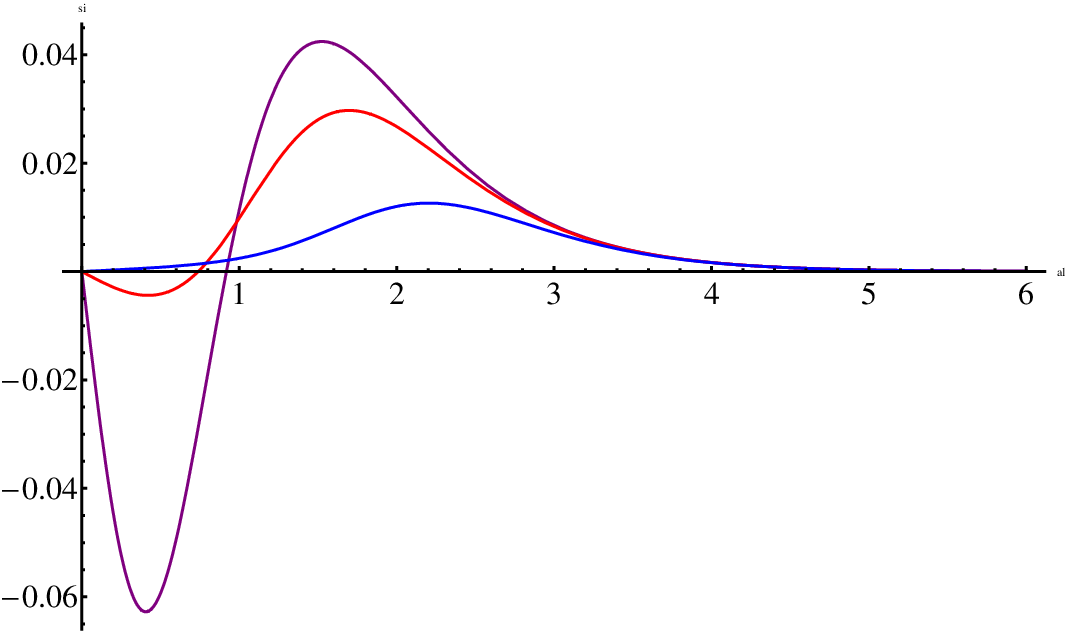
Figure 2: The mode-dependent pumped current Eq. () as a function of ky​Lk_{y}L. The curves correspond to λ=0.01\lambda=0.01 (purple), λ=2\lambda=2 (red), and λ=5\lambda=5 (blue).

Fig. 2 shows ∑σ,σ′=±Πσ​σ′(ky)\sum_{\sigma,\sigma^{\prime}=\pm}\,\Pi_{\sigma\sigma^{\prime}}(k_{y}) [Eq. () in units of 4​λ​U−24\lambda U^{-2} ], which is essentially the mode-dependent pumped current, as a function of kyk_{y}. We see that ∑σ,σ′=±Πσ​σ′(ky=0)=0\sum_{\sigma,\sigma^{\prime}=\pm}\,\Pi_{\sigma\sigma^{\prime}}(k_{y}=0)=0, i.e. waves with transverse momentum ky=0k_{y}=0 that are incident perpendicular to the interface do not contribute to the pumped current, which is a manifestation of the Klein paradox [14, 15]. We also see that negative mode-contributions only occur for small values of λ\lambda. From Eq. () it follows that the largest contribution to ∑σ,σ′=±Πσ​σ′\sum_{\sigma,\sigma^{\prime}=\pm}\,\Pi_{\sigma\sigma^{\prime}} comes from the transverse modes ky​L∼0.1​λk_{y}L\sim 0.1\,\lambda for λ∼50\lambda\sim 50, similarly as for the transmission (conductance) in the same system [17].

Refer to caption
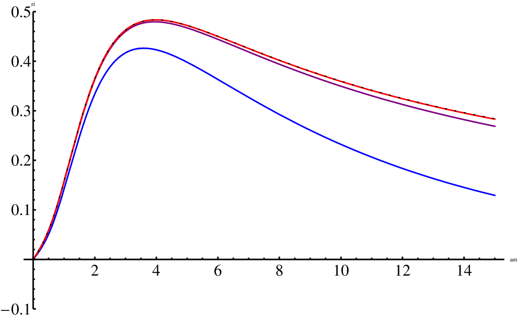
Figure 3: The total pumped current IpI_{p} as a function of λ\lambda, for W/L=100W/L=100. The blue, purple and red lines represent the exact sum over kyk_{y} of the integrand in Eq. () for nn=100, 150 and 200 modes. The black dotted line is the integrated result Eq. (35c).

Fig. 3 shows a plot of the total pumped current IpI_{p} as a function of λ\lambda, for a fixed value of W/L=100W/L=100. For n∼200n\sim 200 modes the sum converges to the continuum result. The number of modes needed for convergence becomes larger for W/LW/L larger, while for W/L=20W/L=20 only n∼20n\sim 20 modes are needed. As expected, Ip​(t⟂=0)=0I_{p}(t_{\perp}=0)=0, since in the absence of interlayer coupling the bilayer reduces to two uncoupled monolayers for which the pumping parameters V1​(t)V_{1}(t) and V2​(t)V_{2}(t) become uncoupled and no pumping occurs. From Eq. (35c) we obtain that for small interlayer coupling strength t⟂≪1/Lt_{\perp}\ll 1/L the pumped current IpI_{p} scales as

limt⟂→0Ip=4​ln⁡2−164​π2​ω​e​WL​sin⁡ϕ​δ​U1​δ​U2U2​λ,\lim_{t_{\perp}\rightarrow 0}I_{p}=\frac{4\ln 2-1}{64\pi^{2}}\,\omega e\,\frac{W}{L}\,\sin\phi\,\frac{\delta U_{1}\delta U_{2}}{U^{2}}\,\lambda, (36)

hence IpI_{p} depends linearly on t⟂t_{\perp} for t⟂=1/l⟂≪1/Lt_{\perp}=1/l_{\perp}\ll 1/L. On the other hand, in the limit of large interlayer coupling t⟂=1/l⟂≫1/Lt_{\perp}=1/l_{\perp}\gg 1/L we find

limt⟂→∞Ip=34​π2​ω​e​WL​sin⁡ϕ​δ​U1​δ​U2U2​ln⁡λλ,\lim_{t_{\perp}\rightarrow\infty}I_{p}=\frac{3}{4\pi^{2}}\,\omega e\,\frac{W}{L}\,\sin\phi\,\frac{\delta U_{1}\delta U_{2}}{U^{2}}\,\frac{\ln\lambda}{\lambda}, (37)

and hence Ip∼ln⁡t⟂​Lt⟂​LI_{p}\sim\frac{\ln t_{\perp}L}{t_{\perp}L} in this limit. In between these two limits IpI_{p} exhibits a maximum which is determined by d​Ip/d​λ=0dI_{p}/d\lambda=0 and yields

λmax=3.88→Ip​(λmax)=0.51​ω​e2​π2​WL​sin⁡ϕ​δ​U1​δ​U2U2.\lambda_{\rm max}=3.88\ \ \rightarrow\ \ I_{p}(\lambda_{\rm max})=0.51\,\frac{\omega e}{2\pi^{2}}\,\frac{W}{L}\,\sin\phi\,\frac{\delta U_{1}\delta U_{2}}{U^{2}}. (38)

Thus IpI_{p} is maximal if t⟂t_{\perp} is of the same order as 1/L1/L. The pumped current thus strongly depends on t⟂t_{\perp} and reduces to zero for t⟂→0t_{\perp}\rightarrow 0. This is in sharp contrast with the behavior of the conductance at the Dirac point in a graphene bilayer, which equals the conductance across two monolayers and is independent of t⟂t_{\perp} [17].

V Conclusion

In summary, we have investigated the adiabatically pumped current through a wide graphene bilayer consisting of a central weakly doped graphene sheet coupled to two heavily doped contact regions. At the Dirac point, the pumped current is carried by evanescent waves in the central region and exhibits a cross-over from linear (for t⟂​L≪1t_{\perp}L\ll 1) to logarithmic (for t⟂​L≫1t_{\perp}L\gg 1)-dependence as a function of increasing interlayer coupling strength t⟂t_{\perp}, with a maximum around t⟂​L∼3.88t_{\perp}L\sim 3.88. This scaling behavior with t⟂t_{\perp} is markedly different from the behavior of the conductance GG in the same system, which is independent of t⟂t_{\perp} and equal to the conductance across two monolayers in parallel. In practice, this different behavior of IpI_{p} and GG as a function of t⟂t_{\perp} and LL could be used to distinguish between the conductance and the pumped current.

We can estimate the magnitude of the pumped current using typical experimental parameters [14, 20] t⟂=(0.4​e​V)/(ℏ​vF)≈0.6 109t_{\perp}=(0.4eV)/(\hbar v_{F})\approx 0.6\,10^{9} m-1, U≈0.1U\approx 0.1 V, δ​U≈10\delta U\approx 10 mV, and ω≈1\omega\approx 1 GHz. In order to be able to measure a substantial pumped current, one thus needs sample sizes L∼4/t⟂∼6L\sim 4/t_{\perp}\sim 6 nm, which is smaller than currently available samples of order μ\mum [22]. However, with steady progress towards smaller sample sizes, sample lengths of order 10-100 nm are expected to become available in the future. We then obtain from Eq. (35c):

Ip,m​a​x∼5⋅10−14​WL​sin⁡(ϕ)​AI_{p,max}\sim 5\cdot 10^{-14}\frac{W}{L}\sin(\phi)\,A (39)

which, for W/L∼100−1000W/L\sim 100-1000 is well within experimental reach. Observation of this current would be a striking demonstration of quantum pumping produced by relativistic quantum mechanics.

Acknowledgements.
This work has been supported by the Netherlands Organisation for Scientific Research (NWO).

Appendix A Calculation of the scattering matrix elements and their derivatives

In this appendix we calculate the reflection and transmission coefficients rσ​σ′α​βr_{\sigma\sigma^{\prime}}^{\alpha\beta} and tσ​σ′α​βt_{\sigma\sigma^{\prime}}^{\alpha\beta} (σ,σ′∈{+,−}\sigma,\sigma^{\prime}\in\{+,-\}; α,β\alpha,\beta ∈\in L,RL,R) from Eq. (14) and their derivatives with respect to U1U_{1} and U2U_{2}. These derivatives are then used to calculate the pumped current (33).

Matching the eigenfunctions (14) at the interfaces x=0x=0 and x=Lx=L results in the 8 equations:

r+⁣±​N+​(X2+​V1−X2+​k+X1+​V2−X1+​k+∗)+r−⁣±​N−​(X2−​V1−X2−​k−X1−​V2−X1−​k−∗)\displaystyle r_{+\pm}N_{+}\left(\begin{array}[]{c}X_{2+}V_{1}\\ -X_{2+}k_{+}\\ X_{1+}V_{2}\\ -X_{1+}k_{+}^{*}\end{array}\right)+r_{-\pm}N_{-}\left(\begin{array}[]{c}X_{2-}V_{1}\\ -X_{2-}k_{-}\\ X_{1-}V_{2}\\ -X_{1-}k_{-}^{*}\end{array}\right)
=(c3±c1±c2±c4±)−N±​(X2±​V1X2±​k±∗X1±​V2X1±​k±)\displaystyle\hskip 28.45274pt=\left(\begin{array}[]{c}c_{3\pm}\\ c_{1\pm}\\ c_{2\pm}\\ c_{4\pm}\end{array}\right)-N_{\pm}\,\left(\begin{array}[]{c}X_{2\pm}V_{1}\\ X_{2\pm}k_{\pm}^{*}\\ X_{1\pm}V_{2}\\ X_{1\pm}k_{\pm}\end{array}\right)
t+⁣±​N+​(X2+​V1X2+​k+∗X1+​V2X1+​k+)+t−⁣±​N−​(X2−​V1X2−​k−∗X1−​V2X1−​k−)\displaystyle t_{+\pm}N_{+}\left(\begin{array}[]{c}X_{2+}V_{1}\\ X_{2+}k_{+}^{*}\\ X_{1+}V_{2}\\ X_{1+}k_{+}\end{array}\right)+t_{-\pm}N_{-}\left(\begin{array}[]{c}X_{2-}V_{1}\\ X_{2-}k_{-}^{*}\\ X_{1-}V_{2}\\ X_{1-}k_{-}\end{array}\right)
=(c3±​z−1(c1±−i​t⟂​L​c2±)​zc2±​z(c4±−i​t⟂​L​c3±)​z−1),\displaystyle\hskip 28.45274pt=\left(\begin{array}[]{c}c_{3\pm}z^{-1}\\ (c_{1\pm}-it_{\perp}Lc_{2\pm})z\\ c_{2\pm}z\\ (c_{4\pm}-it_{\perp}Lc_{3\pm})z^{-1}\end{array}\right),

with z≡exp⁡(ky​L)z\equiv\exp(k_{y}L), Vj=−UjV_{j}=-U_{j} at the Dirac point (j=1,2j=1,2) and Xj±X_{j\pm} and N±N_{\pm} given by Eqns. (11) and (12). Eliminating c1−c4c_{1}-c_{4} from Eqns. (A) and (A) yields after some straightforward but lengthy algebra for the four reflection coefficients:

rσ​σ′L​L=ασ​σ′L​L​cosh⁡(2​ky​L)+βσ​σ′L​L​sinh⁡(2​ky​L)+γσ​σ′L​Lδ​cosh⁡(2​ky​L)+ϵ​sinh⁡(2​ky​L)+ηr_{\sigma\sigma^{\prime}}^{LL}=\frac{\alpha_{\sigma\sigma^{\prime}}^{LL}\cosh(2k_{y}L)+\beta_{\sigma\sigma^{\prime}}^{LL}\sinh(2k_{y}L)+\gamma_{\sigma\sigma^{\prime}}^{LL}}{\delta\cosh(2k_{y}L)+\epsilon\sinh(2k_{y}L)+\eta} (72)

with σ,σ′∈{+,−}\sigma,\sigma^{\prime}\in\{+,-\}. Using k±≡kx±+i​kyk_{\pm}\equiv k_{x\pm}+ik_{y}, the dimensionless coupling length λ≡t⟂​L\lambda\equiv t_{\perp}L, A≡X1+​X2−A\equiv X_{1+}X_{2-} and B≡X1−​X2+B\equiv X_{1-}X_{2+}, the coefficients in Eq. (72) are given by:

α+⁣+L​L\displaystyle\alpha_{++}^{LL} =\displaystyle= 2N+N−[iky(k+A2−k+∗B2)+\displaystyle 2\,N_{+}\,N_{-}\,\left[ik_{y}(k_{+}A^{2}-k_{+}^{*}B^{2})\,+\right.
(kx+2−kx−2+2ky2)AB]\displaystyle\left.(k_{x+}^{2}-k_{x-}^{2}+2k_{y}^{2})\,AB\right]
β+⁣+L​L\displaystyle\beta_{++}^{LL} =\displaystyle= 2​N+​N−​kx−​[k+​A2−k+∗​B2−2​i​ky​A​B]\displaystyle 2\,N_{+}\,N_{-}k_{x-}\,\left[k_{+}A^{2}-k_{+}^{*}B^{2}-2ik_{y}AB\right]
γ+⁣+L​L\displaystyle\gamma_{++}^{LL} =\displaystyle= N+N−[λ2(A−B)2V1V2−\displaystyle N_{+}\,N_{-}\,\left[\lambda^{2}(A-B)^{2}V_{1}V_{2}\,-\,\right.
2iλ(A−B)kx−(X1+X1−V2−X2+X2−V1)]−α+⁣+L​L\displaystyle\hskip-7.22743pt\left.2i\lambda(A\hskip-1.4457pt-\hskip-1.4457ptB)k_{x-}(X_{1+}X_{1-}V_{2}\hskip-1.4457pt-\hskip-1.4457ptX_{2+}X_{2-}V_{1})\right]-\alpha_{++}^{LL}
α+⁣−L​L\displaystyle\alpha_{+-}^{LL} =\displaystyle= 2N−2kx−X1−X2−[(kx+−kx−+2iky)A\displaystyle 2\,N_{-}^{2}\,k_{x-}X_{1-}X_{2-}\left[(k_{x+}-k_{x-}+2ik_{y})A\right. (73)
+(kx+−kx−−2iky)B]\displaystyle\left.+\,(k_{x+}-k_{x-}-2ik_{y})B\right]
β+⁣−L​L\displaystyle\beta_{+-}^{LL} =\displaystyle= 2​N−2​kx−​X1−​X2−​(kx++kx−)​(A−B)\displaystyle 2\,N_{-}^{2}k_{x-}X_{1-}X_{2-}(k_{x+}+k_{x-})(A-B)
γ+⁣−L​L\displaystyle\gamma_{+-}^{LL} =\displaystyle= −2​i​λ​N−2​(A−B)​kx−​(X1−2​V2−X2−2​V1)−\displaystyle-2i\lambda\,N_{-}^{2}\,(A-B)\,k_{x-}(X_{1-}^{2}V_{2}-X_{2-}^{2}V_{1})-
α+⁣−L​L\displaystyle\alpha_{+-}^{LL}

and

α−⁣+L​L\displaystyle\alpha_{-+}^{LL} =\displaystyle= α+⁣−L​L​(subindex +↔subindex -)\displaystyle\alpha_{+-}^{LL}(\mbox{\rm\small subindex +}\leftrightarrow\mbox{\rm\small subindex -})
β−⁣+L​L\displaystyle\beta_{-+}^{LL} =\displaystyle= β+⁣−L​L​(subindex +↔subindex -)\displaystyle\beta_{+-}^{LL}(\mbox{\rm\small subindex +}\leftrightarrow\mbox{\rm\small subindex -})
γ−⁣+L​L\displaystyle\gamma_{-+}^{LL} =\displaystyle= γ+⁣−L​L​(subindex +↔subindex -)\displaystyle\gamma_{+-}^{LL}(\mbox{\rm\small subindex +}\leftrightarrow\mbox{\rm\small subindex -})
α−⁣−L​L\displaystyle\alpha_{--}^{LL} =\displaystyle= α+⁣+L​L​(subindex +↔subindex -)\displaystyle\alpha_{++}^{LL}(\mbox{\rm\small subindex +}\leftrightarrow\mbox{\rm\small subindex -})
β−⁣−L​L\displaystyle\beta_{--}^{LL} =\displaystyle= β+⁣+L​L​(subindex +↔subindex -)\displaystyle\beta_{++}^{LL}(\mbox{\rm\small subindex +}\leftrightarrow\mbox{\rm\small subindex -})
γ−⁣−L​L\displaystyle\gamma_{--}^{LL} =\displaystyle= γ+⁣+L​L​(subindex +↔subindex -),\displaystyle\gamma_{++}^{LL}(\mbox{\rm\small subindex +}\leftrightarrow\mbox{\rm\small subindex -}),

Also

δ\displaystyle\delta =\displaystyle= 2N+N−[−(kx+kx−−ky2)(A2+B2)\displaystyle 2\,N_{+}\,N_{-}\,\left[-(k_{x+}k_{x-}-k_{y}^{2})(A^{2}+B^{2})\right. (75a)
+(kx+2+kx−2−2ky2)AB]\displaystyle\left.+\,(k_{x+}^{2}+k_{x-}^{2}-2k_{y}^{2})AB\right]
ϵ\displaystyle\epsilon =\displaystyle= 2iN+N−[−(kx++kx−)ky(A2+B2)\displaystyle 2i\,N_{+}\,N_{-}\,\left[-(k_{x+}+k_{x-})k_{y}\,(A^{2}+B^{2})\right. (75b)
+ 2(kx++kx−)kyAB]\displaystyle\left.+\,2\,(k_{x+}+k_{x-})k_{y}\,AB\right]
η\displaystyle\eta =\displaystyle= N+N−[−λ2(A−B)2V1V2\displaystyle N_{+}\,N_{-}\,\left[-\lambda^{2}(A-B)^{2}V_{1}V_{2}\right. (75c)
−2​i​λ​(kx+−kx−)​(A−B)​(X1+​X1−​V2−X2+​X2−​V1)\displaystyle-2i\lambda(k_{x+}-k_{x-})(A-B)(X_{1+}X_{1-}V_{2}-X_{2+}X_{2-}V_{1})
−2(kx+kx−+ky2)(A−B)2−2(kx+−kx−)2AB]\displaystyle\left.-2(k_{x+}k_{x-}\hskip-1.4457pt+\hskip-1.4457ptk_{y}^{2})(A\hskip-1.4457pt-\hskip-1.4457ptB)^{2}\hskip-1.4457pt-\hskip-1.4457pt2(k_{x+}\hskip-1.4457pt-\hskip-1.4457ptk_{x-})^{2}AB\right]

The transmission coefficients in Eq. (A) are given by

t+⁣+R​L\displaystyle t_{++}^{RL} =\displaystyle= μ+⁣+R​L​cosh⁡(ky​L)−ν+⁣+R​L​sinh⁡(ky​L)δ​cosh⁡(2​ky​L)+ϵ​sinh⁡(2​ky​L)+η\displaystyle\frac{\mu_{++}^{RL}\cosh(k_{y}L)-\nu_{++}^{RL}\sinh(k_{y}L)}{\delta\cosh(2k_{y}L)+\epsilon\sinh(2k_{y}L)+\eta} (76a)
t+⁣−R​L\displaystyle t_{+-}^{RL} =\displaystyle= μ+⁣−R​L​cosh⁡(ky​L)−ν+⁣−R​L​sinh⁡(ky​L)δ​cosh⁡(2​ky​L)+ϵ​sinh⁡(2​ky​L)+η\displaystyle\frac{\mu_{+-}^{RL}\cosh(k_{y}L)-\nu_{+-}^{RL}\sinh(k_{y}L)}{\delta\cosh(2k_{y}L)+\epsilon\sinh(2k_{y}L)+\eta} (76b)
t−⁣+R​L\displaystyle t_{-+}^{RL} =\displaystyle= t+⁣−R​L​(subindex +↔subindex -)\displaystyle t_{+-}^{RL}(\mbox{\rm\small subindex +}\leftrightarrow\mbox{\rm\small subindex -}) (76c)
t−⁣−R​L\displaystyle t_{--}^{RL} =\displaystyle= t+⁣+R​L​(subindex +↔subindex -).\displaystyle t_{++}^{RL}(\mbox{\rm\small subindex +}\leftrightarrow\mbox{\rm\small subindex -}). (76d)

with

μ+⁣+R​L\displaystyle\mu_{++}^{RL} =\displaystyle= −2N+N−(A−B)kx+[2kx−(A−B)\displaystyle-2\,N_{+}\,N_{-}\,(A-B)\,k_{x+}\,\left[2k_{x-}(A-B)\right.
+iλ(X1+X1−V2−X2+X2−V1)]\displaystyle\left.+\,i\lambda(X_{1+}X_{1-}V_{2}-X_{2+}X_{2-}V_{1})\right]
ν+⁣+R​L\displaystyle\nu_{++}^{RL} =\displaystyle= 4​i​N+​N−​(A−B)2​kx+​ky\displaystyle 4i\,N_{+}\,N_{-}\,(A-B)^{2}\,k_{x+}k_{y}
μ+⁣−R​L\displaystyle\mu_{+-}^{RL} =\displaystyle= −2​i​λ​N−2​(A−B)​kx−​(X1−2​V2−X2−2​V1)\displaystyle-2i\,\lambda\,N_{-}^{2}\,(A-B)\,k_{x-}(X_{1-}^{2}V_{2}-X_{2-}^{2}V_{1})
ν+⁣−R​L\displaystyle\nu_{+-}^{RL} =\displaystyle= 2N−2(A−B)kx−[iλ(X1−2V2+X2−2V1)\displaystyle 2\,N_{-}^{2}\,(A-B)\,k_{x-}\left[i\lambda(X_{1-}^{2}V_{2}+X_{2-}^{2}V_{1})\right. (77)
−2X1−X2−(kx+−kx−)]\displaystyle\left.-2\,X_{1-}X_{2-}(k_{x+}-k_{x-})\right]

In two limiting cases the reflection- and transmission coefficients (72) and (76) reduce to simple forms

:
1) For L→0L\rightarrow 0, the ++- and −--modes decouple and we obtain from Eq. (76)

t+⁣+R​L→1andt+⁣−R​L→0.t_{++}^{RL}\rightarrow 1\ \ \mbox{\rm and}\ \ t_{+-}^{RL}\rightarrow 0. (78)

2) For t⟂→0t_{\perp}\rightarrow 0, i.e. in the absence of interlayer coupling, the reflection- and transmission coefficients (72) and (76) reduce to the monolayer expressions [15, 16]

r+⁣+L​L\displaystyle r_{++}^{LL} →t⟂→0\displaystyle\stackrel{{\scriptstyle t_{\perp}\rightarrow 0}}{{\rightarrow}} (kx+−i​ky)​sinh⁡(ky​L)kx+​cosh⁡(ky​L)+i​ky​sinh⁡(ky​L)\displaystyle\frac{(k_{x+}-ik_{y})\sinh(k_{y}L)}{k_{x+}\cosh(k_{y}L)+ik_{y}\sinh(k_{y}L)} (79a)
→|V1|,|V2|→∞\displaystyle\stackrel{{\scriptstyle|V_{1}|,|V_{2}|\rightarrow\infty}}{{\rightarrow}} tanh⁡(ky​L)\displaystyle\tanh(k_{y}L)
t+⁣+R​L\displaystyle t_{++}^{RL} →t⟂→0\displaystyle\stackrel{{\scriptstyle t_{\perp}\rightarrow 0}}{{\rightarrow}} kx+kx+​cosh⁡(ky​L)+i​ky​sinh⁡(ky​L)\displaystyle\frac{k_{x+}}{k_{x+}\cosh(k_{y}L)+ik_{y}\sinh(k_{y}L)} (79b)
→|V1|,|V2|→∞\displaystyle\stackrel{{\scriptstyle|V_{1}|,|V_{2}|\rightarrow\infty}}{{\rightarrow}} 1cosh⁡(ky​L)\displaystyle\frac{1}{\cosh(k_{y}L)}
t+⁣−R​L\displaystyle t_{+-}^{RL} →t⟂→0\displaystyle\stackrel{{\scriptstyle t_{\perp}\rightarrow 0}}{{\rightarrow}} 0.\displaystyle 0. (79c)

The reflection- and transmission coefficients for right-incident Dirac fermions rσ​σ′R​Rr_{\sigma\sigma^{\prime}}^{RR} and tσ​σ′L​Rt_{\sigma\sigma^{\prime}}^{LR} (σ,σ′∈{+,−}\sigma,\sigma^{\prime}\in\{+,-\}) are given by Eqns. (72) and (76) by interchanging the layer subindices 1 and 2. So r+⁣+R​R=r+⁣+L​Lr_{++}^{RR}=r_{++}^{LL} (subindex 1 ↔\leftrightarrow subindex 2) etc.

In order to calculate the pumped current (33), we need the derivatives of rσ​σ′L​Lr_{\sigma\sigma^{\prime}}^{LL} and tσ​σ′L​Rt_{\sigma\sigma^{\prime}}^{LR} with respect to U1U_{1} and U2U_{2}. These can be calculated by splitting the coefficients α+⁣+L​L\alpha_{++}^{LL} etc. in Eq. (72) into real and imaginary parts and differentiating each of these with respect to V1V_{1} and V2V_{2}. The latter does not make any difference for the current, since only products of derivatives with respect to U1U_{1} and U2U_{2} enter Eq. (33) which are the same as those of the corresponding derivatives with respect to V1V_{1} and V2V_{2} (since Vj=−UjV_{j}=-U_{j} for ϵ=0\epsilon=0, j=1,2j=1,2). The resulting expressions for the derivatives are rather lengthy and therefore not given here. For equal bias voltages V1=V2≡VV_{1}=V_{2}\equiv V (as required for a true pumping process) and in the limit of V→∞V\rightarrow\infty, however, an analytic expression for the pumped current IpI_{p} [Eq. (2) can be derived. This expression is obtained by first taking the limit V1→V2V_{1}\rightarrow V_{2}, for which X1−→X2−=2​t⟂​VX_{1-}\rightarrow X_{2-}=2t_{\perp}V and X1+→−X2+=(V1−V2)​(V+t2)→0X_{1+}\rightarrow-X_{2+}=(V_{1}-V_{2})(V+\frac{t}{2})\rightarrow 0 (see Eq. (11)). We then expand all terms in the Eq. (34) in orders of V1−V2V_{1}-V_{2} (or, equivalently, X1+X_{1+}) and find that while the numerators contain terms of order (V1−V2)7(V_{1}-V_{2})^{7} and higher, all terms in the denominator are proportional to (V1−V2)8(V_{1}-V_{2})^{8}. In the limit of V→∞V\rightarrow\infty, assuming V≫t⟂,kyV\gg t_{\perp},k_{y} and V​t⟂≫ky2Vt_{\perp}\gg k_{y}^{2}, the terms of order (V1−V2)7(V_{1}-V_{2})^{7} in the numerator cancel and we are left with a finite pumped current which to highest order in VV amounts to:

∑σ,σ′=±\displaystyle\sum_{\sigma,\sigma^{\prime}=\pm} Πσ​σ′(ky)=4​λU2×\displaystyle\!\!\Pi_{\sigma\sigma^{\prime}}(k_{y})=\frac{4\lambda}{U^{2}}\times
(λ2+6​ky​L​sinh⁡(2​ky​L)−8​cosh2⁡(ky​L))​sinh⁡(2​ky​L)(λ2+4​cosh2⁡(ky​L))3\displaystyle\hskip-14.45377pt\frac{\left(\lambda^{2}\hskip-1.4457pt+\hskip-1.4457pt6k_{y}L\sinh(2k_{y}L)\hskip-1.4457pt-\hskip-1.4457pt8\cosh^{2}(k_{y}L)\right)\sinh(2k_{y}L)}{\left(\lambda^{2}+4\cosh^{2}(k_{y}L)\right)^{3}}

Integration of () over the transverse modes kyk_{y} then leads to the pumped current Eq. (35) in the main text.

References

  • [1] B.L. Altshuler and L.I. Glazman, Science 283, 1864 (1999).
  • [2] D.J. Thouless, Phys. Rev. B 27, 6083 (1983).
  • [3] P.W. Brouwer, Phys. Rev. B 58, R10135 (1998).
  • [4] M. Büttiker, H. Thomas, and A. Prêtre, Z. Phys. B 94, 133 (1994).
  • [5] B. Spivak, F. Zhou and M. T. BealMonod, Phys. Rev. B 51, 13226 (1995).
  • [6] J. E. Avron, A. Elgart, G. M. Graf, and L. Sadun, Phys. Rev. B 62, R10618 (2000).
  • [7] J. Wang, Y. Wei, B. Wang and H. Guo, Appl. Phys. Lett. 79, 3977 (2001); M. Blaauboer, Phys. Rev. B 65, 235318 (2002); F. Taddei, M. Governale and R. Fazio, Phys. Rev. B 70, 052510 (2004).
  • [8] See e.g. J. Splettstoesser, M. Governale, J. König, R. Fazio, Phys. Rev. Lett. 95, 246803 (2005); E. Sela and Y. Oreg, Phys. Rev. Lett. 96, 166802 (2006).
  • [9] E.R. Mucciolo, C. Chamon and C.M. Marcus, Phys. Rev. Lett. 89, 146802 (2002); P. Sharma and P.W. Brouwer, Phys. Rev. Lett. 91, 166801 (2003). S.K. Watson, R.M. Potok, C.M. Marcus and V. Umansky, Phys. Rev. Lett. 91, 258301 (2003).
  • [10] Y. Wei, J. Wang, H. Guo, and C. Roland, Phys. Rev. B 64, 115321 (2001); M.R. Buitelaar et al., Phys. Rev. Lett. 101, 126803 (2008); V. Zólyomi, L. Oroszlány, and C.J. Lambert, Phys. Status Solidi 246, 2650 (2009).
  • [11] E. Prada, P. San-Jose, and H. Schomerus, Phys. Rev. B 80, 245414 (2009); ibid. ArXiv:1007.3161v1 [cond-mat.mtrl-sci]
  • [12] R. Zhu and H. Chen, Appl. Phys. Lett. 95, 122111 (2009).
  • [13] K.S. Novoselov, A.K. Geim, S.V. Morozov, D. Jiang, Y. Zhang, S.V. Dubonos, I.V. Grigorieva, and A.A. Firsov, Science 306, 666 (2004).
  • [14] A.H. Castro Neto, F. Guinea, N.M.R. Peres, K.S. Novoselov, and A.K. Geim, Rev. Mod. Phys. 81, 109 (2009).
  • [15] M.I. Katsnelson, Eur. Phys. J. B 51, 157 (2006).
  • [16] J. Tworzydło, B. Trauzettel, M. Titov, A. Rycerz and C.W.J. Beenakker, Phys. Rev. Lett. 96, 246802 (2006).
  • [17] I. Snyman and C.W.J. Beenakker, Phys. Rev. B 75, 045322 (2007).
  • [18] Hamiltonians in which also different couplings were taken into account can be found in Ref. [14].
  • [19] Our pumped current can also be considered as a rectified net dc current between the left and right leads that is induced by an ac voltage bias between the top and bottom leads in the geometry of Fig. 1.
  • [20] E.V. Castro, K.S. Novoselov, S.V. Morozov, N.M.R. Peres, J.M.B. Lopes dos Santos, J. Nilsson, F. Guinea, A.K. Geim, and A.H. Castro Neto, J. Phys.: Condens. Matter 22, 175503 (2010).
  • [21] M.I. Katsnelson, K.S. Novoselov and A.K. Geim, Nature Physics 2, 620 (2006).
  • [22] M.F. Craciun, S. Russo, M. Yamamoto, J.B. Oostinga, A.F. Morpurgo, and S. Tarucha, Nature Nanotechnology 4, 383 (2009); B.E. Feldman, J. Martin and A. Yacoby, Nature Physics 5, 889 (2009).