Field Reconstruction in Sensor Networks
with Coverage Holes and Packet Losses

Let us consider an $n\times n$ non-negative definite random matrix ${\bf A}$, whose eigenvalues are denoted by $\lambda_{{\bf A},1},\ldots,\lambda_{{\bf A},n}$.

Next, consider the matrix ${\bf V}$ as defined in (3) and that the LMMSE filter is used for field reconstruction. Then, the estimate of the unknown vector ${\bf a}$ in (4), given ${\bf y}$ and ${\bf V}$, is obtained by computing $\hat{{\bf a}}=\mathbb{E}[{\bf a}{\bf p}\mathsf{{}^{H}}]\mathbb{E}[{\bf p}{\bf p}\mathsf{{}^{H}}]^{-1}{\bf p}$. Through easy computations and using the Sherman-Morrison-Woodbury identity, we can obtain the MSE as

where $\gamma=\sigma^{2}_{a}/\sigma^{2}_{n}$ denotes the signal-to-noise ratio on the sensor measurements, and we employed the definition of the $\eta$-transform given in (5).

Next, we approximate the MSE of the finite size system in (4) through an asymptotic model, which assumes the size of ${\bf V}$ to grow to infinity while the ratio of its number of rows to its number of columns tends to a finite limit, $\beta$, greater than zero, i.e., we assume

Indeed, in our recent works [8, 9, 10] it was shown that this asymptotic model provides a tight approximation of the MSE of the finite size system, already for small values of $n$ and $m$. Under these conditions, we therefore define the asymptotic expression of the MSE as [10]:

if the limit exists.

Vandermonde matrices have been studied in a number of recent works [8, 9, 10, 11]. Specifically, [9] considered the case where the vectors ${\bf x}_{q}$ are i.i.d., for $q=1,\ldots,m$, and their entries, $x_{qj}$ are i.i.d. random variables with uniform distribution in $[-1/2,1/2)$. The work there studied the eigenvalue distribution of ${\bf V}{\bf V}\mathsf{{}^{H}}$ for both finite and infinite (i.e., $m,n\rightarrow\infty$) matrix size. Although an explicit expression of such LSD is still unknown, [9] provided an algorithm to compute its moments of any order in closed form.

Indeed, as $n,m\rightarrow\infty$ with $\beta_{n,m}=n^{d}/m$ having a finite limit $\beta>0$, in [9] it was shown that the $p$-th moment of the generic asymptotic eigenvalue of ${\bf V}{\bf V}\mathsf{{}^{H}}$, denoted by $\lambda$, is given by

where $f_{\lambda,u}(d,\beta,z)$ represents the distribution of $\lambda$. Moreover, $\Omega_{p,k}$ is the set of partitions of the set ${\cal P}=\{1,2,\ldots,p\}$ in $k$ subsets, and $v(\boldsymbol{\omega})\in(0,1]$, $\boldsymbol{\omega}\in\Omega_{p,k}$ is a rational number that can be analytically computed from $\boldsymbol{\omega}$ following the procedure described in [9]. The subscript $u$ in $M_{p,d,\beta,u}$ and $f_{\lambda,u}(d,\beta,z)$ indicates that a uniform distribution of the entries of ${\bf x}_{q}$ is considered in the matrix ${\bf V}$.

In [9] it was also shown that when $n,m,d\rightarrow\infty$, with $\beta_{n,m}=n^{d}/m$ having a finite limit $\beta>0$, the eigenvalue distribution $f_{\lambda,u}(d,\beta,z)$ converges to the Marčcenko-Pastur law [24]. A similar result [10] also applies when the vectors ${\bf x}_{q}$ ($q=1,\ldots,m$) are independent but not i.i.d., with equally spaced averages.

More recently, Ryan and Debbah in [11] considered $d=1$ and the case where the random variables $x_{q1}$, $q=1,\ldots,m$, are i.i.d. with continuous distribution $f_{x}(z)$, $0\leq z<1$. Under such hypothesis, it was shown that the asymptotic moments of ${\bf V}{\bf V}\mathsf{{}^{H}}$ can be written as

where the terms $I_{k}$ depend on the phase distribution $f_{x}(z)$ and are given by

for $k\geq 1$. The subscript $x$ in $M_{p,1,\beta,x}$ indicates that in the matrix ${\bf V}$ the random variables $x_{q1}$ have a generic continuous distribution $f_{x}(z)$. Note that for the uniform distribution we have $I_{k}=1$, for all $k$. The important result in (8) states that, given $\beta$, if the moments of ${\bf V}{\bf V}\mathsf{{}^{H}}$ are known for uniformly distributed phases, they can be readily obtained for any continuous phase distribution $f_{x}(z)$.

We consider a wireless sensor network whose nodes are uniformly distributed over a geographical region. Without loss of generality, we assume a square region of unitary side ($d=2$, ${\cal H}=[-1/2,+1/2]^{2}$), where the sink is located at the center and has coordinates $(z_{1},z_{2})=(0,0)$. Through direct transmissions, the sensors periodically send messages to the sink, including their measurements. At every sample period, a sensor message is correctly received at the sink if its signal-to-noise ratio (SNR) exceeds a threshold $\tau$. The communication channel is assumed to be affected by slow fading and to be stationary over the message duration.

Let $d$ be the distance between a generic sensor and the sink. Then, the signal to noise ratio at the receiver is given by

where $h\sim{\cal N}_{\mathbb{C}}(0,1)$ is a circularly symmetric Gaussian complex random variable representing the channel gain, and $s$ is the signal to noise ratio in the absence of fading and when the sensor-sink distance is $d=1$.

The probability that a message is correctly received at the sink is given by

with $a=\tau/s$ and $F_{|h|^{2}}(z)=1-{\rm e}^{-z}$ being the cumulative density function of $|h|^{2}$.

The probability density $f_{x}(z_{1},z_{2})$ corresponding to sensors at distance $d=\sqrt{z_{1}^{2}+z_{2}^{2}}$, $-1/2\leq z_{1},z_{2}\leq 1/2$ from the sink and successfully sending a message is then given by

where $f_{u}(z_{1},z_{2})=1\,\forall z_{1},z_{2}$, is the density representing the sensor deployment (recall that nodes are assumed to be uniformly distributed in the region hence their density is constant and equal to 1). Using (18), we obtain:

where

In order to compute (14), we need the function $g_{x}(y)$, i.e., the density of $f_{x}(z_{1},z_{2})$. Note that $f_{x}(z_{1},z_{2})$ is circularly symmetric with respect to $(z_{1},z_{2})=(0,0)$. Let $y$ be the value of density of the sampling points at distance $d_{y}=\sqrt{z_{1}^{2}+z_{2}^{2}}$ from the sink. Then, from (19) we obtain $d_{y}=\sqrt{\frac{1}{a}\log\frac{b}{y}}$, thus the network area where the density is lower than $y$ is given by

for $0\leq d_{y}\leq 1/2$, i.e., $b{\rm e}^{-a/4}\leq y<b$. For $1/2<d_{y}<\sqrt{2}/2$, it is possible to show that

In conclusion,

and

Since $|{\cal A}|=1$, then the asymptotic MSE can be obtained by computing

Figure 2 shows the density $g_{x}(y)$ for $a=0,5,10$ dB. Note that $a=\tau/s$, thus for a fixed $s$ (i.e., the signal to noise ratio at distance $D$ in the absence of fading) the parameter $a$ is proportional to the SNR threshold $\tau$. In particular, as $\tau$ decreases, the probability that a message successfully reaches the destination increases and, thus, the spatial distribution of correctly received samples, $f_{x}(z_{1},z_{2})$, tends to the uniform distribution $f_{u}(z_{1},z_{2})$. As a consequence, the density of $f_{x}(z_{1},z_{2})$, i.e., $g_{x}(y)$, for $a=0$ and 5 dB is concentrated close to $y=1$. However, for high values of $\tau$, messages originated from sensor nodes located far from the sink are successfully received with low probability. Thus, $g_{x}(y)$ shows a significant probability mass around $y=0$.

Figure 3 shows the effect of the fading channel on the MSE of the reconstructed field (dashed lines), and compares the obtained results with the MSE obtained in absence of fading (solid lines). The plot considers different values of $\beta$, namely, $\beta=0.2,0.4,0.6,0.8$, and $a=5$ dB. The MSE is plotted versus the signal to noise ratio on the sensor measurements, $\gamma$. The curves have been obtained by numerically computing (22), where $g_{x}(y)$ is given by (21) and $\eta_{u}(2,\beta,\gamma/\beta)$ is replaced by $\eta^{(n)}_{u}(2,\beta_{n,m},\gamma/\beta_{n,m})$, with $n=10$. Recall that the analytic expression of the LSD $f_{\lambda,u}(d,\beta,z)$ is unknown, hence in the numerical results we considered the AESD $f^{(n)}_{\lambda,u}(d,\beta_{n,m},z)$ instead. We observe that for low values $\beta$, in spite of the presence of fading, the sink node still receives a large number of samples from the sensors, hence the degradation of the MSE shown in Figure 3 is negligible. On the contrary, for $\beta>0.4$ (i.e., for a larger value of the ratio of the number of harmonics composing the approximated field to the number of sensors), the reconstruction performance degrades significantly and this is particularly evident in presence of high values of $\gamma$.

In the case of massively dense networks, the LSD of ${\bf V}{\bf V}\mathsf{{}^{H}}$ is given by (16) and from (17) we know that the MSE tends to 0 as $\beta\rightarrow\infty$. This result is confirmed by the plot in Figure 4, which shows the AESD $f^{(n)}_{\lambda,x}(2,\beta_{n,m},z)$, for $|{\cal A}|=1$, $a=5$ dB, and $n=10$. The behavior of such a function is compared with the density $g_{x}(z)$ as $\beta$ varies. We note that, as $\beta$ decreases, the matching between $f^{(n)}_{\lambda,x}(2,\beta_{n,m},z)$ and $g_{x}(z)$ improves, and the latter represents an excellent approximation already for $\beta=0.01$, as predicted by the result in (V.3).

In environmental monitoring applications, it is often desirable to vary the resolution level with which the field measurements are taken over the region under observation, depending on the field variations and the interest level of the different locations [2, 3]. It follows that the number of samples generated by the sensors network (i.e., the offered traffic load) varies in the spatial domain.

To represent such a scenario, we consider a wireless sensor network whose nodes are uniformly deployed over a square region. We also identify $L$ areas, $A_{i}$ $i=1,\ldots,L$, each corresponding to a different value of the offered traffic load. As often assumed in the literature (see e.g., [26, 27]) and widely applied in the practice, the network is divided into clusters and a hierarchy of clusters is created. More specifically, at the first hierarchical layer, layer 1, the sensors are grouped into clusters, each of which is controlled by a cluster-head. The cluster-head is in charge of handling all traffic packets it receives from the nodes. At a given layer $h>1$ of the hierarchy, the cluster-heads are grouped into clusters on their turn and forward the traffic to their parent cluster-head. At the highest layer, layer $H$, we have only one cluster whose cluster-head coincides with the sink node. Without loss of generality, we assume that the cluster at the $H$-th layer is composed of $L$ cluster-heads, each handling the traffic generated within one of the $L$ areas defined above.

As for the medium access control (MAC) layer, we consider that the nodes implement the IEEE 802.15.4 standard specifications for wireless sensor networks [15]. In particular, all nodes within a cluster are in radio visibility of each other and use the slotted carrier-sense multiple-access/collision avoidance (CSMA/CA) technique [15]. This is a contention-based scheme and transmissions may fail if two or more sensors access the channel at the same time. Inter-cluster interference is instead avoided by assigning different frequency channels to neighboring clusters. We consider that packets, whose transmission fails, are discarded.

In order to derive the probability that a packet transmission fails within a cluster due to collision, we use the Markov chain model presented in [28]. We denote by $m_{i,h}$ the average number of sensors belonging to the generic cluster at the $h$-th layer of the hierarchical architecture, in area $A_{i}$ ($i=1,\ldots,L$ and $h=1,\ldots,H$). Similarly, we define $\lambda_{i,h}$ as the average traffic load per node, again within the generic cluster at the $h$-th layer, in area $A_{i}$. Then, we set the size of the packet payload to 32 bytes, and the value of the other parameters as in [28]. Under this setting, we compute the value of the collision probability within the generic cluster at layer $h$, in area $A_{i}$, as a function of $m_{i,h}$ and $\lambda_{i,h}$, i.e., $P_{c}(i,h)$ [28]. Furthermore, we observe that at the generic layer $h$, with $1<h\leq H$, a node, which acts as cluster-head at layer $h-1$ in area $A_{i}$, will have a traffic load equal to $\lambda_{i,h}=m_{i,h-1}\lambda_{i,h-1}\left[1-P_{c}(i,h-1)\right]$.

It follows that the probability that a packet is successfully delivered to the corresponding $h$-layer cluster-head within area $A_{i}$ ($i=1,\ldots,L$) can be obtained as $P_{s}(i,h)=1-P_{c}(i,h)$. Then, the probability that a measurement generated by a sensor located in $A_{i}$ ($i=1,\ldots,L$) is successfully delivered to the sink is given by:

Next, denoting by $|A_{i}|$ the measure of $A_{i}$, we define

as the normalized probability that a message is successfully delivered to the sink. Then, the spatial density of the sensors successfully sending their message is as follows:

The density of $f_{x}(z_{1},z_{2})$ is therefore given by

and the asymptotic MSE is given by

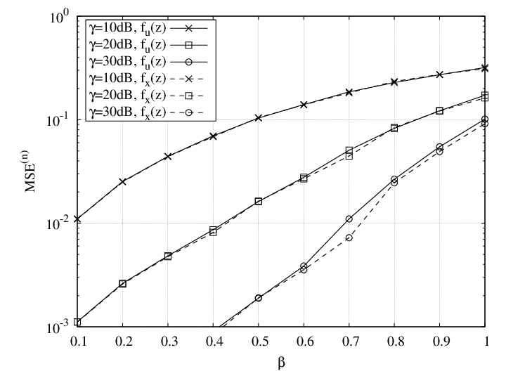
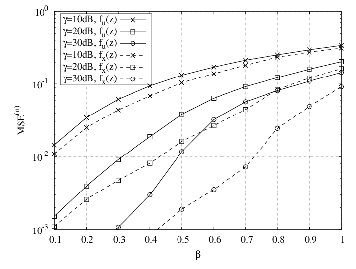
Figures 5 and 6 show the impact of collisions due to the contention-based channel access, on the quality of the reconstructed field. In particular, they compare the MSE of the reconstructed field when collisions are taken into account ($f_{x}({\bf z})$) with the one obtained in the idealistic case where all messages (measurements) sent by the sensors successfully reach the sink ($f_{u}({\bf z})$). The results refer to a square region of unitary side, where there are four areas of equal size ($|A_{i}|=1/4$, $i=1,\ldots,4$) but corresponding to different resolution levels in the measurements collection (i.e., they are characterized by different traffic loads); the number of hierarchical levels is set to $H=3$. We set $\lambda_{1,1}=10^{-3}$, $\lambda_{2,1}=2\cdot 10^{-4}$, $\lambda_{3,1}=2\cdot 10^{-4}$, $\lambda_{4,1}=2\cdot 10^{-5}$ in Figure 5, and a higher traffic load in Figure 6, i.e., $\lambda_{1,1}=5\cdot 10^{-3}$, $\lambda_{2,1}=10^{-3}$, $\lambda_{3,1}=10^{-3}$, $\lambda_{4,1}=10^{-4}$.

Looking at the plots, we observe that both $\beta$ and $\gamma$ have a significant impact of the obtained MSE, with the MSE increasing as $\beta$ grows and smaller values of $\gamma$ are considered. Most interestingly, by comparing the two figures, we can see that as the traffic load, hence the collision probability, increases, the performance derived taking into account the contention-based channel access significantly differs from the idealistic one. Furthermore, the latter effect is particularly evident as $\gamma$ increases, since the higher the signal-to-noise ratio, the more valuable the samples sent by the sensors toward the sink.

References

- [1] D. E. Culler and H. Mulder, Smart sensors to network the world, Scientific American, June 2004.
- [2] M. Perillo, Z. Ignjatovic, and W. Heinzelman, “An energy conservation method for wireless sensor networks employing a blue noise spatial sampling technique,” International Symposium on Information Processing in Sensor Networks (IPSN 2004), Apr. 2004.
- [3] R. Willett, A. Martin, and R. Nowak, “Backcasting: adaptive sampling for sensor networks,” International Symposium on Information Processing in Sensor Networks (IPSN 2004), Apr. 2004.
- [4] F. A. Marvasti, Nonuniform sampling: Theory and practice, Kluwer Academic: Plenum, New York, 2001.
- [5] D. Ganesan, S. Ratnasamy, H. Wang, and D. Estrin, “Coping with irregular spatio-temporal sampling in sensor networks,” ACM SIGCOMM, pp. 125–130, Jan. 2004.
- [6] P. Zhao, C. Zhao, and P. G. Casazza, “Perturbation of regular sampling in shift-invariant spaces for frames,” IEEE Transactions on Information Theory, Vol. 52, No. 10, pp. 4643–4648, Oct. 2006.
- [7] D. S. Early and D. G. Long, “Image reconstruction and enhanced resolution imaging from irregular samples,” IEEE Transactions on Geoscience and Remote Sensing, Vol. 39, No. 2, pp. 291–302, Feb. 2001.
- [8] A. Nordio, C.-F. Chiasserini, and E. Viterbo, “Performance of linear field reconstruction techniques with noise and uncertain sensor locations,” IEEE Transactions on Signal Processing, Vol. 56, No. 8, pp. 3535–3547, Aug. 2008.
- [9] A. Nordio, C.-F. Chiasserini, and E. Viterbo, “Reconstruction of multidimensional signals from irregular noisy samples,” IEEE Transactions on Signal Processing, Vol. 56, No. 9, pp. 4274–4285, Sept. 2008.
- [10] A. Nordio, C.-F. Chiasserini, and E. Viterbo, “Asymptotic analysis of multidimensional jittered sampling,” IEEE Transactions on Signal Processing, Vol. 58, No. 1, pp. 258–268, Jan. 2010.
- [11] Ø. Ryan, and M. Debbah, “Asymptotic behavior of random Vandermonde matrices with entries on the unit circle,” IEEE Transactions on Information Theory, Vol. 55, No. 7, pp. 3115–3147, July 2009.
- [12] A. Tulino, and S. Verdú, Random matrices and wireless communications, Foundations and trends in communications and information theory, Vol. 1, No. 1, July 2004.
- [13] S. Toumpis and L. Tassiulas, “Packetostatics: deployment of massively dense sensor networks as an electrostatics problem,” IEEE Infocom, pp. 2290–2301, 2005.
- [14] W. S. Conner, L. Krishnamurthy, and R. Want, “Making everyday life easier using dense sensor networks,” Ubicomp 2001: Ubiquitous Computing, pp. 49–55, 2001.
- [15] 802.15.4: IEEE Standard for Information technology-Telecommunications and information exchange between systems-Local and metropolitan area networks-Specific requirements Part 15.4: Wireless Medium Access Control (MAC) and Physical Layer (PHY) Specifications for Low-Rate Wireless Personal Area Networks (WPANs), 2009.
- [16] R. Cristescu and M. Vetterli, “On the optimal density for real-time data gathering of spatio-temporal processes in sensor networks,” International Symposium on Information Processing in Sensor Networks (IPSN ’05), Los Angeles, CA, Apr. 2005.
- [17] Y. Sung, L. Tong, and H. V. Poor, “Sensor activation and scheduling for field detection in large sensor arrays”, International Symposium on Information Processing in Sensor Networks (IPSN ’05), Los Angeles, CA, Apr. 2005.
- [18] M. C. Vuran, Ö. B. Akan, and I. F. Akyildiz “Spatio-temporal correlation: theory and applications for wireless sensor networks,” Computer Networks, Vol 45, No. 3, pp. 245–259, June 2004.
- [19] Y. Rachlin, R. Negi, and P. Khosla, “Sensing capacity for discrete sensor network applications,” International Symposium on Information Processing in Sensor Networks (IPSN’05), Los Angeles, CA, Apr. 2005.
- [20] M. Dong, L. Tong, and B. M. Sadler, “Impact of data retrieval pattern on homogeneous signal field reconstruction in dense sensor networks,” IEEE Transactions on Signal Processing, Vol. 54, No. 11, pp. 4352–4364, Nov. 2006.
- [21] P. Marziliano and M. Vetterli, “Reconstruction of irregularly sampled discrete-time bandlimited signals with unknown sampling locations,” IEEE Transactions on Signal Processing, Vol. 48, No. 12, Dec. 2000, pp. 3462–3471.
- [22] O. Ryan, and M. Debbah, “Convolution operations arising from Vandermonde matrices,” http://www.citebase.org/abstract?id=oai:arXiv.org:0910.4624, 2009.
- [23] G. H. Tucci and P. A. Whiting, “Eigenvalue results for large scale random Vandermonde matrices with unit complex entries,” submitted to IEEE Trans. on Information Theory, 2010.
- [24] V. A. Marčenko and L. A. Pastur, “Distribution of eigenvalues for some sets of random matrices,” USSR Sbornik, Vol. 1, pp. 457–483, 1967.
- [25] D. Moore, J. Leonard, D. Rus, and S. Teller, “Robust distributed network localization with noisy range measurements,” ACM Conference on Embedded Networked Sensor Systems (SenSys), Baltimore, MD, pp. 50–61, Nov. 2004.
- [26] K. Karenos, V. Kalogeraki, and S. V. Krishnamurthy, “Cluster-based congestion control for sensor networks,” ACM Transactions on Sensor Networks, Vol. 4, No. 1, Jan. 2008.
- [27] J. Kim, W. Lee, E. Kim, J. Kim, C. Lee, S. Kim, and S. Kim, “On energy-aware dynamic clustering for hierarchical sensor networks,” Embedded and Ubiquitous Computing, pp. 460–469, Nov. 2005.
- [28] C. Y. Jung, H. Y. Hwang, D. K. Sung, and G. U. Hwang, “Enhanced Markov chain model and throughput analysis of the slotted CSMA/CA for IEEE 802.15.4 under unsaturated traffic conditions,” IEEE Transactions on Vehicular Technology, Vol. 58, No. 1, pp. 473–478, Jan. 2009.