Basic Performance Limits and Tradeoffs in Energy Harvesting Sensor Nodes with Finite Data and Energy Storage
Abstract
As many sensor network applications require deployment in remote and hard-to-reach areas, it is critical to ensure that such networks are capable of operating unattended for long durations. Consequently, the concept of using nodes with energy replenishment capabilities has been gaining popularity. However, new techniques and protocols must be developed to maximize the performance of sensor networks with energy replenishment. Here, we analyze limits of the performance of sensor nodes with limited energy, being replenished at a variable rate. We provide a simple localized energy management scheme that achieves a performance close to that with an unlimited energy source, and at the same time keeps the probability of complete battery discharge low. Based on the insights developed, we address the problem of energy management for energy-replenishing nodes with finite battery and finite data buffer capacities. To this end, we give an energy management scheme that achieves the optimal utility asymptotically while keeping both the battery discharge and data loss probabilities low.
I Introduction
Advances in wireless networking combined with data acquisition have enabled us to remotely sense our environment [1, 2]. As these applications may require deployment in hard-to-reach areas, it is critical to ensure that such networks are capable of operating with full autonomy for long durations. The lack of a continuous power source in most scenarios and the limited lifetime of batteries have hindered the deployment of such networks. However, developments in renewable energy sources [3, 4, 5, 6, 7, 8] suggest that it is feasible for sensor networks to operate unattended for extended periods. These renewable sources of energy typically provide energy replenishment at a rate that could be variable and dependent on the surroundings. Examples include, self-powered sensors that rely on harvesting strain and vibration energies from their working environment [4], as well as sensors with solar cells [5, 6, 7].
In this paper, we analyze the limits of the performance of networks comprised of sensor nodes with limited energy, being replenished at a variable rate. We provide a simple localized energy management scheme that achieves a performance, close to the optimal scheme that has access to an unlimited energy reservoir. Indeed, we show that, if the performance can be measured by a general utility function of the energy, under mild assumptions on the replenishment process, it is possible to observe a polynomial decay for the probability of complete battery discharge, and at the same time achieve a convergence to the optimal achievable utility11 1 The following notations will be used to compare rates of convergence: if goes to zero at least as fast as ; if goes to zero strictly faster than ; if and go to zero at the same rate; if goes to zero no faster than .. Here is the total capacity of the energy source. Based on the insights developed, we address the problem of energy management in the presence of a finite data buffer. We modify our basic energy management scheme to achieve a convergence to the maximum utility achievable by a scheme that has access to an infinite data and energy buffers. Here is the data buffer size. In addition, this scheme achieves an exponential decay with for the battery discharge probability and a polynomial decay with for the data loss probability. To evaluate these decay rates, the main tools we use are the large deviations theory and stochastic process limits.
The added dimension of renewable energy makes the problem of energy management in sensor networks substantially different from its non-replenishment counterpart. For nodes with replenishment, conservative energy expenditure may lead to missed recharging opportunities due to battery capacity limitations. On the other hand, aggressive usage of energy may cause battery outages that leads to lack of coverage or connectivity for certain time periods. Thus, new techniques must be developed to balance these seemingly contradictory goals to maximize performance. Here, our main goal will be to identify the performance limits of sensor nodes with energy replenishment and provide guidelines to approach these limits.
Many fundamental wireless communication and networking problems can be stated as utility maximization problems, subject to energy constraints. The utility function can be the throughput (e.g., in energy efficient routing), the probability of detection of an intruder (e.g., in coverage) or the network lifetime (e.g., in sleep-wake scheduling) or the achievable rate of reliable transmission in basic wireless communication. These problems have been mainly addressed for stations with unlimited and/or non-replenishing energy stores. Here, we address the problem of maximizing a utility function of the data transmission rate in the presence of energy replenishment. The solution of the optimization problem requires stochastic optimization techniques involving high computational overheads that might be unsuitable for sensor nodes. Consequently, we will focus our attention on simple localized solutions that achieve near-optimal or asymptotically optimal performance. We use tools from large deviations theory and stochastic process limits to find closed-form expressions for the data loss and the battery discharge probabilities. These techniques allow us to analyze our schemes under mild assumptions on the battery charging and data arrival processes.
There have been recent works that have studied different problems in networks with energy replenishment. Kar, et. al., [9] proposed an activation scheme for rechargeable sensors that maximizes the network-level utility of sensing networks. The utility function in [9] depends on the number of active sensors. Gatzianas, et. al., [10] used back pressure policies to maximize the network flow of information in networks with energy replenishment. While [9, 10] look at the total system utility, we will focus on the analyzing node-level performance leading to localized energy management schemes. Liu, et. al., [11] derived a battery control scheme similar to the one described in this work. In addition to providing stronger convergence results than the one in [11] with sole battery control, we also consider the effect of a finite data buffer in this paper. Ozel and Ulukus [12] evaluated the Gaussian channel capacity in the energy harvesting scenario and showed that the capacity is unchanged for a class of replenishment process. Kansal, et. al., [13] introduced the concept of energy neutral operation, wherein the energy consumed by a node is less than or equal to the energy harvested. Vigorito, et. al., [14] extended the idea of energy neutral operation to propose an algorithm that attempts to keep the battery state close to a fixed level and at the same time stabilizes the duty cycle in order to maximize system performance. Sharma, et. al., [15] proposed a throughput optimal energy management scheme for energy harvesting nodes. Ho and Zhang [16] solved the problem of optimal energy allocation in energy harvesting nodes using dynamic programming techniques. However, [13, 14, 15, 16] do not contain an analytical evaluation of the battery discharge or the data loss probabilities for their energy management schemes.
The outline of this paper is as follows. We first state the general form of the utility maximization problem in Section II and show ways to achieve the maximum achievable utility with replenishing sources. In Section III we add a finite buffer to the problem and study energy management schemes that achieve optimal utility asymptotically while keeping the probabilities of battery discharge and data loss low. We numerically evaluate the performance of our energy management schemes in Section IV. We wrap up with conclusions in Section V.
II Achieving Maximum Utility With a Finite-Battery Constraint
II-A System Model and Problem Statement

Fig. 1 shows the energy store (or the battery) of a node. The total capacity of this battery is units of energy. We denote the total available energy in the battery as , where is the discrete time index. The battery replenishes at a rate . The process is assumed to be an ergodic stochastic process with a long term mean . An energy management scheme draws energy from this battery at a rate to achieve certain tasks. The success of the node in achieving these tasks is measured in terms of a utility function of the consumed energy . We assume to be a concave, non-decreasing22 2 Note that, in many practical scenarios, it is reasonable to assume that the utility function is non-decreasing and concave, due to diminishing returns for increasing power. and analytic function of over . We define the time average utility,
| (1) |
We consider the optimization problem in which a node tries to maximize its long-term average utility, , subject to battery constraints:
| (2) | ||||
| subject to | ||||
| and |
One approach to solving this optimization problem is by using Markov decision process (MDP) techniques. Since solving MDPs is computationally intensive, these methods may not be suitable for computationally-limited sensor nodes. Consequently, we seek schemes that are easy to implement and yet achieve close to optimal performance. The next lemma gives an upper bound for the asymptotic time-average utility achieved over all ergodic energy management policies.
Lemma 1.
Let be the solution to Problem (2). Then, .
The proof of this lemma, given in Appendix A, uses Jensen’s inequality and conservation of energy arguments. Lemma 1 tells us that for any ergodic energy management scheme , . With an unlimited energy reservoir (i.e., ) and average energy replenishment rate , if one uses for all , this upper bound can be achieved. However, if , achieving using this simple scheme is not possible. Indeed, due to finite energy storage and variability in , will occasionally get discharged completely. At such instances, has to be set to , which will reduce the time-average utility. The question we answer is, “how close can the average utility get to the upper bound asymptotically, as , while keeping the long-term battery discharge rate low?”
II-B An Asymptotically Optimal Energy Management Scheme
In this section we show that there is a trade-off between achieving maximum utility and keeping the discharge rate low. First, we make some weak assumptions on the replenishment process , which we will be using throughout this paper. In particular, we assume that the asymptotic semi-invariant log moment generating function,
| (3) |
of exists for , for some . We also assume that the asymptotic variance of exists33 3 Examples of valid processes include the following. 1) Any i.i.d. process with a sample distribution that has finite moments of all orders; 2) All Gaussian processes with an autocovariance function that has a finite integral; 3) The process obtained by adding a deterministic periodic function of time (to mimic the daily cycles of solar radiation) to the aforementioned processes in 1), 2).. Note that, in practice, the recharging process is not necessarily stationary. While this assumption does allow the possibility that the statistics of has variations (e.g., due to clouds and the solar power at different times of the day), it rules out the possibility of long-range dependencies in .
From the discussion in previous section, we can infer that by choosing a battery drift, defined as , that goes to zero with increasing battery size, one might achieve a long-term average utility that is close to as increases. However, smaller drift away from the empty battery state implies a more frequent occurrence of the complete battery discharge event. In the following theorem, we quantify this tradeoff between the achievable utility and the battery discharge rate, asymptotically in the large battery regime. In this regime, the battery size is large enough for the variations in to average out nicely over the time scale that changes significantly. Consequently, we now define the long-term battery discharge rate as the probability of discharge, i.e., , where the indicator variable if and is identical to otherwise.
Next, we show that one can achieve a battery discharge probability that exhibits a polynomial decay of arbitrary order with the battery size, and at the same time achieves a utility that approaches the maximum achievable utility as .
Theorem 1.
Consider any continous, concave, non-decreasing, and analytic utility function over the non-negative real line such that for all . Given any , there exists an energy management scheme such that the associated battery discharge probability and .

We give a brief sketch of the proof, details of which can be found in Appendix B. Our proof is constructive as we show a strategy that achieves the asymptotic convergence rates given in Theorem 1. Our scheme is motivated by the buffer control strategy introduced in [17] to achieve the near-optimal distortion for variable rate lossy compression. Consider the allocation scheme in which
| (4) |
for some . As shown in Fig. 2, the instantaneous utility associated with Scheme alternates between and , depending on the battery state. By choosing for some , we show that long-term maximum utility can be achieved asymptotically while achieving decay, as a polynomial of arbitrarily high order, for the battery discharge probability. We note that while the order of the polynomial decay can be made arbitrarily large, it comes at the expense of slower convergence (by some constant factor) to the maximum utility.
Here, we illustrated that with a simple scheme, it is possible to achieve desirable scaling laws for the performance of a given task, under the assumption that the asymptotic moment generating function of the replenishment process exists. To illustrate the theorem we consider a specific example.
Example 1
Achievable Rate in a Gaussian Channel: We study the basic limits of point to point communication with finite but replenishing energy stores. For simplicity, we consider the static Gaussian channel. At time , the transmitter transmits a complex valued block (vector of symbols) of unit power and the receiver receives . We have,
| (5) |
where the channel gain is a complex constant and is additive Gaussian noise with sample variance . We define the channel SNR as . The maximum amount of data that could be reliably communicated [18] over this channel with an amount of energy at time is:
| (6) |
assuming the block size is long enough so that sufficient averaging of additive noise is possible. Thus, the rate at which reliable communication can be achieved at a given block is a concave non-decreasing function of the transmit power and it can be viewed as our utility function. Consequently, using a constant power , the maximum utility of can be achieved, which is the famous Gaussian channel capacity result. Clearly, the capacity is possibly achievable, only if the energy store is infinite.
With an energy store that is not capable of providing power at a constant rate (e.g., an energy replenishing battery), one may observe outages due to occurences of complete discharge at times. Thus, for such stores, it is not possible to achieve the aforementioned Gaussian channel capacity. However, we can show that, using our simple energy management scheme, one can achieve an average rate that converges to the capacity at an outage probability that converges to zero asymptotically as . We assume that each time slot is large enough for sufficiently long code blocks to be formed.
We simply substitute with in Eq. (1) to get the relevant optimization problem. With an unlimited energy store () of limited average power , the maximum achievable long term average rate is identical to the channel capacity, i.e., bits/channel use. By using the energy management scheme given in Eq. (4), an average rate can be achieved such that while the battery discharge (i.e., the outage) probability follows for any given .
II-C Basic Limits of Energy Management Schemes
To understand the strength of Theorem 1, we note that it is not trivial to achieve decaying discharge probability and maximum utility with increasing battery size. In fact, an ergodic44 4 An ergodic energy management scheme is the one that satisfies energy management scheme cannot achieve exponential decay in discharge probability and convergence (even asymptotically) to the maximum average utility function simultaneously. We formalize this statement in the following theorem.
Theorem 2.
Consider any continous, concave and non-decreasing utility function . If an ergodic energy management scheme has a discharge probability for some constant , then the time average utility, , for Scheme satisfies .
The proof of this theorem is provided in Appendix C and it is similar to that of Theorem 1. We apply large deviations technique to the net drift of the battery process to find the decay rate of with . Jensen’s inequality is then used to lower bound the difference between and .
So far, we have shown how to maximize a concave non-decreasing utility function subject to battery constraints. At every point in time, one should choose a power level as close to the replenishment rate as the battery constraints allow and this way one can asymptotically achieve a performance very close to that with unlimited energy stores. The main limitation of this approach is that it may not be feasible for some applications in practice. For instance in many sensor network applications, data is stored in finite buffers for transmission. Since scheme does not adapt to the buffer state, this may lead to data losses. To overcome these limitations, in the next section, we investigate energy management schemes with buffer and battery constraints.
III Achieving Maximum Utility With Finite Buffer and Battery Constraints
III-A System Model and Problem Statement
In this section, we extend the problem introduced in Section II to the case when data packets arrive at a node and are kept in a finite buffer before transmission. Hence, the task is to transmit packets arriving at the data buffer without dropping them due to exceeding the buffer capacity. We define as the data queue state at time , and the data buffer size is . The data arrival process , represents the amount of data (in bits) arriving at the data buffer in the time slot . The process is an ergodic process independent of the energy replenishment process and . We assume that the process has a finite asymptotic variance . The energy replenishment model is the same as used previously. We use as given in Eq. (6) as the rate-power function (continuous, concave, non-decreasing, and analytic) for the wireless channel and assume that data is served at that rate as a function of the consumed energy at time . We also assume that . Without this condition, there exists no joint energy and data buffer control policy that can simultaneously keep the long-term battery discharge and data loss rates arbitrarily low asymptotically, as .
The objective of an efficient energy management scheme in this case is to maximize the average utility function of the data transmitted subject to battery and data buffer constraints:
| (7) | ||||
| subject to | ||||
Here is a non-decreasing, concave, and analytic utility gained by transmitting bits. Since , we know that is an upper bound on the achievable long-term utility with any energy management scheme. This statement can be proved using Jensen’s inequality, following identical steps as the proof of Lemma 1 and we skip it to avoid repetition.
III-B An Asymptotically Optimal Energy Management Scheme

Solution of Problem (7) jointly controls the data queue state and the battery state to avoid energy outage and data overflow while maximizing the utility. The main complexity in such an approach stems from the fact that the drifts of and are dependent. In Fig. 3 we illustrate the connection between the service rate and the energy consumed at a time slot for an Gaussian channel with SNR dB and . For instance, to provide 3 units of service, the node needs to consume units of energy.
With this dependence, a critical factor one needs to take into consideration is the relative “size” of the data buffer with respect to the battery. In the sequel, we assume a large battery regime, which implies that, within the duration that some change occurs in , may fluctuate significantly. Technically, for an Gaussian channel with an SNR , this assumption implies , i.e., the total amount of energy in the battery is much larger than that required to serve a full data buffer worth of packets. In the subsequent asymptotic results, in which both , the large battery regime implies the following. For all sequences of values, , where both sequence goes to as , we assume as .
Intuitively, in large battery regime, an energy control algorithm should give “priority” to adjusting the queue state to achieve a high performance. Consequently, it should choose such that the drift of is always toward a desired queue state even though this may cause battery drift to be negative. Since battery size is large, such temporary negative drifts are expected to affect the battery discharge rate only minimally. With these observations, we state the following theorem, which indeed verifies our intuition. This theorem shows an asymptotic tradeoff between the achieved utility and the long-term rates of discharge and data loss as . In this regime, the data buffer size is large enough for the variations in to average out over the time scale that changes significantly. Consequently, we now define the long-term data loss rate as the data loss probability, i.e., , where the indicator variable if and is identical to otherwise.
Theorem 3.
Consider any non-decreasing concave utility function such that for all and a rate-power function , both of which are analytic in the non-negative real line. For any , there exists some for which an energy management scheme achieves a data loss probability , a battery discharge probability for some and a utility that satisfies under the large battery regime.
Theorem 3 states that it is possible to have an exponential decay (with ) for the battery discharge probability and a polynomial decay (with ) for the data loss probability and at the same time achieve a time average utility that approaches the upper bound on the achievable long-term utility, , as . Note that can only be achieved with an infinite battery and data buffer sizes. We provide an outline for the proof, a full version of which can be found in Appendix D. The proof is constructive as we first present scheme , and then derive the performance metrics for this scheme.

Consider the energy management scheme , where
| (8) |
and the drifts and are chosen to satisfy the relationship
| (9) |
where is constant greater than 2. From Fig. 4, we note that this choice of energy drifts correspond to a queue drift of , toward the state , regardless of the queue state . The queue and battery drifts with scheme are illustrated in Fig. 5. We observe that even though scheme regulates the data queue to a desired state (i.e., ), the battery is always regulated towards full state (i.e., ). State equation for is given by,
| (10) |
and the state equation for is given by,
| (11) |
where .

The main challenge in the proof of Theorem 3 is the coupling of the two queues. More specifically, the battery drift in a particular time slot depends on the data queue state, which eliminates the possibility of the application of large deviation techniques for calculating and difficult. Indeed, closed-form analysis of the stationary distribution for the state of the two-dimensional finite queueing processes is not possible except in some special cases given in [19]. Since our model does not fall in that category, the steady state probabilities of loss and discharge cannot be derived in closed form. To show the desired order results for Scheme , we transform the problem in two steps as follows:
(T1) We remove the upper and lower boundaries for the data buffer and the battery respectively, and allow to take on values in the entire region and to take on values in the entire region. Then, under scheme as given in (8), we define and . Using Theorems 1 and 2 in [20], one can see that for some if and only if there exists some such that . Similarly, one can obtain from Theorem 1 and 2 in [20] that if and only if . Thus, it suffices to show the desired scaling laws for the aforementioned unbounded queue state and battery state processes.
(T2) Next, we construct a sequence of arrival rates such that . In this limiting regime, from Eq. (9), and hence , for which we also use a sequence of values that increase to to satisfy the second equality in Eq. (9). As a result, both the battery and the data queue will operate in the heavy traffic limit. We denote the data queue state and the battery state processes in the associated diffusion limit with and , respectively. Note that, the probabilities for overshooting the boundaries calculated for the associated diffusion limits, and are identical to and , respectively in the heavy traffic limit (Chapter 5 [21]). Furthermore, since the heavy traffic limit poses a worst case for the probabilities under consideration, the order results of the form shown in the heavy traffic limit hold for all .
However, it is still not straightforward to calculate the associated probabilities in the diffusion limit, since neither , nor will yield a Brownian motion (BM), due to state-dependent variable drifts. To that end, we define upper-half queue state process, , as the queue state process when the state is above . This process is formed by taking the sample path of and putting the segments for which in a sequence, next to each other (as will be illustrated in Fig. 12). Thus, for all with probability . Now, one can see that . Thus if we prove that for some , then it is also true that for that . The good news is that, since has a constant drift, under the diffusion limit, it will have a Brownian analogue , which means that the calculation of the desired probability is easy. Using the properties of BM, we show in Appendix D that, indeed with Scheme , . To achieve that, we first define a unit reward every time goes above . Using renewal-reward theory, we find
| (12) |
By substituting , we have the desired scaling law for the queue overflow probability.
Similarly, we denote the diffusion limit of the battery process by , which does not constitute a Brownian motion, due to its state-dependent drift. To show the exponential decay rate for the undershoot probability for , define a BM that lower bounds any given sample path of . We show that scales as , which implies the same scaling law for the underflow probability of . Finally, proof for the convergence of the time average utility follows the same line of argument to that for Theorem 1.
III-C Exploring Tradeoffs Between Battery Discharge and Buffer Overflow Probabilities
So far, we focused on achieving performance that was close to the optimal while keeping the probabilities of discharge and data loss low. In this section we look at quantifying tradeoff between the probabilities of battery discharge and data loss.
Theorem 4.
For a channel with a rate-power function that is continous at , there exists an energy management scheme that simultaneously achieves
| (13) |
| (14) |
where , for any .
The proof of this theorem (given in Appendix E) is constructive. We consider a energy management scheme , where,
| (15) |
for all , with for some . The mean drifts for the battery state and the data queue state are given by and , respectively. In the limiting regime , and hence . As a result, both the battery and the data queue will operate in the heavy traffic limit and we can apply the diffusion limits on these processes to get the required probability results.

Fig. 6 illustrates the relationship between and . Any increase in would lead to a corresponding decrease in . Since is proportional to the discharge probability decay exponent and is proportional to the data loss probability decay exponent, we will observe the given tradeoff.
Theorem 4 shows that, in the heavy traffic limit, we observe an exponential decay for both the battery underflow and the buffer overflow probabilities, with the battery size and the data buffer size respectively. However, one can also see that, there is a tradeoff in the decay exponents of these two probabilies. More specifically, by varying , it is possible to increase (or decrease) the decay exponent for the data loss probability. However this will result a proportional decrease (or increase) in the decay exponent for the battery discharge probability.
IV Numerical Evaluation
Our theorems illustrate tradeoffs for energy management schemes in the buffer and battery size asymptotic regimes and showed optimality of some simple energy management schemes. In this section, we conduct simulations to evaluate the performance of those schemes in the presence of a finite battery and a finite data buffer. We construct the energy replenishment process using the real solar radiation measurements collected at the Solar Radiation Research Laboratory [22]. The data set used is the global horizontal radiation or the total solar radiation using a Precision Spectral Pyranometer. We use data from January 1999 to July 2010 collected at 1 minute intervals.
In our simulations, we chose a battery with storage capacity in the range of - J. For the replenishment, we considered a 10 cm2 solar panel with % overall efficiency to get the long-term average of the energy replenishment process mW. We used the Gaussian channel capacity as the utility function , where channel SNR was defined in Example 1. Here, we take , where is the distance between the transmitter and the receiver and is the path loss exponent. In the simulations, we let dBm, m, and , which gives us a mean channel SNR of dB. Fig. 77(a) shows a sample of the solar irradiation process over a 48 hour period.
IV-A Battery Constraints with Infinitely Backlogged Buffer


In Fig. 7, we revisit the energy management scheme discussed in Example 1 for an infinitely backlogged data buffer. The communication channel is Gaussian and we choose the polynomial decay exponent . To illustrate Theorems 1 and 2 simultaneously, we define an energy management scheme , which allocates a power strictly less than the average replenishment rate. In particular, , where is a constant. From Theorems 1 and 2 we know that policy achieves an exponential decay for discharge probability compared to the quadratic decay for scheme . On the other hand, policy can not achieve the maximum utility while the utility achieved by scheme should approach maximum utility as . Fig. 77(b) plots the battery discharge rate as a function of the battery size. As expected, policy performs better than scheme . However, the advantage of using policy is evident in Fig. 77(c), which compares the normalized time average utilities, and , achieved by each scheme. It can be seen that, for the choice of parameters used in this simulation, scheme achieves the maximum utility for a battery size of J, whereas the scheme does not achieve the maximum utility even asymptotically.
IV-B Buffer and Battery Constraints


Fig. 8 compares the performance of energy management schemes when both battery and buffer constraints are present. We simulate the data arrival process by generating a Markov-modulated Poisson process with mean bits per time slot. We use a two-state Markov chain to generate a bursty data arrival process. One state of the Markov chain generates a Poisson random variable with mean 10 bits and the other state generates a Poisson random variable with mean 1. The data utility function is chosen as . As previously, mW and we choose .
To compare with our scheme, we also simulated the performances of Throughput-Optimal (TO) and modified TO (MTO) policies policy given in Eq. (4) and Eq. (6) of [15] respectively. The energy allocation by TO policy, which is an instance of policy , is specified as:
| (16) |
where is a constant such that ; and the energy allocation for MTO policy is given by:
| (17) |
In Fig. 88(a), we fix the buffer size to bits and plot the battery discharge rate as a function of the battery size . The discharge rates should decay exponentially for both schemes. However, the decay exponent for scheme is larger than the decay exponent for the TO scheme. Indeed, Theorem 4 shows that, in the heavy traffic limit, the decay exponent for the discharge probability is proportional to the drift of the battery state. Thus, for small values of , the decay exponent for scheme is approximately proportional to , while the decay exponent for the TO scheme is approximately proportional to , since is the drift of the battery state as given in Eq. (16).
In Fig. 88(b), we plot the data loss rate as a function of the buffer size while keeping the battery size fixed at J. We observe that the loss rate for the TO scheme decays faster than that for scheme . This trend is expected as the TO scheme should have an exponential decay compared to a quadratic decay for scheme . Achieving an exponential decay in the data loss rate comes at the cost of reduced average utility for the TO scheme. On the other hand, the MTO scheme is designed to achieve a low average data queue length. As a result, we observe that the data loss rate of the MTO scheme is lower than the other two schemes. However, the MTO scheme pays the price of slightly higher battery discharge rate. Fig. 88(c) compares the convergence of the time average utilities to the maximum utility function for the two schemes. We observe that scheme converges to the maximum utility for larger buffer sizes ( bits). On the other hand, TO and MTO schemes do not achieve the optimal utility.


Fig. 9 compares the performance of energy management schemes with increasing traffic intensity. We define traffic intensity as . We fix the buffer length at bits and battery capacity is set at J. In Fig. 99(a) we observe that the discharge rate increases with traffic intensity. For values of , scheme performs almost an order of magnitude better than the TO scheme in terms of the discharge rate. For traffic intensities close to unity the scheme degenerates to the TO scheme and their performances converge. Fig. 99(b) shows that the data loss rates for both schemes also increases with increasing traffic intensity. Similar to the discharge rate, for values of , the loss rate for scheme is almost an order of magnitude lower than that for the TO scheme. This can be explained by the significantly higher discharge rate for the TO scheme leading to severe performance degradation. Finally, we observe in Fig. 99(c) that the TO scheme achieves a low average utility at low traffic intensities (). This could be due to the combination of the data buffer getting cleared very often and concavity of the utility function leading to a lower average utility. On the other hand, scheme regulates the buffer level to a non-empty level that ensures that it has data to transmit in most time slots. As , the performances of the two energy management schemes degrade highly. This is a direct consequence of increasing battery discharge and data loss rates leading to sub-optimal performance.
IV-C Trade-offs Between Buffer Overflow and Battery Discharge Probabilities


In Fig. 10, we evaluate the trade-off between battery overflow and buffer underflow given in Theorem 4. We use the data arrival and energy replenishment process used previously. Fig 10(a) illustrates that in order to increase the decay exponent for the battery underflow probability, the energy management scheme has to decrease the exponent for the buffer overflow probability. We choose three operating points on this curve and evaluate the battery underflow and buffer overflow scaling for these points. As we go from operating point 1 to 3, the buffer underflow decay exponent increases and the battery underflow decay exponent decreases. In Fig. 10(b), we observe that the quickest decay for the loss rate is for operating point 1. In Fig. 10(c), as expected, we see the opposite effect wherein the discharge rate decays fastest for the operating point 3.
V Conclusions
In this paper, we studied the basic limits and associated tradeoffs for energy management schemes in energy replenishing sensor networks. We showed that it is possible to observe a polynomial decay of arbitrary order for the discharge probability with increased battery size , and at the same time achieve convergence to the maximum achievable utility using a simple energy management scheme. We showed the strength of this result by showing that it is not possible to simultaneously observe an exponential decay for the discharge probability and achieve maximum utility. With the insights drawn, we addressed the problem of energy management with buffer and battery constraints. We showed that with a finite data buffer of size , in addition to achieving convergence to the optimum utility, it is possible to achieve a polynomial decay for the data loss probability and exponential decay for the the battery discharge probability using a simple energy management scheme.
To analyze the buffer and battery processes we made use of large deviations theory and diffusion approximations. The main advantage of using these tools in our work is that it allows analytical tractability while keeping the system model fairly general in nature. Finally, we numerically illustrated the performance of the our simple energy management schemes along with that of another existing scheme, and demonstrated that our scheme can perform up to an order of magnitude better in terms of outage probabilities while achieving the maximum utility asymptotically.
Appendix A Proof of Lemma 1
To prove this lemma, we first use the finite form of Jensen’s inequality to establish,
Since this inequality holds for any finite , passing the limit , the inequality is preserved,
| (18) |
where (18) follows since is a continuous function [23]. From conservation of energy, we have
| (19) |
since . Combining Eqs. (18) and (19), we have the required result,
| (20) |
Appendix B Proof of Theorem 1
In this appendix, we prove that the energy management scheme achieves the scaling properties given in Theorem 1. First, consider a general form of Scheme :
| (21) |
for some pair , that will be chosen later. We will show that the desired solution involves .
Depending on whether the battery state is less than (or more than) half full, the expected drift of the battery state becomes positive (or negative). Given , the asymptotic semi-invariant log-moment generating function of the battery state drift, , is
| (22) |
Where is given by Eq. (3). Let be the negative root55 5 Note that and . Consequently will exist. of , i.e., . Also as , .
Before we prove Theorem 1, we state and prove the following lemmas. Lemma 2 gives the rate of decay of the probability of battery discharge with respect to the battery size for the Scheme . Lemma 3 expresses the rate decay exponent for scheme in terms of the asymptotic variance of energy replenishment process .
Lemma 2.
The probability of battery discharge under Scheme with battery size follows , where is the negative root of .
Proof:
Fix a constant and decompose the time line into intervals, such that each interval is of length and the th interval ends at time slot . Assume that the system has been active since . We define as the event that the battery is empty at the end of time slot 0 and the last time the battery was half full (i.e., ) is some instant during the interval . The event of an empty battery at time slot 0 can be decomposed as a union of events ,
| (23) |
A necessary condition for event to occur is,
| (24) |
Using Chernoff’s bound, for any ,
| (25) |
where as .
In order to find the tightest bound for each , we choose to maximize,
| (26) |
over all and let . We can rewrite as,
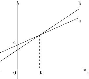
Since , the function has a negative slope at . Hence, we can choose some , such that . This implies that there exists a and a such that for every ,
| (27) |
as illustrated in Fig. 11. Returning to Eq. (23),
| (28) |
From Eq. (28), . Since this inequality holds for any , we let as follows:
| (29) |
Next, we find the lower bound. For some , a sufficient condition for the battery to be empty at some time slot in the interval is that,
| (30) |
We can lower bound using the union bound,
| (31) |
We also have
| (32) |
We define, . Consequently,
Now, for all . Applying the Gärtner-Ellis Theorem, we get,
| (33) |
Combining Eqs. (31) and (33), we have,
| (34) |
Lemma 3.
The asymptotic variance of , satisfies
| (36) |
Proof:
First, we define . The Taylor series expansion of about gives,
Rearranging the terms, we have
| (37) |
Differentiating with respect to , we have,
As , the above expression reduces to,
| (38) |
Substituting in Eq. (38), we have the required result. ∎
Next we show that with the scheme achieves an average utility such that . The instantaneous utility is zero with an probability. For the remaining time, the utility alternates between and as illustrated in Fig. 2. Noting that is an analytic function on the non-negative real line, the Taylor series expansion of the utility function about will be,
and,
We define as the fraction of time that and as the fraction of time that . The average utility can be written as,
| (41) |
where Eq. (41) follows from the fact that and where .
From conservation of energy, the replenishment energy is consumed completely except for the amount lost due to battery overflows. Thus,
| (42) |
where is the probability of the battery being full under the energy management scheme . By a trivial extension of Lemmas 2 and 3, it can be shown that . We can simplify Eq. (42) as,
| (43) |
By substituting Eq. (43) in the first-order term of Eq. (41), we observe that the scheme achieves . Choosing in Eq. (4) completes the proof of Theorem 1.
Appendix C Proof of Theorem 2
Consider any ergodic energy management scheme that uses units of energy in the time slot . Note that scheme can be deterministic or randomized. The asymptotic semi-invariant log moment generating function of the net battery drift is given by . First, we state a lemma that gives the discharge probability scaling for scheme .
Lemma 4.
The probability of battery discharge under Scheme with battery size follows , where is the positive root of .
Proof:
This lemma gives the rate of decay of the probability of complete discharge with respect to the battery size . To prove this result, we first find an upper bound for the required probability. We fix a constant and decompose the time line into intervals, such that each interval is of length and the th interval ends at time slot . Next, define as the event that the battery is empty at the end of time slot 0 and the last time the battery was full (i.e., ) is some time during the interval . The event of an empty battery at time slot 0 can be decomposed as a union of events ,
| (44) |
A necessary condition for event to occur is,
| (45) |
Using Chernoff’s bound, for any ,
| (46) |
where as .
In order to find the tightest bound for each , we choose to maximize , and define . We can rewrite as,
Since , the function has a negative slope at . Hence, we can choose some , such that . This implies that there exists a and a such that for every (see Fig. 11 for a graphical proof),
| (47) |
Next, we find the lower bound. For some , a sufficient condition for the battery to be empty at some time slot in the interval is that,
| (51) |
We can lower bound using the union bound,
| (52) |
We define, . Consequently,
Now, for all . Applying the Gärtner-Ellis Theorem, we get,
| (53) |
where is the asymptotic semi-invariant log-moment generating function of . By noting that Eq. (53) holds for all and combining it with Eq. (52), we have,
| (54) |
Note that exists66 6 Since and , will exist. if and only if . Therefore, for to decay exponentially with , we require,
| (56) |
On the other hand, if , there exists no rate at which the battery discharge probability decays exponentially with , i.e., for all . By substituting in Lemma 4, we get the required scaling law .
Appendix D Proof of Theorem 3
As discussed in Section III-B, our proof is constructive. We use the energy management scheme given in Eq. (8).
We find the individual probabilities in the following lemmas.
Lemma 5.
For the energy management scheme , given any , .
Proof:

First, consider a process that is formed by splicing together the intervals during which the process is above the buffer state . Fig. 12 illustrates a sample path of the process and the corresponding . We denote the diffusion limit of and by and , respectively. While is not a Brownian motion due to its state-dependent drift, will be a Brownian motion in the large-battery regime, with reflections at and unbounded from above as detailed in Step (T1). We assume the starting state of to be . Note that due to the strong Markovian property of a Brownian motion [24], the instants at which the process returns to state (i.e., ) is probabilistically equal to the starting state. Hence we can study these renewal epochs77 7 If we assume the starting state to be , we can simply consider the process to be a delayed renewal process. The steady state properties in the resulting analysis will not change. to obtain steady state properties for the data queue process.
If we define a unit reward (i.e., ) for every time that the process then,
| (58) |
From renewal-reward theory [24] we can write,
| (59) |
where is the expected award accumulated in one renewal period, and is the expected length of the renewal period. To get the correct expression for , we need to write the expressions for and carefully. We define as the expected time for process to return to given that it starts at . The expression for is given by [25],
| (60) |
Similarily, we define as the probability of reaching before starting at . Passing the limit will give the expected reward accumulated in one renewal period. Applying the expression for this probability from [25],
| (61) |
Dividing Eqs. (61) by (60) and passing the limit , we have,
| (62) |
Evaluating the limit , and noting that the overflow probability for the process will be an upper bound on the overflow probability of process , for large we have,
| (63) |
By choosing , we have,
| (64) |
∎Note that Lemma 5 implies that given any , there exists an energy management scheme that achieves an overflow probability . Following the discussion in Step (T1), this implies that for some , .
Lemma 6.
For the energy management scheme , , where is the inverse of the analytic rate-power function .
Proof:
Recall that is not a Brownian motion, but merely the process obtained by applying the diffusion limit on the battery process . In order to evaluate , for scheme , we introduce a new energy management scheme , which allocates an amount of energy identical to: for all . Further, even when , Scheme uses up energy to transmit dummy bits. Thus, the drift of the associated battery state is a constant, completely independent of the queue state. Hence, the diffusion limit for the associated battery process yields a reflected Brownian motion with a single barrier at (recall that the lower barrier was removed). We denote this Brownian limit by . For the same energy replenishment process , the net battery drift is defined as , for a given scheme . We know for all sample paths that, the net drifts satisfy:
| (65) |
for all . The battery underflow probability for scheme is given by . It follows from Eq. (65) that,
| (66) |
The Brownian limit is an exponentially distributed random variable, and the underflow probability is given by [26],
| (67) |
Note that, from the Taylor series expansion of the analytic rate-power function , we have,
| (68) |
Since as , we have Using this observation and combining Eqs. (66) and (67) we have,
| (69) |
completing the proof. Note that, we have in the heavy traffic limit. ∎
Finally, we focus on the average utility of the energy management scheme . The instantaneous utility will be zero when the queue is empty or when the battery is discharged. Since , the contribution of the discharge term can be ignored, since it is a 0-probability event under the large battery regime. For the scheme , the calculation of the average utility becomes exactly the same problem as that for the energy management scheme , which was analyzed in Appendix B. Here, we replace with and the battery size with the data buffer size to get,
| (70) |
We repeat the proof here for completeness. Noting that is an analytic function on the non-negative real line, the Taylor series expansion of the utility function about will be,
and,
We define as the fraction of time that and as the fraction of time that . The average utility can be written as,
| (71) |
where is the probability of the data buffer being empty under the scheme . Eq. (71) follows from the fact that , while Lemmas 2 and 3 yield where .
The average utility can be written as,
| (72) | ||||
| (73) |
where Eq. (72) follows since for some and is an analytic function on the non-negative real line, and Eq. (73) comes from choosing . This completes the proof of Theorem 3.
From conservation of data, the incoming data is transmitted completely except for the amount lost due to data buffer overflows. Thus,
| (74) |
By an extension of Lemmas 2 and 3, it can be shown that . We can simplify Eq. (74) as,
| (75) |
By substituting Eq. (75) in the first-order term of Eq. (71), we observe that the scheme achieves . This completes the proof of Theorem 3.
Appendix E Proof for Theorem 4
The proof of this theorem is constructive. We use the energy management scheme , given in Eq. 15. With this scheme, the mean drifts for the battery state and the data queue state are given by and , respectively. Since the limiting regime for the load is , and hence . As a result, both the battery and the data queue will operate in the heavy traffic limit and we can apply the diffusion limits on these processes to obtain the required probability decay exponents.
In the diffusion limit [21, 26], the decay rate for the discharge probability, , for this energy management scheme can be calculated as,
| (76) |
where the decay exponent is found via the direct application of Theorem 7.1 in Chapter 10 of [26]. With an identical approach, by applying the diffusion limit to the data buffer process and substituting , we can find the decay rate for the buffer overflow probability, as,
| (77) |
Acknowledgment
We thank the associate editor, Professor Lachlan Andrew for his valuable feedback and guidance throughout the review process.
References
- [1] C. Hartung, R. Han, C. Seielstad, and S. Holbrook, “FireWxNet: A Multi-Tiered Portable Wireless System for Monitoring Weather Conditions in Wildland Fire Environments,” in Proc. MobiSys’06, June 2006, pp. 28–41.
- [2] K. Martinez, R. Ong, and J. Hart, “Glacsweb: A Sensor Network for Hostile Environments,” in Proc. IEEE SECON’04, Santa Clara, CA, October 2004, pp. 81– 87.
- [3] A. Kansal and M. B. Srivastava, “An Environmental Energy Harvesting Framework for Sensor Networks,” in Proc. ISLPED’03, August 2003, pp. 481–486.
- [4] S. Meninger, J. O. Mur-Miranda, R. Amirtharajah, A. Chandrakasan, and J. H. Lang, “Vibration-to-electric energy conversion,” IEEE Trans. VLSI Syst., vol. 9, no. 1, pp. 64–76, Feb. 2001.
- [5] J. A. Paradiso and M. Feldmeier, “A Compact, Wireless, Self-Powered Pushbutton Controller,” in Proc. Ubicomp’01. Springer-Verlag, October 2001, pp. 299–304.
- [6] J. M. Rabaey, M. J. Ammer, J. L. da Silva, D. Patel, and S. Roundy, “PicoRadio Supports Ad Hoc Ultra-Low Power Wireless Networking,” IEEE Computer, vol. 33, no. 7, pp. 42–48, 2000.
- [7] W. Weber, “Ambient Intelligence: Industrial Research on a Visionary Concept,” in Proc. ISLPED’03, August 2003, pp. 247–251.
- [8] V. Raghunathan, A. Kansal, J. Hsu, J. Friedman, and M. B. Srivastava, “Design Considerations for Solar Energy Harvesting Wireless Embedded Systems,” in Proc. IEEE IPSN’05, Los Angeles, USA, April 2005, pp. 457 – 462.
- [9] K. Kar, A. Krishnamurthy, and N. Jaggi, “Dynamic Node Activation in Networks of Rechargeable Sensors,” IEEE/ACM Trans. Networking, vol. 14, no. 1, pp. 15–26, Feb. 2006.
- [10] M. Gatzianas, L. Georgiadis, and L. Tassiulas, “Control of wireless networks with rechargeable batteries,” IEEE Trans. Wireless Commun., vol. 9, no. 2, pp. 581–593, Feb. 2010.
- [11] R.-S. Liu, P. Sinha, and C. E. Koksal, “Joint Energy Management and Resource Allocation in Rechargeable Sensor Networks,” in Proc. IEEE INFOCOM’10, San Diego, USA, March 2010.
- [12] O. Ozel and S. Ulukus, “Information-Theoretic Analysis of an Energy Harvesting Communication System,” in Proc. IEEE PIMRC’10, Instanbul, Turkey, September 2010, pp. 330–335.
- [13] A. Kansal, J. Hsu, S. Zahedi, and M. B. Srivastava, “Power Management in Energy Harvesting Sensor Networks,” ACM Trans. Embed. Comput. Syst., vol. 6, no. 4, p. 32, September 2007.
- [14] C. M. Vigorito, D. Ganesan, and A. G. Barto, “Adaptive Control of Duty Cycling in Energy-Harvesting Wireless Sensor Networks,” in Proc. IEEE SECON’07, San Diego, CA, June 2007, pp. 21–30.
- [15] V. Sharma, U. Mukherji, V. Joseph, and S. Gupta, “Optimal energy management policies for energy harvesting sensor nodes,” IEEE Trans. Wireless Commun., vol. 9, no. 4, pp. 1326–1336, April 2010.
- [16] C. K. Ho and R. Zhang, “Optimal Energy Allocation for Wireless Communications Powered by Energy Harvesters,” in Proc. IEEE ISIT’10, June 2010, pp. 2368–2372.
- [17] D. Tse, R. G. Gallager, and J. N. Tsitsiklis, “Optimal Buffer Control for Variable-Rate Lossy Compression,” in Proc. 31st Allerton Conf. Commun. Control and Comput., Allerton, USA, September 1993.
- [18] T. M. Cover and J. A. Thomas, Elements of Information Theory, 1st ed. John Wiley and Sons, 1999.
- [19] J. M. Harrison and R. J. Williams, “Multidimensional reflected brownian motions having exponential stationary distributions,” Ann. Prob., vol. 15, no. 1, pp. 115–137, January 1987.
- [20] H. S. Kim and N. B. Shroff, “On the Asymptotic Relationship between the Overflow Probability and the Loss Ratio,” Adv. Appl. Prob., vol. 33, no. 4, pp. 810–835, December 2001.
- [21] W. Whitt, Stochastic-Process Limits, 1st ed. Springer, 2002.
- [22] Measurement and Instrumentation Data Center. National Renewable Energy Laboratory. [Online]. Available: http://www.nrel.gov/midc/
- [23] W. Rudin, Principles of Mathematical Analysis, 3rd ed. McGraw-Hill, 1976.
- [24] J. M. Harrison, Brownian Motion and Stochastic Flow Systems, 1st ed. John Wiley and Sons, 1985.
- [25] S. M. Ross, Stochastic Processes, 2nd ed. Wiley, 1995.
- [26] S. Asmussen, Applied Probability and Queues, 2nd ed. Springer, 2003.
![[Uncaptioned image]](1009.0569v3/srivastava2.png) |
Rahul Srivastava received the B.Tech. degree in electrical engineering from the Indian Institute of Technology, Madras, India, the M.S. degree in electrical and computer engineering from Rice University, Houston, USA, and the Ph.D. degree in electrical and computer engineering from the Ohio State University, Columbus, USA in 2002, 2005, and 2010 respectively. He is currently working as a Staff Scientist in the Wireless Connectivity Group at the Broadcom Corporation, Sunnyvale, USA. His research interests include wireless communications, communication networks, stochastic processes, and optimization theory. |
![[Uncaptioned image]](1009.0569v3/koksal_photo.png) |
Can Emre Koksal received the B.S. degree in electrical engineering from the Middle East Technical University, Ankara, Turkey, in 1996, and the S.M. and Ph.D. degrees from the Massachusetts Institute of Technology (MIT), Cambridge, in 1998 and 2002, respectively, in electrical engineering and computer science. He was a Postdoctoral Fellow in the Networks and Mobile Systems Group in the Computer Science and Artificial Intelligence Laboratory, MIT, until 2003 and a Senior Researcher jointly in the Laboratory for Computer Communications and the Laboratory for Information Theory at EPFL, Lausanne, Switzerland, until 2006. Since then, he has been an Assistant Professor in the Electrical and Computer Engineering Department, Ohio State University, Columbus, Ohio. His general areas of interest are wireless communication, communication networks, information theory, stochastic processes, and financial economics. He is the recipient of the National Science Foundation CAREER Award in 2011, the OSU College of Engineering Lumley Research Award in 2011, and the co-recipient of an HP Labs - Innovation Research Award in 2011. |