Geometric continuity and compatibility conditions
for 4-patch surfaces

Bo I Johansson Note: Department of Mathematical Sciences, Chalmers University of Technology Note: Department of Mathematical Sciences, University of Gothenburg

Abstract

When considering regularity of surfaces, it is its geometry that is of interest. Thus, the concept of geometric regularity or geometric continuity of a specific order is a relevant concept. In this paper we discuss necessary and sufficient conditions for a 4-patch surface to be geometrically continuous of order one and two or, in other words, being tangent plane continuous and curvature continuous respectively. The focus is on the regularity at the point where the four patches meet and the compatibility conditions that must appear in this case. In this article the compatibility conditions are proved to be independent of the patch parametrization, i.e., the compatibility conditions are universal. In the end of the paper these results are applied to a specific parametrization such as Bezier representation in order to generalize a 4-patch surface result by Sarraga.

Keyword: 4-patch surface; tangent plane continuity; curvature continuity; compatibility conditions, Bezier patch.

1 Introduction

In many applications in Computer-Aided Geometric Design (CAGD) and Computer Graphics a surface is composed of several patches, where a patch usually is represented by a Bezier polynomial, B-spline or NURBS. In particular, each patch is as regular as is needed. Thus, when considering smoothness of a surface such as tangent plane continuity or curvature continuity, the lack of regularity may only occur somewhere at a common boundary curve between two or more patches.

Regularity for a surface constituting of two adjacent patches sharing the same common boundary curve, see Figure 1, is a well studied problem. General results for such a 2-patch surface in the case of $G^{1}$ as well as $G^{2}$ continuity, i.e., tangent plane continuity and curvature continuity respectively, were given by Juergen Kahmann in a paper from 1983, see [7]. In the same paper he applies these results to the case of Bezier patches. Other authors such as Degen [3], Liu and Hoschek [10], Liu [9], DeRose [4], have also treated tangent plane continuity in the 2-patch case. In the case of curvature continuity of 2-patch surface we refer to articles by Kiciak [8], Ye, Liang and Nowacki [20].

A more complicated situation is regularity of a surface consisting of four patches where every pair of adjacent patches meet at a common boundary curve and all the patches intersect at a common vertex, see Figure 2. Among the many authors that have treated regularity problem in this 4-patch surface case are Bézier [1], Sarraga [16], [17] and [18], Ye and Nowacki [21]. Further references and an overview can be found in the book by Hoschek and Lasser [6]. In refered articles so far there have only been considered certain cases of parametric patches, not a general parametrization as is done in this paper. A general approach has also been done by Peters, see the articles by Peters [12]–[15] and by Ye [19].

A general approach to study regularity for a 4-patch surface has been to restrict the patch parametrization to a certain explicit polynomial or rational basis. In this paper we consider 4-patch surfaces where the patches are given by any function of the form $(u,v)\mapsto\mathbf{r}(u,v)\in\mathbb{R}^{3},\,\,u,v\in[0,1]$ . We present necessary and sufficient compatibility conditions in order to have tangent plane continuity and curvature continuity respectively for ´such surfaces. The results we achieve in this paper are independent of the patch parametrization. Thus, these results are of a general nature and can be applied to any parametrization.

In the last section of this paper we apply our results by considering the Sarraga case of filling a hole of a $G^{1}$ -surface in such a way that the extended surface preserves the $G^{1}$ -regularity, see Sarraga [16]. Compared to Sarragas result we reduce the bi-degree to (5,5) of the created interior patch. More generally, we give necessary and sufficient conditions in order to create such an interior patch.

2 Geometric continuity of order 1

When discussing regularity of a surface our focus is on the geometry of the surface and not on its actual parametrization. Thus the notation of geometric continuity is the concept used in this context. The lowest order of regularity is $G^{0}$ , which means that the surface is connected. Another way to put it is to require that its representation is continuous. The next level of regularity is tangent plane continuity, denoted by $G^{1}$ , which is defined here.

Definition 1

A continuous surface is said to be tangent plane continuous, denoted by $G^{1}$ , if every point on the surface has a unique tangent plane, which varies continuously on the surface. Such a surface is also said to be geometrically continuous of order one.

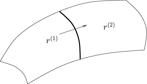
Consider Definition 1 in the case of a 2-patch surface $S$ . Here we use the notation $\mathbf{r}\in C^{1}_{\#}$ for a patch described by a continuous differential function $(u,v)\mapsto\mathbf{r}(u,v)\in\mathbb{R}^{3}$ with $0\leq u,v\leq 1$ satisfying $\mathbf{r}_{u}\times\mathbf{r}_{v}\neq 0$ for $0\leq u,v\leq 1$ . Let the two patches be described as $(u,v)\mapsto\mathbf{r}^{(1)}(u,v)$ with $0\leq u,v\leq 1$ , and $(s,t)\mapsto\mathbf{r}^{(2)}(s,t)$ with $0\leq s,t\leq 1$ . Suppose further that each patch is regular enough, i.e., $\mathbf{r}^{(1)},\mathbf{r}^{(2)}\in C^{1}_{\#}$ . In order for the surface $S$ to be tangent plane continuous the only points that do not automatically fulfill the $G^{1}$ -condition are those along the common boundary curve of the two patches, see Figure 1. On this boundary curve we must particularly have $v\mapsto\mathbf{r}^{(1)}(1,v)=\mathbf{r}^{(2)}(0,t(v))$ for $0\leq v\leq 1$ , where $v\mapsto t(v)$ is a regular reparametrization of the interval $[0,1]$ .

Refer to caption — Figure 1: Two patches connected by a common boundary curve

Thus, at a particular boundary point with parameter value $v$ the tangent plane must fulfill

\mbox{span}\{\mathbf{r}^{(1)}_{u}(1,v),\mathbf{r}^{(1)}_{v}(1,v)\}=\mbox{span}\{\mathbf{r}^{(2)}_{s}(0,t(v)),\mathbf{r}^{(2)}_{t}(0,t(v))\}.

Let us formulate this in an alternative way, where we use the notation $\mathbf{r}^{(2)}(u,v)=\mathbf{r}^{(2)}(u,t(v))$ for $0\leq u,v\leq 1$ . The statement can be found in e. g. [20] and is summarized in the next Lemma.

Lemma 1

A necessary and sufficient condition for two adjacent $C^{1}_{\#}$ -patches $\mathbf{r}^{(1)}$ and $\mathbf{r}^{(2)}$ joining $G^{1}$ -continuously along its common boundary curve $v\mapsto\mathbf{r}^{(1)}(1,v)=\mathbf{r}^{(2)}(0,v)$ is that there exist continuous functions $\lambda_{1,2}$ and $\kappa_{1,2}$ such that

\mathbf{r}^{(2)}_{u}(0,v)=\lambda_{1,2}(v)\,\mathbf{r}^{(1)}_{u}(1,v)+\kappa_{1,2}(v)\,\mathbf{r}^{(1)}_{v}(1,v),\,\,\,\,0\leq v\leq 1.

(2.1)

In this paper we will consider the problem of a surface constituting of four patches where every two adjacent patches have a common boundary curve, see Figure 2. Moreover, the four patches intersect at a common vertex $V$ . In the case of a 4-patch surface being $G^{1}$ we will prove that there must exist compatibility conditions at the intersection point $V$ . The compatibility conditions can be rephrased in such a way that we formulate necessary and sufficient conditions on the functions $\lambda_{ij}$ and $\kappa_{ij}$ at the intersection point $V$ .

First, by using the relation (2.1) we get the next four relations between the patches $(1)$ – $(2)$ , $(2)$ – $(3)$ , $(4)$ – $(3)$ and $(1)$ – $(4)$ . We use the same parameters $u$ and $v$ for all the patches, where $0\leq u,v\leq 1$ . Thus

\begin{split}\mathbf{r}^{(2)}_{u}(0,v)&=\lambda_{1,2}(v)\mathbf{r}^{(1)}_{u}(1,v)+\kappa_{1,2}(v)\mathbf{r}^{(1)}_{v}(1,v)\\ \mathbf{r}^{(3)}_{u}(0,v)&=\lambda_{4,3}(v)\mathbf{r}^{(4)}_{u}(1,v)+\kappa_{4,3}(v)\mathbf{r}^{(4)}_{v}(1,v)\end{split}

(2.2)

and

\begin{split}\mathbf{r}^{(4)}_{v}(u,0)&=\lambda_{1,4}(u)\mathbf{r}^{(1)}_{v}(u,1)+\kappa_{1,4}(u)\mathbf{r}^{(1)}_{u}(u,1)\\ \mathbf{r}^{(3)}_{v}(u,0)&=\lambda_{2,3}(u)\mathbf{r}^{(2)}_{v}(u,1)+\kappa_{2,3}(u)\mathbf{r}^{(2)}_{u}(u,1).\end{split}

(2.3)

We have here used a patch numbering as is indicated in Figure 2.

Considering a tangent plane continuous 4-patch surface, it must satisfy that every pair of its patches with a common boundary curve coincide along that curve. The same must be true of its derivatives along the same boundary curve.

Thus

\left.\begin{array}[]{l}\mathbf{r}^{(1)}_{v}(1,v)=\mathbf{r}^{(2)}_{v}(0,v)\\ \mathbf{r}^{(4)}_{v}(1,v)=\mathbf{r}^{(3)}_{v}(0,v),\,v\in[0,1]\end{array}\right.

(2.4)

and

\left.\begin{array}[]{l}\mathbf{r}^{(1)}_{u}(u,1)=\mathbf{r}^{(4)}_{u}(u,0)\\ \mathbf{r}^{(2)}_{u}(u,1)=\mathbf{r}^{(3)}_{u}(u,0),\,u\in[0,1].\end{array}\right.

(2.5)

Using the equations (2.2)–(2.5), we prove the next theorem, which is the main result in this section. In the case where the patches are described by polynomials, this result has already been published by Bézier in 1986. See [1], p 44-46. Here we formulate and prove the result for a general parametrization.

Theorem 1

Let $S$ be a 4-patch surface consisting of $C^{1}_{\#}$ -patches $\mathbf{r}^{(i)}$ , $i=1,\ldots,4$ . Let $V$ be the intersection point of the four patches. Then, necessary and sufficient conditions in order for the surface $S$ to be tangent plane continuous are that there exist continuous functions $\lambda_{ij}$ and $\kappa_{ij}$ , $i=1,j=2,4$ and $i=2,4,j=3$ , satisfying the equations (2.2) and (2.3), and the following relations

\begin{array}[]{l}\kappa_{1,2}=\lambda_{1,4}\,\kappa_{4,3}\\ \kappa_{1,4}=\lambda_{1,2}\,\kappa_{2,3}\end{array}

(2.6)

and

\begin{array}[]{l}\lambda_{1,2}-\lambda_{4,3}=\kappa_{1,4}\,\kappa_{4,3}\\ \lambda_{1,4}-\lambda_{2,3}=\kappa_{1,2}\,\kappa_{2,3}\end{array}

(2.7)

at the vertex $V$ .

Remark. The notations $\kappa_{1,2}$ , $\lambda_{1,4}$ , $\kappa_{4,3}$ , etc, are to be interpreted as $\kappa_{1,2}(1)$ , $\lambda_{1,4}(1)$ , $\kappa_{4,3}(0)$ , etc. i.e., as the value of the functions at the vertex $V$ .

Proof.

In order to prove the above statement, we must see under what conditions the equations (2.2) and (2.3) are all satisfied at the vertex $V$ . We use here the short notation $\mathbf{r}^{(1)}_{u}$ for $\mathbf{r}^{(1)}_{u}(u,v)|_{V}=\mathbf{r}^{(1)}_{u}(1,1)$ , etc.

We start by eliminating $\mathbf{r}^{(2)}_{u}$ , $\mathbf{r}^{(2)}_{v}$ , $\mathbf{r}^{(4)}_{u}$ and $\mathbf{r}^{(4)}_{v}$ in the equations (2.2) and (2.3) by using (2.4) and (2.5) to get

\left.\begin{array}[]{rrrrl}\lambda_{1,2}\mathbf{r}^{(1)}_{u}&+\,\kappa_{1,2}\mathbf{r}^{(1)}_{v}&-\,\mathbf{r}^{(3)}_{u}&&=0\\ \lambda_{4,3}\mathbf{r}^{(1)}_{u}&&-\,\mathbf{r}^{(3)}_{u}&+\,\kappa_{4,3}\mathbf{r}^{(3)}_{v}&=0\\ \kappa_{1,4}\mathbf{r}^{(1)}_{u}&+\,\lambda_{1,4}\mathbf{r}^{(1)}_{v}&&-\,\mathbf{r}^{(3)}_{v}&=0\\ &\lambda_{2,3}\mathbf{r}^{(1)}_{v}&+\,\kappa_{2,3}\mathbf{r}^{(3)}_{u}&-\,\mathbf{r}^{(3)}_{v}&=0.\end{array}\right.

(2.8)

With the use of (2.8) we replace the second and fourth equation in the above system by eliminating $\mathbf{r}^{(3)}_{u}$ and $\mathbf{r}^{(3)}_{v}$ to get

\left.\begin{array}[]{l}(\lambda_{4,3}-\lambda_{1,2}+\kappa_{1,4}\kappa_{4,3})\mathbf{r}^{(1)}_{u}+(\lambda_{1,4}\kappa_{4,3}-\kappa_{1,2})\mathbf{r}^{(1)}_{v}=0\\ (\lambda_{1,2}\kappa_{2,3}-\kappa_{1,4})\mathbf{r}^{(1)}_{u}+(\lambda_{2,3}-\lambda_{1,4}+\kappa_{1,2}\kappa_{2,3})\mathbf{r}^{(1)}_{v}=0.\end{array}\right.

Since the vectors $\mathbf{r}^{(1)}_{u},\mathbf{r}^{(1)}_{v}$ span the tangent plane, it follows from the above equations that (2.6) and (2.7) must hold. This concludes the proof. $\square$

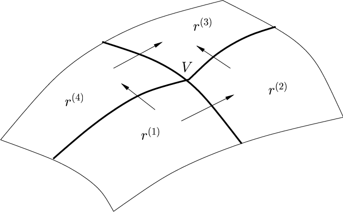
Let us look at some simple consequences of Theorem 1. Obviously, the functions $\lambda_{ij}$ are not allowed to be zero if tangential continuity is to be satisfied. Thus, if e.g. $\kappa_{4,3}(0)\neq 0$ then $\kappa_{1,2}(1)\neq 0$ , which follows from (2.6). On the other hand, if $\kappa_{1,4}(1)=0$ then also $\kappa_{2,3}(0)=0$ . This situation is exemplified in Figure 3. In general, it follows from equation (2.6) that the pair of $\kappa_{ij}$ ’s in each equality must both be zero or non-zero.

Another observation that can be done from (2.6) and (2.7) is that the next relations are true

\begin{split}\lambda_{1,4}\lambda_{4,3}&=\lambda_{1,4}(\lambda_{1,2}-\kappa_{1,4}\kappa_{4,3})=\lambda_{1,2}\lambda_{1,4}-\lambda_{1,4}\kappa_{4,3}\kappa_{1,4}\\ &=\lambda_{1,2}\lambda_{1,4}-\kappa_{1,2}\kappa_{1,4}\end{split}

and

\begin{split}\lambda_{1,2}\lambda_{2,3}&=\lambda_{1,2}(\lambda_{1,4}-\kappa_{1,2}\kappa_{2,3})=\lambda_{1,2}\lambda_{1,4}-\kappa_{1,2}\lambda_{1,2}\kappa_{2,3}\\ &=\lambda_{1,2}\lambda_{1,4}-\kappa_{1,2}\kappa_{1,4}.\end{split}

In particular, we have

\lambda_{1,2}\lambda_{2,3}=\lambda_{1,4}\lambda_{4,3},

(2.9)

which will be useful in the next section.

3 Geometric continuity of order 2

In this section we consider 4-patch surfaces of higher regularity. Therefore we introduce the following concept.

Definition 2

A tangent plane continuous, $G^{1}$ , surface is said to be curvature continuous, denoted by $G^{2}$ , if every point on the surface has a unique Dupin indicatrix, which varies continuously on the surface. Such a surface is also said to be geometrically continuous of order two.

Another equivalent way to describe the notation of curvature continuity is to say that the normal curvature at each point and in each tangential direction¹¹ 1 In fact, it is enough that it holds for 3 pairwise linearly independent tangential directions by the 3-Tangent Theorem, see Pegna & Wolter [11] or Hoschek & Lasser [6], p 333. has to be unique, or the principal curvatures are unique. These differential geometric notations are introduced and explained in any book about differential geometry, e.g. [2]. First we consider a 2-patch surface, where the patches are of regularity $C^{2}_{\#}=C^{1}_{\#}\cap C^{2}$ . Thus, lack of $G^{2}$ -regularity for the surface $S$ can only occur at the common boundary of the two patches. A necessary and sufficient condition for a 2-patch surface to be curvature continuous can be found in a paper by Juergen Kahmann [7]. A proof of this well-known result can also be found in [20]. The result is summarized in the next Lemma.

Lemma 2

Let $S$ be a 2-patch surface consisting of the $C^{2}_{\#}$ -patches $(u,v)\mapsto\mathbf{r}^{(1)}(u,v)$ and $(u,v)\mapsto\mathbf{r}^{(2)}(u,v)$ , $0\leq u,v\leq 1$ , satisfying equation (2.1) along their common boundary curve. A necessary and sufficient condition for the surface $S$ to be curvature continuous is that the following relation is fulfilled

\begin{split}\mathbf{r}^{(2)}_{uu}(0,v)&=\lambda^{2}_{1,2}(v)\mathbf{r}^{(1)}_{uu}(1,v)+2\lambda_{1,2}(v)\kappa_{1,2}(v)\mathbf{r}^{(1)}_{uv}(1,v)+\kappa^{2}_{1,2}(v)\mathbf{r}^{(1)}_{vv}(1,v)\\ &+\mu_{1,2}(v)\mathbf{r}^{(1)}_{u}(1,v)+\nu_{1,2}(v)\mathbf{r}^{(1)}_{v}(1,v),\,\,\,\,\mbox{$0\leq v\leq 1$,}\end{split}

(3.10)

where the functions $\lambda_{1,2}$ , $\kappa_{1,2}$ , $\mu_{1,2}$ and $\nu_{1,2}$ are continuous.

We now continue to consider a 4-patch surface as shown in Figure 2. The first and most obvious conditions to have geometric continuity of order two are that the equations in (2.2) and (2.3) are still satisfied when differentiated with respect to the parameters $u$ and $v$ respectively. We assume here that the functions $\lambda_{ij}$ and $\kappa_{ij}$ are differentiable. Thus

\begin{split}&\mathbf{r}^{(2)}_{uv}(0,v)=\lambda^{\prime}_{1,2}(v)\,\mathbf{r}^{(1)}_{u}(1,v)+\lambda_{1,2}(v)\,\mathbf{r}^{(1)}_{uv}(1,v)+\kappa^{\prime}_{1,2}(v)\,\mathbf{r}^{(1)}_{v}(1,v)+\kappa_{1,2}(v)\,\mathbf{r}^{(1)}_{vv}(1,v)\\ &\mathbf{r}^{(3)}_{uv}(0,v)=\lambda^{\prime}_{4,3}(v)\,\mathbf{r}^{(4)}_{u}(1,v)+\lambda_{4,3}(v)\,\mathbf{r}^{(4)}_{uv}(1,v)+\kappa^{\prime}_{4,3}(v)\,\mathbf{r}^{(4)}_{v}(1,v)+\kappa_{4,3}(v)\,\mathbf{r}^{(4)}_{vv}(1,v)\end{split}

(3.11)

and

\begin{split}&\mathbf{r}^{(4)}_{vu}(u,0)=\lambda^{\prime}_{1,4}(u)\,\mathbf{r}^{(1)}_{v}(u,1)+\lambda_{1,4}(u)\,\mathbf{r}^{(1)}_{vu}(u,1)+\kappa^{\prime}_{1,4}(u)\,\mathbf{r}^{(1)}_{u}(u,1)+\kappa_{1,4}(u)\,\mathbf{r}^{(1)}_{uu}(u,1)\\ &\mathbf{r}^{(3)}_{vu}(u,0)=\lambda^{\prime}_{2,3}(u)\,\mathbf{r}^{(2)}_{v}(u,1)+\lambda_{2,3}(u)\,\mathbf{r}^{(2)}_{vu}(u,1)+\kappa^{\prime}_{2,3}(u)\,\mathbf{r}^{(2)}_{u}(u,1)+\kappa_{2,3}(u)\,\mathbf{r}^{(2)}_{uu}(u,1)\end{split}

(3.12)

must hold. From Lemma 2, we know that curvature continuity implies that the next four relations must be fulfilled

\begin{split}\mathbf{r}^{(2)}_{uu}(0,v)&=\lambda^{2}_{1,2}(v)\mathbf{r}^{(1)}_{uu}(1,v)+2\lambda_{1,2}(v)\kappa_{1,2}(v)\mathbf{r}^{(1)}_{uv}(1,v)+\kappa^{2}_{1,2}(v)\mathbf{r}^{(1)}_{vv}(1,v)\\ &\makebox[11.38109pt]{\ }+\mu_{1,2}(v)\mathbf{r}^{(1)}_{u}(1,v)+\nu_{1,2}(v)\mathbf{r}^{(1)}_{v}(1,v)\end{split}

(3.13)

\begin{split}\mathbf{r}^{(3)}_{uu}(0,v)&=\lambda^{2}_{4,3}(v)\mathbf{r}^{(4)}_{uu}(1,v)+2\lambda_{4,3}(v)\kappa_{4,3}(v)\mathbf{r}^{(4)}_{uv}(1,v)+\kappa^{2}_{4,3}(v)\mathbf{r}^{(4)}_{vv}(1,v)\\ &\makebox[11.38109pt]{\ }+\mu_{4,3}(v)\mathbf{r}^{(4)}_{u}(1,v)+\nu_{4,3}(v)\mathbf{r}^{(4)}_{v}(1,v)\end{split}

(3.14)

and

\begin{split}\mathbf{r}^{(3)}_{vv}(u,0)&=\lambda^{2}_{2,3}(u)\mathbf{r}^{(2)}_{vv}(u,1)+2\lambda_{2,3}(u)\kappa_{2,3}(u)\mathbf{r}^{(2)}_{uv}(u,1)+\kappa^{2}_{2,3}(u)\mathbf{r}^{(2)}_{uu}(u,1)\\ &\makebox[11.38109pt]{\ }+\mu_{2,3}(u)\mathbf{r}^{(2)}_{v}(u,1)+\nu_{2,3}(u)\mathbf{r}^{(2)}_{u}(u,1)\end{split}

(3.15)

\begin{split}\mathbf{r}^{(4)}_{vv}(u,0)&=\lambda^{2}_{1,4}(u)\mathbf{r}^{(1)}_{vv}(u,1)+2\lambda_{1,4}(u)\kappa_{1,4}(u)\mathbf{r}^{(1)}_{uv}(u,1)+\kappa^{2}_{1,4}(u)\mathbf{r}^{(1)}_{uu}(u,1)\\ &\makebox[11.38109pt]{\ }+\mu_{1,4}(u)\mathbf{r}^{(1)}_{v}(u,1)+\nu_{1,4}(u)\mathbf{r}^{(1)}_{u}(u,1).\end{split}

(3.16)

The main result of this section is a general result. It concerns parameterized patches of any kind and it is formulated next.

Theorem 2

Let $S$ be a $G^{1}$ 4-patch surface consisting of $C^{2}_{\#}$ -patches $\mathbf{r}^{(i)}$ , $i=1,\ldots,4$ . Let $V$ be the intersection point of the four patches. Then, necessary and sufficient conditions in order for the surface $S$ to be curvature continuous are that there exist continuously differentiable functions $\lambda_{ij}$ and $\kappa_{ij}$ and continuous functions $\mu_{ij}$ and $\nu_{ij}$ , $i=1,j=2,4$ and $i=2,4,j=3$ , satisfying the equations (3.13)–(3.16) and that the following relations

		$\displaystyle 2\lambda_{4,3}\lambda^{\prime}_{1,4}\kappa_{4,3}-\nu_{1,2}+\nu_{4,3}\lambda_{1,4}+\mu_{1,4}\kappa^{2}_{4,3}=0$		(3.17)
		$\displaystyle 2\lambda_{2,3}\lambda^{\prime}_{1,2}\kappa_{2,3}-\nu_{1,4}+\nu_{2,3}\lambda_{1,2}+\mu_{1,2}\kappa^{2}_{2,3}=0$
		$\displaystyle 2\lambda_{4,3}\kappa_{4,3}\kappa^{\prime}_{1,4}-\mu_{1,2}+\mu_{4,3}+\nu_{4,3}\kappa_{1,4}+\nu_{1,4}\kappa^{2}_{4,3}=0$
		$\displaystyle 2\lambda_{2,3}\kappa_{2,3}\kappa^{\prime}_{1,2}-\mu_{1,4}+\mu_{2,3}+\nu_{2,3}\kappa_{1,2}+\nu_{1,2}\kappa^{2}_{2,3}=0$
		$\displaystyle\lambda^{\prime}_{4,3}-\lambda_{2,3}\lambda^{\prime}_{1,2}+\lambda_{4,3}\kappa^{\prime}_{1,4}-\lambda_{1,2}\kappa^{\prime}_{2,3}+\kappa_{1,4}\kappa^{\prime}_{4,3}-\mu_{1,2}\kappa_{2,3}+\nu_{1,4}\kappa_{4,3}=0$
		$\displaystyle\lambda^{\prime}_{2,3}-\lambda_{4,3}\lambda^{\prime}_{1,4}+\lambda_{2,3}\kappa^{\prime}_{1,2}-\lambda_{1,4}\kappa^{\prime}_{4,3}+\kappa_{1,2}\kappa^{\prime}_{2,3}-\mu_{1,4}\kappa_{4,3}+\nu_{1,2}\kappa_{2,3}=0$

hold at the vertex $V$ .

Remark. We use here the same short notations as in Theorem 1, i.e., $\lambda_{1,2}$ , $\kappa_{1,2}$ , $\mu_{1,2}$ , $\nu_{1,2}$ etc, are to be interpreted as $\lambda_{1,2}(1)$ , $\kappa_{1,2}(1)$ , $\mu_{1,2}(1)$ , $\nu_{1,2}(1)$ , etc, i.e., as the value of the functions at the vertex $V$ .

Proof

The idea in the proof is to study the equation system consisting of (3.11)–(3.16) and to reduce, as far as possible, the number of equations including derivatives of second order. To simplify the notations in the proof we use $\mathbf{r}^{(1)}_{u}$ for $\mathbf{r}^{(1)}_{u}(u,v)|_{V}=\mathbf{r}^{(1)}_{u}(1,1)$ , etc.

First, we know that the equations (3.11) and (3.12) must hold. Using the relations (2.4) and (2.5) in order to replace the vectors $\mathbf{r}^{(4)}_{u}$ and $\mathbf{r}^{(2)}_{v}$ with $\mathbf{r}^{(1)}_{u}$ and $\mathbf{r}^{(1)}_{v}$ respectively. Combining this with (2.2) and (2.3) in order to eliminate $\mathbf{r}^{(2)}_{u}$ and $\mathbf{r}^{(4)}_{v}$ we get

\begin{split}&\lambda_{1,2}\mathbf{r}^{(1)}_{uv}-\mathbf{r}^{(2)}_{uv}+\lambda^{\prime}_{1,2}\mathbf{r}^{(1)}_{u}+\kappa^{\prime}_{1,2}\mathbf{r}^{(1)}_{v}+\kappa_{1,2}\mathbf{r}^{(1)}_{vv}=0\phantom{.}\\ &\lambda_{4,3}\mathbf{r}^{(4)}_{uv}-\mathbf{r}^{(3)}_{uv}+\lambda^{\prime}_{4,3}\mathbf{r}^{(1)}_{u}+\kappa^{\prime}_{4,3}(\lambda_{1,4}\mathbf{r}^{(1)}_{v}+\kappa_{1,4}\mathbf{r}^{(1)}_{u})+\kappa_{4,3}\mathbf{r}^{(4)}_{vv}=0\phantom{.}\\ &\lambda_{1,4}\mathbf{r}^{(1)}_{vu}-\mathbf{r}^{(4)}_{vu}+\kappa^{\prime}_{1,4}\mathbf{r}^{(1)}_{u}+\lambda^{\prime}_{1,4}\mathbf{r}^{(1)}_{v}+\kappa_{1,4}\mathbf{r}^{(1)}_{uu}=0\phantom{.}\\ &\lambda_{2,3}\mathbf{r}^{(2)}_{vu}-\mathbf{r}^{(3)}_{vu}+\kappa^{\prime}_{2,3}(\lambda_{1,2}\mathbf{r}^{(1)}_{u}+\kappa_{1,2}\mathbf{r}^{(1)}_{v})+\lambda^{\prime}_{2,3}\mathbf{r}^{(1)}_{v}+\kappa_{2,3}\mathbf{r}^{(2)}_{uu}=0.\end{split}

In the above equation system we multiply the first equation by $\lambda_{2,3}$ , the second one with $-1$ , the third one with $-\lambda_{4,3}$ and add them to the fourth equation. We get

	$\displaystyle(-\lambda^{\prime}_{4,3}+\lambda_{2,3}\lambda^{\prime}_{1,2}-\lambda_{4,3}\kappa^{\prime}_{1,4}+\lambda_{1,2}\kappa^{\prime}_{2,3}-\kappa_{1,4}\kappa^{\prime}_{4,3})\mathbf{r}^{(1)}_{u}+(\lambda^{\prime}_{2,3}+\lambda_{2,3}\kappa^{\prime}_{1,2}-\lambda_{4,3}\lambda^{\prime}_{1,4}$		(3.18)
	$\displaystyle\ \ \ \ \ +\kappa_{1,2}\kappa^{\prime}_{2,3}-\lambda_{1,4}\kappa^{\prime}_{4,3})\mathbf{r}^{(1)}_{v}-\lambda_{4,3}\kappa_{1,4}\mathbf{r}^{(1)}_{uu}+\lambda_{2,3}\kappa_{1,2}\mathbf{r}^{(1)}_{vv}+\kappa_{2,3}\mathbf{r}^{(2)}_{uu}-\kappa_{4,3}\mathbf{r}^{(4)}_{vv}=0.$		(3.18)

Considering the last part in the equation (3.18) and using the equations (3.13) and (3.16) it follows that

			$\displaystyle\makebox[-42.67912pt]{\ }-\lambda_{4,3}\kappa_{1,4}\mathbf{r}^{(1)}_{uu}+\lambda_{2,3}\kappa_{1,2}\mathbf{r}^{(1)}_{vv}+\kappa_{2,3}\mathbf{r}^{(2)}_{uu}-\kappa_{4,3}\mathbf{r}^{(4)}_{vv}$
		$\displaystyle=$	$\displaystyle-\lambda_{4,3}\kappa_{1,4}\mathbf{r}^{(1)}_{uu}+\lambda_{2,3}\kappa_{1,2}\mathbf{r}^{(1)}_{vv}$
			$\displaystyle\ \ \ +\kappa_{2,3}(\lambda^{2}_{1,2}\mathbf{r}^{(1)}_{uu}+2\lambda_{1,2}\kappa_{1,2}\mathbf{r}^{(1)}_{uv}+\kappa^{2}_{1,2}\mathbf{r}^{(1)}_{vv}+\mu_{1,2}\mathbf{r}^{(1)}_{u}+\nu_{1,2}\mathbf{r}^{(1)}_{v})$
			$\displaystyle\ \ \ -\kappa_{4,3}(\lambda^{2}_{1,4}\mathbf{r}^{(1)}_{vv}+2\lambda_{1,4}\kappa_{1,4}\mathbf{r}^{(1)}_{uv}+\kappa^{2}_{1,4}\mathbf{r}^{(1)}_{uu}+\mu_{1,4}\mathbf{r}^{(1)}_{v}+\nu_{1,4}\mathbf{r}^{(1)}_{u})$
		$\displaystyle=$	$\displaystyle\kappa_{2,3}(\mu_{1,2}\mathbf{r}^{(1)}_{u}+\nu_{1,2}\mathbf{r}^{(1)}_{v})-\kappa_{4,3}(\mu_{1,4}\mathbf{r}^{(1)}_{v}+\nu_{1,4}\mathbf{r}^{(1)}_{u})$
			$\displaystyle\ \ \ +(\kappa_{2,3}\lambda^{2}_{1,2}-\kappa_{4,3}\kappa^{2}_{1,4}-\lambda_{4,3}\kappa_{1,4})\mathbf{r}^{(1)}_{uu}$
			$\displaystyle\ \ \ +(\kappa_{2,3}\kappa^{2}_{1,2}-\kappa_{4,3}\lambda^{2}_{1,4}+\lambda_{2,3}\kappa_{1,2})\mathbf{r}^{(1)}_{vv}$
			$\displaystyle\ \ \ +2(\kappa_{2,3}\lambda_{1,2}\kappa_{1,2}-\kappa_{4,3}\lambda_{1,4}\kappa_{1,4})\mathbf{r}^{(1)}_{uv}.$

In order to further reduce the above formula, we use the relations (2.6) and (2.7) to get

$\displaystyle\kappa_{2,3}\lambda^{2}_{1,2}-\kappa_{4,3}\kappa^{2}_{1,4}-\lambda_{4,3}\kappa_{1,4}$	$\displaystyle=$	$\displaystyle\kappa_{1,4}\lambda_{1,2}-\kappa_{4,3}\kappa^{2}_{1,4}-\lambda_{4,3}\kappa_{1,4}$
	$\displaystyle=$	$\displaystyle\kappa_{1,4}(\lambda_{1,2}-\lambda_{4,3}-\kappa_{1,4}\kappa_{4,3})=0,$
$\displaystyle\kappa_{2,3}\kappa^{2}_{1,2}-\kappa_{4,3}\lambda^{2}_{1,4}+\lambda_{2,3}\kappa_{1,2}$	$\displaystyle=$	$\displaystyle\kappa_{2,3}\kappa^{2}_{1,2}-\kappa_{1,2}\lambda_{1,4}+\lambda_{2,3}\kappa_{1,2}$
	$\displaystyle=$	$\displaystyle\kappa_{1,2}(\lambda_{2,3}-\lambda_{1,4}+\kappa_{1,2}\kappa_{2,3})=0$
and
$\displaystyle\kappa_{2,3}\lambda_{1,2}\kappa_{1,2}-\kappa_{4,3}\lambda_{1,4}\kappa_{1,4}$	$\displaystyle=$	$\displaystyle\kappa_{1,4}\kappa_{1,2}-\kappa_{1,2}\kappa_{1,4}=0.$

Thus, it follows that

\begin{split}&-\lambda_{4,3}\kappa_{1,4}\mathbf{r}^{(1)}_{uu}+\lambda_{2,3}\kappa_{1,2}\mathbf{r}^{(1)}_{vv}+\kappa_{2,3}\mathbf{r}^{(3)}_{uu}-\kappa_{4,3}\mathbf{r}^{(3)}_{vv}\\ &\phantom{some}=(\kappa_{2,3}\mu_{1,2}-\kappa_{4,3}\nu_{1,4})\mathbf{r}^{(1)}_{u}+(\kappa_{2,3}\nu_{1,2}-\kappa_{4,3}\mu_{1,4})\mathbf{r}^{(1)}_{v}.\end{split}

Input the above equality into the equation (3.18). As before, the independence of the two vectors $\mathbf{r}^{(1)}_{u}$ and $\mathbf{r}^{(1)}_{v}$ gives

\begin{split}-\lambda^{\prime}_{4,3}-\lambda_{4,3}\kappa^{\prime}_{1,4}+\lambda_{2,3}\lambda^{\prime}_{1,2}+\lambda_{1,2}\kappa^{\prime}_{2,3}-\kappa_{1,4}\kappa^{\prime}_{4,3}+\kappa_{2,3}\mu_{1,2}-\kappa_{4,3}\nu_{1,4}=0\hphantom{.}\\ \lambda^{\prime}_{2,3}-\lambda_{4,3}\lambda^{\prime}_{1,4}+\lambda_{2,3}\kappa^{\prime}_{1,2}+\kappa_{1,2}\kappa^{\prime}_{2,3}-\lambda_{1,4}\kappa^{\prime}_{4,3}+\kappa_{2,3}\nu_{1,2}-\kappa_{4,3}\mu_{1,4}=0.\end{split}

(3.19)

The equations in (3.19) are necessary in order to fulfill the condition of geometric continuity of order 2.

Let us next study the equations (3.13)–(3.16) more closely. We rewrite two of these equations. Start with the equation (3.14) by adding to it the first equation in (3.11) multiplied by $2\lambda_{4,3}\,\kappa_{4,3}$ and equation (3.13) multiplied by $-\lambda_{4,3}/\lambda_{1,2}$ . We get the new equation

		$\displaystyle(\mu_{4,3}+2\lambda_{4,3}\kappa_{4,3}\kappa^{\prime}_{1,4}-\mu_{1,2}\frac{\lambda_{4,3}}{\lambda_{1,2}})\mathbf{r}^{(1)}_{u}+(2\lambda_{4,3}\kappa_{4,3}\lambda^{\prime}_{1,4}-\nu_{1,2}\frac{\lambda_{4,3}}{\lambda_{1,2}})\mathbf{r}^{(1)}_{v}+\nu_{4,3}\mathbf{r}^{(3)}_{v}$		(3.20)
		$\displaystyle\makebox[5.69054pt]{\ }+(\lambda^{2}_{4,3}+2\lambda_{4,3}\kappa_{4,3}\kappa_{1,4}-\lambda_{1,2}\lambda_{4,3})\mathbf{r}^{(1)}_{uu}-\kappa^{2}_{1,2}\frac{\lambda_{4,3}}{\lambda_{1,2}}\mathbf{r}^{(1)}_{vv}-(1-\frac{\lambda_{4,3}}{\lambda_{1,2}})\mathbf{r}^{(3)}_{uu}+\kappa^{2}_{4,3}\mathbf{r}^{(3)}_{vv}=0.$		(3.20)

We continue with the equation (3.15). To this one we add the first equation in (3.12) multiplied by $2\lambda_{2,3}\,\kappa_{2,3}$ and equation (3.16) multiplied by $-\lambda_{2,3}/\lambda_{1,4}$ . We have

		$\displaystyle(2\lambda^{\prime}_{1,2}\lambda_{2,3}\kappa_{2,3}-\nu_{1,4}\frac{\lambda_{2,3}}{\lambda_{1,4}})\mathbf{r}^{(1)}_{u}+(\mu_{2,3}+2\kappa^{\prime}_{1,2}\lambda_{2,3}\kappa_{2,3}-\mu_{1,4}\frac{\lambda_{2,3}}{\lambda_{1,4}})\mathbf{r}^{(1)}_{v}+\nu_{2,3}\mathbf{r}^{(3)}_{u}$		(3.21)
		$\displaystyle\makebox[5.69054pt]{\ }-\kappa^{2}_{1,4}\frac{\lambda_{2,3}}{\lambda_{1,4}}\mathbf{r}^{(1)}_{uu}+(\lambda^{2}_{2,3}+2\kappa_{1,2}\lambda_{2,3}\kappa_{2,3}-\lambda_{1,4}\lambda_{2,3})\mathbf{r}^{(1)}_{vv}+\kappa^{2}_{2,3}\mathbf{r}^{(3)}_{uu}-(1-\frac{\lambda_{2,3}}{\lambda_{1,4}})\mathbf{r}^{(3)}_{vv}=0.$		(3.21)

Let us now consider the equation (3.20). We want to rewrite this equation in order to make it easier to handle. Using the relations (2.3)–(2.4), (2.6)–(2.7) combined with (3.13) and (3.16), we get

\begin{split}&(\mu_{4,3}\lambda_{1,2}+2\lambda_{1,2}\lambda_{4,3}\kappa_{4,3}\kappa^{\prime}_{1,4}-\mu_{1,2}\lambda_{4,3})\mathbf{r}^{(1)}_{u}+\lambda_{4,3}(2\lambda_{1,2}\kappa_{4,3}\lambda^{\prime}_{1,4}-\nu_{1,2})\mathbf{r}^{(1)}_{v}+\nu_{4,3}\lambda_{1,2}\mathbf{r}^{(4)}_{v}\\ &\makebox[11.38109pt]{\ }+\lambda_{1,2}\lambda_{4,3}(\lambda_{4,3}+2\kappa_{1,4}\kappa_{4,3}-\lambda_{1,2})\mathbf{r}^{(1)}_{uu}-\lambda_{4,3}\kappa^{2}_{1,2}\mathbf{r}^{(1)}_{vv}-(\lambda_{1,2}-\lambda_{4,3})\mathbf{r}^{(2)}_{uu}+\lambda_{1,2}\kappa^{2}_{4,3}\mathbf{r}^{(4)}_{vv}\\[2.84526pt] &=(\mu_{4,3}\lambda_{1,2}+2\lambda_{1,2}\lambda_{4,3}\kappa_{4,3}\kappa^{\prime}_{1,4}-\mu_{1,2}\lambda_{4,3})\mathbf{r}^{(1)}_{u}+\lambda_{4,3}(2\lambda_{1,2}\kappa_{4,3}\lambda^{\prime}_{1,4}-\nu_{1,2})\mathbf{r}^{(1)}_{v}\\ &\makebox[11.38109pt]{\ }+\nu_{4,3}\lambda_{1,2}(\kappa_{1,4}\mathbf{r}^{(1)}_{u}+\lambda_{1,4}\mathbf{r}^{(1)}_{v})+\lambda_{1,2}\lambda_{4,3}\kappa_{1,4}\kappa_{4,3}\mathbf{r}^{(1)}_{uu}-\lambda_{4,3}\kappa^{2}_{1,2}\mathbf{r}^{(1)}_{vv}-\kappa_{1,4}\kappa_{4,3}(\lambda^{2}_{1,2}\mathbf{r}^{(1)}_{uu}\\ &\makebox[11.38109pt]{\ }+2\lambda_{1,2}\kappa_{1,2}\mathbf{r}^{(1)}_{uv}+\kappa^{2}_{1,2}\mathbf{r}^{(1)}_{vv}+\mu_{1,2}\mathbf{r}^{(1)}_{u}+\nu_{1,2}\mathbf{r}^{(1)}_{v})+\lambda_{1,2}\kappa^{2}_{4,3}(\lambda^{2}_{1,4}\mathbf{r}^{(1)}_{vv}+2\lambda_{1,4}\kappa_{1,4}\mathbf{r}^{(1)}_{uv}\\ &\makebox[11.38109pt]{\ }+\kappa^{2}_{1,4}\mathbf{r}^{(1)}_{uu}+\mu_{1,4}\mathbf{r}^{(1)}_{v}+\nu_{1,4}\mathbf{r}^{(1)}_{u})\\[2.84526pt] &=(\mu_{4,3}\lambda_{1,2}+2\lambda_{1,2}\lambda_{4,3}\kappa_{4,3}\kappa^{\prime}_{1,4}-\mu_{1,2}\lambda_{4,3}+\nu_{4,3}\lambda_{1,2}\kappa_{1,4}-\kappa_{1,4}\kappa_{4,3}\mu_{1,2}+\lambda_{1,2}\kappa^{2}_{4,3}\nu_{1,4})\mathbf{r}^{(1)}_{u}\\ &\makebox[11.38109pt]{\ }+(2\lambda_{1,2}\lambda_{4,3}\kappa_{4,3}\lambda^{\prime}_{1,4}-\nu_{1,2}\lambda_{4,3}+\nu_{4,3}\lambda_{1,2}\lambda_{1,4}-\kappa_{1,4}\kappa_{4,3}\nu_{1,2}+\lambda_{1,2}\kappa^{2}_{4,3}\mu_{1,4})\mathbf{r}^{(1)}_{v}\\ &\makebox[11.38109pt]{\ }+\lambda_{1,2}\kappa_{1,4}\kappa_{4,3}(\lambda_{4,3}-\lambda_{1,2}+\kappa_{1,4}\kappa_{4,3})\mathbf{r}^{(1)}_{uu}-\kappa^{2}_{1,2}(\lambda_{4,3}+\kappa_{1,4}\kappa_{4,3}-\lambda_{1,2})\mathbf{r}^{(1)}_{vv}\\ &\makebox[11.38109pt]{\ }-2\lambda_{1,2}\kappa_{1,4}\kappa_{4,3}(\kappa_{1,2}-\lambda_{1,4}\kappa_{4,3})\mathbf{r}^{(1)}_{uv}\\[2.84526pt] &=(\mu_{4,3}\lambda_{1,2}+2\lambda_{1,2}\lambda_{4,3}\kappa_{4,3}\kappa^{\prime}_{1,4}-\mu_{1,2}\lambda_{4,3}+\nu_{4,3}\lambda_{1,2}\kappa_{1,4}-\kappa_{1,4}\kappa_{4,3}\mu_{1,2}+\lambda_{1,2}\kappa^{2}_{4,3}\nu_{1,4})\mathbf{r}^{(1)}_{u}\\ &\makebox[11.38109pt]{\ }+(2\lambda_{1,2}\lambda_{4,3}\kappa_{4,3}\lambda^{\prime}_{1,4}-\nu_{1,2}\lambda_{4,3}+\nu_{4,3}\lambda_{1,2}\lambda_{1,4}-\kappa_{1,4}\kappa_{4,3}\nu_{1,2}+\lambda_{1,2}\kappa^{2}_{4,3}\mu_{1,4})\mathbf{r}^{(1)}_{v}=0.\end{split}

The independence of the tangential vectors $\mathbf{r}^{(1)}_{u}$ and $\mathbf{r}^{(1)}_{v}$ combined with the first relation in (2.7) gives

\begin{split}\lambda_{1,2}(\mu_{4,3}+2\lambda_{4,3}\kappa_{4,3}\kappa^{\prime}_{1,4}-\mu_{1,2}+\nu_{4,3}\kappa_{1,4}+\nu_{1,4}\kappa^{2}_{4,3})=0\phantom{.}\\ \lambda_{1,2}(2\lambda_{4,3}\kappa_{4,3}\lambda^{\prime}_{1,4}-\nu_{1,2}+\nu_{4,3}\lambda_{1,4}+\mu_{1,4}\kappa^{2}_{4,3})=0.\end{split}

(3.22)

We end our examination by simplifying the equation (3.21). Similarly as above, we use (2.2), (2.5), (2.6)–(2.7), combined with (3.13) and (3.16). We have

\begin{split}&\lambda_{2,3}(2\lambda^{\prime}_{1,2}\lambda_{1,4}\kappa_{2,3}-\nu_{1,4})\mathbf{r}^{(1)}_{u}+(\mu_{2,3}\lambda_{1,4}+2\kappa^{\prime}_{1,2}\lambda_{1,4}\lambda_{2,3}\kappa_{2,3}-\mu_{1,4}\lambda_{2,3})\mathbf{r}^{(1)}_{v}+\nu_{2,3}\lambda_{1,4}\mathbf{r}^{(2)}_{u}\\ &\makebox[11.38109pt]{\ }-\lambda_{2,3}\kappa^{2}_{1,4}\mathbf{r}^{(1)}_{uu}+\lambda_{1,4}\lambda_{2,3}(\lambda_{2,3}+2\kappa_{1,2}\kappa_{2,3}-\lambda_{1,4})\mathbf{r}^{(1)}_{vv}+\lambda_{1,4}\kappa^{2}_{2,3}\mathbf{r}^{(2)}_{uu}-(\lambda_{1,4}-\lambda_{2,3})\mathbf{r}^{(4)}_{vv}\\[2.84526pt] &=\lambda_{2,3}(2\lambda^{\prime}_{1,2}\lambda_{1,4}\kappa_{2,3}-\nu_{1,4})\mathbf{r}^{(1)}_{u}+(\mu_{2,3}\lambda_{1,4}+2\kappa^{\prime}_{1,2}\lambda_{1,4}\lambda_{2,3}\kappa_{2,3}-\mu_{1,4}\lambda_{2,3})\mathbf{r}^{(1)}_{v}\\ &\makebox[11.38109pt]{\ }+\nu_{2,3}\lambda_{1,4}(\lambda_{1,2}\mathbf{r}^{(1)}_{u}+\kappa_{1,2}\mathbf{r}^{(1)}_{v})-\lambda_{2,3}\kappa^{2}_{1,4}\mathbf{r}^{(1)}_{uu}+\lambda_{1,4}\lambda_{2,3}\kappa_{1,2}\kappa_{2,3}\mathbf{r}^{(1)}_{vv}+\lambda_{1,4}\kappa^{2}_{2,3}(\lambda^{2}_{1,2}\mathbf{r}^{(1)}_{uu}\\ &\makebox[11.38109pt]{\ }+2\lambda_{1,2}\kappa_{1,2}\mathbf{r}^{(1)}_{uv}+\kappa^{2}_{1,2}\mathbf{r}^{(1)}_{vv}+\mu_{1,2}\mathbf{r}^{(1)}_{u}+\nu_{1,2}\mathbf{r}^{(1)}_{v})-\kappa_{1,2}\kappa_{2,3}(\lambda^{2}_{1,4}\mathbf{r}^{(1)}_{vv}+2\lambda_{1,4}\kappa_{1,4}\mathbf{r}^{(1)}_{uv}\\ &\makebox[11.38109pt]{\ }+\kappa^{2}_{1,4}\mathbf{r}^{(1)}_{uu}+\mu_{1,4}\mathbf{r}^{(1)}_{v}+\nu_{1,4}\mathbf{r}^{(1)}_{u})\\[2.84526pt] &=(2\lambda_{2,3}\lambda^{\prime}_{1,2}\lambda_{1,4}\kappa_{2,3}-\nu_{1,4}\lambda_{2,3}+\nu_{2,3}\lambda_{1,4}\lambda_{1,2}+\mu_{1,2}\lambda_{1,4}\kappa^{2}_{2,3}-\nu_{1,4}\kappa_{1,2}\kappa_{2,3})\mathbf{r}^{(1)}_{u}+(\mu_{2,3}\lambda_{1,4}\\ &\makebox[11.38109pt]{\ }+2\kappa^{\prime}_{1,2}\lambda_{1,4}\lambda_{2,3}\kappa_{2,3}-\mu_{1,4}\lambda_{2,3}+\nu_{2,3}\lambda_{1,4}\kappa_{1,2}+\nu_{1,2}\lambda_{1,4}\kappa^{2}_{2,3}-\mu_{1,4}\kappa_{1,2}\kappa_{2,3})\mathbf{r}^{(1)}_{v}+\kappa^{2}_{1,4}(\lambda_{1,4}\\ &\makebox[11.38109pt]{\ }-\lambda_{2,3}-\kappa_{1,2}\kappa_{2,3})\mathbf{r}^{(1)}_{uu}+\lambda_{1,4}\kappa_{1,2}\kappa_{2,3}(\lambda_{2,3}+\kappa_{1,2}\kappa_{2,3}-\lambda_{1,4})\mathbf{r}^{(1)}_{vv}+2\lambda_{1,4}\kappa_{1,2}\kappa_{2,3}(\kappa_{2,3}\lambda_{1,2}\\ &\makebox[11.38109pt]{\ }-\kappa_{1,4})\mathbf{r}^{(1)}_{uv}\\[2.84526pt] &=(2\lambda_{2,3}\lambda^{\prime}_{1,2}\lambda_{1,4}\kappa_{2,3}-\nu_{1,4}\lambda_{2,3}+\nu_{2,3}\lambda_{1,4}\lambda_{1,2}+\mu_{1,2}\lambda_{1,4}\kappa^{2}_{2,3}-\nu_{1,4}\kappa_{1,2}\kappa_{2,3})\mathbf{r}^{(1)}_{u}+(\mu_{2,3}\lambda_{1,4}\\ &\makebox[11.38109pt]{\ }+2\kappa^{\prime}_{1,2}\lambda_{1,4}\lambda_{2,3}\kappa_{2,3}-\mu_{1,4}\lambda_{2,3}+\nu_{2,3}\lambda_{1,4}\kappa_{1,2}+\nu_{1,2}\lambda_{1,4}\kappa^{2}_{2,3}-\mu_{1,4}\kappa_{1,2}\kappa_{2,3})\mathbf{r}^{(1)}_{v}=0.\end{split}

Using the same argument as before, i.e., the independence of the tangential vectors $\mathbf{r}^{(1)}_{u}$ and $\mathbf{r}^{(1)}_{v}$ , together with the second relation in (2.7), it implies

\begin{split}\lambda_{1,4}(2\lambda_{2,3}\lambda^{\prime}_{1,2}\kappa_{2,3}-\nu_{1,4}+\nu_{2,3}\lambda_{1,2}+\mu_{1,2}\kappa^{2}_{2,3})=0\phantom{.}\\ \lambda_{1,4}(\mu_{2,3}+2\kappa^{\prime}_{1,2}\lambda_{2,3}\kappa_{2,3}-\mu_{1,4}+\nu_{2,3}\kappa_{1,2}+\nu_{1,2}\kappa^{2}_{2,3})=0.\end{split}

(3.23)

Combining the results in (3.19), (3.22) and (3.23) with the fact that $\lambda_{ij}\neq 0$ , we get the compatibility conditions (3.17) for $G^{2}$ , which are necessary and sufficient for having a simultaneous satisfaction of the equations (3.11)–(3.16). This ends the proof. $\square$

4 An algorithm

In the previous part of this article we have achieved general results about regularity of 4-patch surfaces. In this section we will apply those results in the $G^{1}$ -case to a particular patch parametrization such as Bezier representation. Our goal is to make the connection between two patches more flexible, which will make it easier to handle geometrical and other demands. The way to handle this will be done by letting the functions $\lambda$ and $\kappa$ in (2.1) be suitable polynomials. We start this section by studying the consequences for the relations between the control points from a 2-patch surface in such a case. This result will then be used in creating a smooth 4-patch surface from an uncomplete such surface consisting of three patches. Here the compatibility conditions in Theorem 1 are of fundamental importance. The next step is to solve the problem of filling a hole in a surface in a smooth way, more precisely, we consider an uncomplete regular 9-patch surface as in Figure 5. To create the interior patch we use the same technique as in creating a 4-patch surface. Finally, what we have done so far will be used in creating a fillet surface, see Figure 6, which together with its surrounding becomes a smooth surface.

We begin by considering the well-known $G^{1}$ -relation (2.1) between two patches, see Figure 4. Let the two patches be given by $(u,v)\mapsto\mathbf{r}(u,v)$ and $(u,v)\mapsto\mathbf{\bar{r}}(u,v)$ , where $u,v\in[0,1]$ and with the common boundary curve $u\mapsto\mathbf{\bar{r}}(u,0)=\mathbf{r}(u,1)$ for $u\in[0,1]$ . Then

\mathbf{\bar{r}}_{v}(u,0)=\lambda(u)\,\mathbf{r}_{v}(u,1)+\kappa(u)\,\mathbf{r}_{u}(u,1),\,\,\,\,0\leq u\leq 1.

(4.24)

We restrict ourselves in using Bezier representation of the patches as follows

		$\displaystyle\mathbf{r}(u,v)=\sum_{i=0}^{3}\sum_{j=0}^{3}\mathbf{q}_{ij}\,B_{i}^{(3)}(u)\,B_{j}^{(3)}(v)$
	and
		$\displaystyle\mathbf{\bar{r}}(u,v)=\sum_{i=0}^{5}\sum_{j=0}^{m}\mathbf{\bar{q}}_{ij}\,B_{i}^{(5)}(u)\,B_{j}^{(m)}(v),$

where the parameters $u,v\in[0,1]$ with $m=4,5,6$ . The functions $B_{i}^{(n)}$ for $i=0,1,\ldots,n$ , are the Bernstein polynomials of degree $n$ , i.e., $B_{i}^{(n)}(u)=$ $n\choose i$ $(1-u)^{n-i}\,u^{i}$ for $u\in[0,1]$ .

Let the functions $\lambda$ and $\kappa$ be polynomials satisfying

\begin{split}&\lambda(u)=\lambda_{0}\,(1-u)^{2}+2\alpha\,(1-u)u+\lambda_{1}\,u^{2}\\ &\kappa(u)=\kappa_{0}\,(1-u)^{3}+3\beta^{(1)}\,(1-u)^{2}u+3\beta^{(2)}\,(1-u)u^{2}+\kappa_{1}\,u^{3},\end{split}

(4.25)

where $\lambda_{0}$ , $\lambda_{1}$ , $\kappa_{o}$ , $\kappa_{1}$ $\alpha$ , $\beta^{(1)}$ and $\beta^{(2)}$ are constants and the parameter $u\in[0,1]$ . From formula (4.24) we get

\begin{split}&m\sum_{i=0}^{5}(\mathbf{\bar{q}}_{i,1}-\mathbf{\bar{q}}_{i,0})\,B_{i}^{(5)}(u)=(\lambda_{0}(1-u)^{2}+2\alpha(1-u)u+\lambda_{1}u^{2})\sum_{i=0}^{3}3\,(\mathbf{q}_{i,3}-\mathbf{q}_{i,2})\,B_{i}^{(3)}(u)\\ &\makebox[8.53581pt]{}+(\kappa_{0}(1-u)^{3}+3\beta^{(1)}(1-u)^{2}u+3\beta^{(2)}(1-u)u^{2}+\kappa_{1}\,u^{3})\sum_{i=0}^{2}3\,(\mathbf{q}_{i+1,3}-\mathbf{q}_{i,3})\,B_{i}^{(2)}(u)\\ &=3\sum_{i=0}^{5}\big(\lambda_{0}\,(1-\frac{i}{5})(1-\frac{i}{4})\,(\mathbf{q}_{i,3}-\mathbf{q}_{i,2})+2\alpha\,(1-\frac{i}{5})\frac{i}{4}\,(\mathbf{q}_{i-1,3}-\mathbf{q}_{i-1,2})\\ &\makebox[8.53581pt]{}+\lambda_{1}\,\frac{i}{4}\frac{i-1}{5}\,(\mathbf{q}_{i-2,3}-\mathbf{q}_{i-2,2})\big)\,B_{i}^{(5)}(u)\\ &\makebox[8.53581pt]{}+3\sum_{i=0}^{5}\big(\kappa_{0}\,(1-\frac{i}{5})(1-\frac{i}{4})(1-\frac{i}{3})\,(\mathbf{q}_{i+1,3}-\mathbf{q}_{i,3})+3\beta^{(1)}\,(1-\frac{i}{5})(1-\frac{i}{4})\frac{i}{3}\,(\mathbf{q}_{i,3}-\mathbf{q}_{i-1,3})\\ &\makebox[8.53581pt]{}+3\beta^{(2)}\,(1-\frac{i}{5})\frac{i}{4}\frac{i-1}{3}\,(\mathbf{q}_{i-1,3}-\mathbf{q}_{i-2,3})+\kappa_{1}\,\frac{i}{5}\frac{i-1}{4}\frac{i-2}{3}\,(\mathbf{q}_{i-2,3}-\mathbf{q}_{i-3,3})\big)\,B_{i}^{(5)}(u).\end{split}

Using the above identity we see that the control points must satisfy the next relations. We have

\begin{split}m(\mathbf{\bar{q}}_{0,1}-\mathbf{\bar{q}}_{0,0})=&3\,\big(\lambda_{0}\,(\mathbf{q}_{0,3}-\mathbf{q}_{0,2})+\kappa_{0}\,(\mathbf{q}_{1,3}-\mathbf{q}_{0,3})\big)\\ m(\mathbf{\bar{q}}_{1,1}-\mathbf{\bar{q}}_{1,0})=&3\,\big(\frac{3\,\lambda_{0}}{5}\,(\mathbf{q}_{1,3}-\mathbf{q}_{1,2})+\frac{2\alpha}{5}\,(\mathbf{q}_{0,3}-\mathbf{q}_{0,2})\\ &+\frac{2\,\kappa_{0}}{5}\,(\mathbf{q}_{2,3}-\mathbf{q}_{1,3})+\frac{3\,\beta^{(1)}}{5}(\mathbf{q}_{1,3}-\mathbf{q}_{0,3})\big)\\ m(\mathbf{\bar{q}}_{2,1}-\mathbf{\bar{q}}_{2,0})=&3\,\big(\frac{3\,\lambda_{0}}{10}\,(\mathbf{q}_{2,3}-\mathbf{q}_{2,2})+\frac{6\,\alpha}{10}\,(\mathbf{q}_{1,3}-\mathbf{q}_{1,2})+\frac{\lambda_{1}}{10}\,(\mathbf{q}_{0,3}-\mathbf{q}_{0,2})\\ &+\frac{\kappa_{0}}{10}\,(\mathbf{q}_{3,3}-\mathbf{q}_{2,3})+\frac{6\,\beta^{(1)}}{10}\,(\mathbf{q}_{2,3}-\mathbf{q}_{1,3})+\frac{3\,\beta^{(2)}}{10}\,(\mathbf{q}_{1,3}-\mathbf{q}_{0,3})\big)\\ m(\mathbf{\bar{q}}_{3,1}-\mathbf{\bar{q}}_{3,0})=&3\,\big(\frac{\lambda_{0}}{10}\,(\mathbf{q}_{3,3}-\mathbf{q}_{3,2})+\frac{6\,\alpha}{10}\,(\mathbf{q}_{2,3}-\mathbf{q}_{2,2})+\frac{3\,\lambda_{1}}{10}\,(\mathbf{q}_{1,3}-\mathbf{q}_{1,2})\\ &+\frac{3\,\beta^{(1)}}{10}\,(\mathbf{q}_{3,3}-\mathbf{q}_{2,3})+\frac{6\,\beta^{(2)}}{10}\,(\mathbf{q}_{2,3}-\mathbf{q}_{1,3})+\frac{\kappa_{1}}{10}\,(\mathbf{q}_{1,3}-\mathbf{q}_{0,3})\big)\\ m(\mathbf{\bar{q}}_{4,1}-\mathbf{\bar{q}}_{4,0})=&3\,\big(\frac{2\,\alpha}{5}\,(\mathbf{q}_{3,3}-\mathbf{q}_{3,2})+\frac{3\,\lambda_{1}}{5}\,(\mathbf{q}_{2,3}-\mathbf{q}_{2,2})\\ &+\frac{3\,\beta^{(2)}}{5}\,(\mathbf{q}_{3,3}-\mathbf{q}_{2,3})+\frac{2\,\kappa_{1}}{5}\,(\mathbf{q}_{2,3}-\mathbf{q}_{1,3})\big)\\ m(\mathbf{\bar{q}}_{5,1}-\mathbf{\bar{q}}_{5,0})=&3\,\big(\lambda_{1}\,(\mathbf{q}_{3,3}-\mathbf{q}_{3,2})+\kappa_{1}\,(\mathbf{q}_{3,3}-\mathbf{q}_{2,3})\big).\end{split}

(4.26)

Since the two patches $\mathbf{r}$ and $\mathbf{\bar{r}}$ coincide along their common boundary curve we also have the following identity

\begin{split}&\sum_{i=0}^{5}\mathbf{\bar{q}}_{i,0}\,B_{i}^{(5)}(u)=\sum_{i=0}^{3}\mathbf{q}_{i,3}\,B_{i}^{(3)}(u)\\ &=\sum_{i=0}^{5}\big((1-\frac{i}{5})(1-\frac{i}{4})\,\mathbf{q}_{i,3}+2(1-\frac{i}{5})\frac{i}{4}\,\mathbf{q}_{i-1,3}+\frac{i}{5}\frac{i-1}{4}\,\mathbf{q}_{i-2,3}\big)\,B_{i}^{(5)}(u),\,\,\,u\in[0,1],\end{split}

which, by identification, implies that

\begin{split}\mathbf{\bar{q}}_{0,0}&=\mathbf{q}_{0,3}\\ \mathbf{\bar{q}}_{1,0}&=\frac{3}{5}\,\mathbf{q}_{1,3}+\frac{2}{5}\,\mathbf{q}_{0,3}\\ \mathbf{\bar{q}}_{2,0}&=\frac{3}{10}\,\mathbf{q}_{2,3}+\frac{6}{10}\,\mathbf{q}_{1,3}+\frac{1}{10}\,\mathbf{q}_{0,3}\\ \mathbf{\bar{q}}_{3,0}&=\frac{1}{10}\,\mathbf{q}_{3,3}+\frac{6}{10}\,\mathbf{q}_{2,3}+\frac{3}{10}\,\mathbf{q}_{1,3}\\ \mathbf{\bar{q}}_{4,0}&=\frac{2}{5}\mathbf{q}_{3,3}+\frac{3}{5}\mathbf{q}_{2,3}\\ \mathbf{\bar{q}}_{5,0}&=\mathbf{q}_{3,3}.\end{split}

(4.27)

Thus, from the $G^{1}$ -condition between the two patches $\mathbf{r}$ and $\mathbf{\bar{r}}$ , where $\mathbf{r}$ is known, the control points $\mathbf{\bar{q}}_{i,j}$ , $i=0,1,\ldots,5,j=0,1$ , are forced to satisfy the relations (4.26) and (4.27). Nevertheless, first we have to decide the value of the parameters $\lambda_{0}$ , $\lambda_{1}$ , $\kappa_{0}$ , $\kappa_{1}$ , $\alpha$ , $\beta^{(1)}$ and $\beta^{(2)}$ . In the later applications it will be obvious how to choose certain of these parameters.

In order to define the patch $\mathbf{\bar{r}}$ completely, the other control points $\mathbf{\bar{q}}_{i,j}$ , $i=0,1,\ldots,5,\,j=2,\ldots,m$ , must also be defined but not from the above regularity condition. There must be any other way to define them.

The result we have achieved so far in this section will be used next, where we consider 4-patch surfaces.

4.1 A 4-patch surface

In the introduction of this section we considered a 2-patch surface. There we achieved relations between the control points of the two patches in (4.26) and (4.27). We will use this when creating a 4-patch surface. Looking at Figure 2, we assume that we have a $G^{1}$ -surface consisting of the three Bezier patches $\mathbf{r}^{(4)}$ , $\mathbf{r}^{(1)}$ and $\mathbf{r}^{(2)}$ . Our goal is to create the fourth patch $\mathbf{r}^{(3)}$ in such a way that we get a $G^{1}$ -regular 4-patch surface.

Since the patch $\mathbf{r}^{(3)}$ must have a common boundary curve with $\mathbf{r}^{(2)}$ and $\mathbf{r}^{(4)}$ respectively, the second equation in (2.2) and (2.3) respectively must be fulfilled. We have

\begin{split}\mathbf{r}^{(3)}_{v}(u,0)&=\lambda_{2,3}(u)\mathbf{r}^{(2)}_{v}(u,1)+\kappa_{2,3}(u)\mathbf{r}^{(2)}_{u}(u,1)\\ \mathbf{r}^{(3)}_{u}(0,v)&=\lambda_{4,3}(v)\mathbf{r}^{(4)}_{u}(1,v)+\kappa_{4,3}(v)\mathbf{r}^{(4)}_{v}(1,v),\end{split}

(4.28)

where the parameters $u,v\in[0,1]$ . We continue with the next two equations which we get from the the second equation in (2.4) and (2.5) respectively. Those equations are the boundary conditions, i.e.,

\left.\begin{array}[]{l}\mathbf{r}^{(3)}(u,0)=\mathbf{r}^{(2)}(u,1)\\ \mathbf{r}^{(3)}(0,v)=\mathbf{r}^{(4)}(1,v).\end{array}\right.

(4.29)

To be more specific, we exemplify by letting the patches $\mathbf{r}^{(1)}$ , $\mathbf{r}^{(2)}$ and $\mathbf{r}^{(4)}$ all be Bezier patches of bi-degree $(3,3)$ , while the patch $\mathbf{r}^{(3)}$ is of bi-degree (5,5), i.e.,

\mathbf{r}^{(3)}(u,v)=\sum_{i=0}^{5}\sum_{j=0}^{5}\mathbf{q}_{ij}^{(3)}\,B_{i}^{(5)}(u)\,B_{j}^{(5)}(v),

where $u,v\in[0,1]$ .

Since the the patches $\mathbf{r}^{(1)}$ , $\mathbf{r}^{(2)}$ and $\mathbf{r}^{(4)}$ have the same bi-degree the functions $\lambda_{1,2}$ , $\lambda_{1,4}$ , $\kappa_{1,2}$ and $\kappa_{1,4}$ , defined in the first equation of (2.2) and (2.3) respectively, must satisfy that $\lambda_{1,2}$ and $\lambda_{1,4}$ are identically constant and $\kappa_{1,2}$ and $\kappa_{1,4}$ are polynomials of first degree. In fact these polynomials must satisfy $\kappa_{1,2}(v)=\kappa_{1,2}(0)(1-v)$ and $\kappa_{1,4}(u)=\kappa_{1,4}(0)(1-u)$ , but here we consider the case where the functions $\kappa_{1,2}$ and $\kappa_{1,4}$ are identically zero. There is in principle no difference between the two cases.

Combining the above with the compatibility conditions (2.6) and (2.7) we get

\begin{array}[]{l}\lambda_{2,3}(0)=\lambda_{1,4}\\ \lambda_{4,3}(0)=\lambda_{1,2}\\ \kappa_{2,3}(0)=0\\ \kappa_{4,3}(0)=0.\end{array}

(4.30)

Let the functions $\lambda_{2,3}$ , $\lambda_{4,3}$ , $\kappa_{2,3}$ and $\kappa_{4,3}$ be defined as in (4.25). Using (4.30) we have

\begin{array}[]{l}\lambda_{2,3}(u)=\lambda_{1,4}\,(1-u)^{2}+2\,\alpha_{2,3}\,(1-u)u+\lambda_{2,3}(1)\,u^{2}\\ \lambda_{4,3}(v)=\lambda_{1,2}\,(1-v)^{2}+2\,\alpha_{4,3}\,(1-v)v+\lambda_{4,3}(1)\,v^{2}\\ \kappa_{2,3}(u)=3\,\beta_{2,3}^{(1)}\,(1-u)^{2}u+3\,\beta_{2,3}^{(2)}\,(1-u)u^{2}+\kappa_{2,3}(1)\,u^{3}\\ \kappa_{4,3}(v)=3\,\beta_{4,3}^{(1)}\,(1-v)^{2}v+3\,\beta_{4,3}^{(2)}\,(1-v)v^{2}+\kappa_{4,3}(1)\,v^{3},\end{array}

(4.31)

where $\lambda_{i,3}(1)$ , $\kappa_{i,3}(1)$ and $\beta_{i,3}^{(2)}$ for $i=2,4,$ are any constants, while the coefficients $\alpha_{i,3}$ and $\beta_{i,3}^{(1)}$ for $i=2,4$ need to fulfill certain compatibility conditions given in the end of this subsection, see (4.36).

The solutions of the system of differential equations (4.28) with boundary conditions (4.29) together with the compatibility conditions (4.30) include the set of all possible patches that will result in a $G^{1}$ -regular $4$ -patch surface. In order to get such a solution $\mathbf{r}^{(3)}$ we start by solving the first equation in (4.29). From (4.27) it follows that

\begin{split}\mathbf{q}^{(3)}_{0,0}&=\mathbf{q}^{(2)}_{0,3}\\ \mathbf{q}^{(3)}_{1,0}&=\frac{3}{5}\,\mathbf{q}^{(2)}_{1,3}+\frac{2}{5}\,\mathbf{q}^{(2)}_{0,3}\\ \mathbf{q}^{(3)}_{2,0}&=\frac{3}{10}\,\mathbf{q}^{(2)}_{2,3}+\frac{6}{10}\,\mathbf{q}^{(2)}_{1,3}+\frac{1}{10}\,\mathbf{q}^{(2)}_{0,3}\\ \mathbf{q}^{(3)}_{3,0}&=\frac{1}{10}\,\mathbf{q}^{(2)}_{3,3}+\frac{6}{10}\,\mathbf{q}^{(2)}_{2,3}+\frac{3}{10}\mathbf{q}^{(2)}_{1,3}\\ \mathbf{q}^{(3)}_{4,0}&=\frac{2}{5}\,\mathbf{q}^{(2)}_{3,3}+\frac{3}{5}\,\mathbf{q}^{(2)}_{2,3}\\ \mathbf{q}^{(3)}_{5,0}&=\mathbf{q}^{(2)}_{3,3}.\end{split}

(4.32)

Considering next the first equation in (4.28) combined with (4.30), it follows from (4.26) in the previous subsection that

\begin{split}\mathbf{q}^{(3)}_{0,1}-\mathbf{q}^{(3)}_{0,0}=&\frac{3\,\lambda_{1,4}}{5}\,(\mathbf{q}^{(2)}_{0,3}-\mathbf{q}^{(2)}_{0,2})\\ \mathbf{q}^{(3)}_{1,1}-\mathbf{q}^{(3)}_{1,0}=&\frac{3}{5}\,\big(\frac{3\,\lambda_{1,4}}{5}\,(\mathbf{q}^{(2)}_{1,3}-\mathbf{q}^{(2)}_{1,2})+\frac{2\alpha_{2,3}}{5}\,(\mathbf{q}^{(2)}_{0,3}-\mathbf{q}^{(2)}_{0,2})+\frac{3\,\beta_{2,3}^{(1)}}{5}\,(\mathbf{q}^{(2)}_{1,3}-\mathbf{q}^{(2)}_{0,3})\big)\\ \mathbf{q}^{(3)}_{2,1}-\mathbf{q}^{(3)}_{2,0}=&\frac{3}{5}\,\big(\frac{3\,\lambda_{1,4}}{10}\,(\mathbf{q}^{(2)}_{2,3}-\mathbf{q}^{(2)}_{2,2})+\frac{6\,\alpha_{2,3}}{10}\,(\mathbf{q}^{(2)}_{1,3}-\mathbf{q}^{(2)}_{1,2})+\frac{\lambda_{2,3}(1)}{10}\,(\mathbf{q}^{(2)}_{0,3}-\mathbf{q}^{(2)}_{0,2})\\ &+\frac{6\,\beta_{2,3}^{(1)}}{10}\,(\mathbf{q}^{(2)}_{2,3}-\mathbf{q}^{(2)}_{1,3})+\frac{3\,\beta_{2,3}^{(2)}}{10}\,(\mathbf{q}^{(2)}_{1,3}-\mathbf{q}^{(2)}_{0,3})\big)\\ \mathbf{q}^{(3)}_{3,1}-\mathbf{q}^{(3)}_{3,0}=&\frac{3}{5}\,\big(\frac{\lambda_{1,4}}{10}\,(\mathbf{q}^{(2)}_{3,3}-\mathbf{q}^{(2)}_{3,2})+\frac{6\,\alpha_{2,3}}{10}\,(\mathbf{q}^{(2)}_{2,3}-\mathbf{q}^{(2)}_{2,2})+\frac{3\,\lambda_{2,3}(1)}{10}\,(\mathbf{q}^{(2)}_{1,3}-\mathbf{q}^{(2)}_{1,2})\\ &+\frac{3\,\beta_{2,3}^{(1)}}{10}\,(\mathbf{q}^{(2)}_{3,3}-\mathbf{q}^{(2)}_{2,3})+\frac{6\,\beta_{2,3}^{(2)}}{10}\,(\mathbf{q}^{(2)}_{2,3}-\mathbf{q}^{(2)}_{1,3})+\frac{\kappa_{2,3}(1)}{10}\,(\mathbf{q}^{(2)}_{1,3}-\mathbf{q}^{(2)}_{0,3})\big)\\ \mathbf{q}^{(3)}_{4,1}-\mathbf{q}^{(3)}_{4,0}=&\frac{3}{5}\,\big(\frac{2\,\alpha_{2,3}}{5}\,(\mathbf{q}^{(2)}_{3,3}-\mathbf{q}^{(2)}_{3,2})+\frac{3\,\lambda_{2,3}(1)}{5}\,(\mathbf{q}^{(2)}_{2,3}-\mathbf{q}^{(2)}_{2,2})\\ &+\frac{3\,\beta_{2,3}^{(2)}}{5}\,(\mathbf{q}^{(2)}_{3,3}-\mathbf{q}^{(2)}_{2,3})+\frac{2\,\kappa_{2,3}(1)}{5}(\mathbf{q}^{(2)}_{2,3}-\mathbf{q}^{(2)}_{1,3})\big)\\ \mathbf{q}^{(3)}_{5,1}-\mathbf{q}^{(3)}_{5,0}=&\frac{3}{5}\,\big(\lambda_{2,3}(1)\,(\mathbf{q}^{(2)}_{3,3}-\mathbf{q}^{(2)}_{3,2})+\kappa_{2,3}(1)\,(\mathbf{q}^{(2)}_{3,3}-\mathbf{q}^{(2)}_{2,3})\big).\end{split}

(4.33)

When considering the second equation in (4.28), using symmetry in (4.33) we immediately get the following relations

\begin{split}\mathbf{q}^{(3)}_{1,0}-\mathbf{q}^{(3)}_{0,0}=&\frac{3\,\lambda_{1,2}}{5}\,(\mathbf{q}^{(4)}_{3,0}-\mathbf{q}^{(4)}_{2,0})\\ \mathbf{q}^{(3)}_{1,1}-\mathbf{q}^{(3)}_{0,1}=&\frac{3}{5}\,\big(\frac{3\,\lambda_{1,2}}{5}\,(\mathbf{q}^{(4)}_{3,1}-\mathbf{q}^{(4)}_{2,1})+\frac{2\alpha_{4,3}}{5}\,(\mathbf{q}^{(4)}_{3,0}-\mathbf{q}^{(4)}_{2,0})+\frac{3\,\beta_{4,3}^{(1)}}{5}\,(\mathbf{q}^{(4)}_{3,1}-\mathbf{q}^{(4)}_{3,0})\big)\\ \mathbf{q}^{(3)}_{1,2}-\mathbf{q}^{(3)}_{0,2}=&\frac{3}{5}\,\big(\frac{3\,\lambda_{1,2}}{10}\,(\mathbf{q}^{(4)}_{3,2}-\mathbf{q}^{(4)}_{2,2})+\frac{6\,\alpha_{4,3}}{10}\,(\mathbf{q}^{(4)}_{3,1}-\mathbf{q}^{(4)}_{2,1})+\frac{\lambda_{4,3}(1)}{10}\,(\mathbf{q}^{(4)}_{3,0}-\mathbf{q}^{(4)}_{2,0})\\ &+\frac{6\,\beta_{4,3}^{(1)}}{10}\,(\mathbf{q}^{(4)}_{3,2}-\mathbf{q}^{(4)}_{3,1})+\frac{3\,\beta_{4,3}^{(2)}}{10}\,(\mathbf{q}^{(4)}_{3,1}-\mathbf{q}^{(4)}_{3,0})\big)\\ \mathbf{q}^{(3)}_{1,3}-\mathbf{q}^{(3)}_{0,3}=&\frac{3}{5}\,\big(\frac{\lambda_{1,2}}{10}\,(\mathbf{q}^{(4)}_{3,3}-\mathbf{q}^{(4)}_{2,3})+\frac{6\,\alpha_{4,3}}{10}\,(\mathbf{q}^{(4)}_{3,2}-\mathbf{q}^{(4)}_{2,2})+\frac{3\,\lambda_{4,3}(1)}{10}\,(\mathbf{q}^{(4)}_{3,1}-\mathbf{q}^{(4)}_{2,1})\\ &+\frac{3\,\beta_{4,3}^{(1)}}{10}\,(\mathbf{q}^{(4)}_{3,3}-\mathbf{q}^{(4)}_{3,2})+\frac{6\,\beta_{4,3}^{(2)}}{10}\,(\mathbf{q}^{(4)}_{3,2}-\mathbf{q}^{(4)}_{3,1})+\frac{\kappa_{4,3}(1)}{10}\,(\mathbf{q}^{(4)}_{3,1}-\mathbf{q}^{(4)}_{3,0})\big)\\ \mathbf{q}^{(3)}_{1,4}-\mathbf{q}^{(3)}_{0,4}=&\frac{3}{5}\,\big(\frac{2\,\alpha_{4,3}}{5}\,(\mathbf{q}^{(4)}_{3,3}-\mathbf{q}^{(4)}_{2,3})+\frac{3\,\lambda_{4,3}(1)}{5}\,(\mathbf{q}^{(4)}_{3,2}-\mathbf{q}^{(4)}_{2,2})\\ &+\frac{3\,\beta_{4,3}^{(2)}}{5}\,(\mathbf{q}^{(4)}_{3,3}-\mathbf{q}^{(4)}_{3,2})+\frac{2\,\kappa_{4,3}(1)}{5}(\mathbf{q}^{(4)}_{3,2}-\mathbf{q}^{(4)}_{3,1})\big)\\ \mathbf{q}^{(3)}_{1,5}-\mathbf{q}^{(3)}_{0,5}=&\frac{3}{5}\,\big(\lambda_{4,3}(1)\,(\mathbf{q}^{(4)}_{3,3}-\mathbf{q}^{(4)}_{2,3})+\kappa_{4,3}(1)\,(\mathbf{q}^{(4)}_{3,3}-\mathbf{q}^{(4)}_{3,2})\big).\end{split}

(4.34)

Finally, from the second equation in (4.29), similarly as in (4.32) combined with symmetry, we get

\begin{split}\mathbf{q}^{(3)}_{0,0}&=\mathbf{q}^{(4)}_{3,0}\\ \mathbf{q}^{(3)}_{0,1}&=\frac{3}{5}\,\mathbf{q}^{(4)}_{3,1}+\frac{2}{5}\,\mathbf{q}^{(4)}_{3,0}\\ \mathbf{q}^{(3)}_{0,2}&=\frac{3}{10}\,\mathbf{q}^{(4)}_{3,2}+\frac{6}{10}\,\mathbf{q}^{(4)}_{3,1}+\frac{1}{10}\,\mathbf{q}^{(4)}_{3,0}\\ \mathbf{q}^{(3)}_{0,3}&=\frac{1}{10}\,\mathbf{q}^{(4)}_{3,3}+\frac{6}{10}\,\mathbf{q}^{(4)}_{3,2}+\frac{3}{10}\mathbf{q}^{(4)}_{3,1}\\ \mathbf{q}^{(3)}_{0,4}&=\frac{2}{5}\,\mathbf{q}^{(4)}_{3,3}+\frac{3}{5}\,\mathbf{q}^{(4)}_{3,2}\\ \mathbf{q}^{(3)}_{0,5}&=\mathbf{q}^{(4)}_{3,3}.\end{split}

(4.35)

A conclusion from the result above is that the control points $\mathbf{q}^{(3)}_{i,j}$ for $i=2,\ldots,5,$ $j=0,1$ , and $i=0,1,\,j=2,\ldots,5$ , are uniquely defined. For $i,j=0,1$ , on the other hand, the control points $\mathbf{q}^{(3)}_{i,j}$ are defined in two different ways above. Concerning $\mathbf{q}^{(3)}_{0,0}$ there is obviously no problem. The fact that we have used the compatibility conditions (4.30) implies equality in the two different ways defining $\mathbf{q}^{(3)}_{1,0}$ and $\mathbf{q}^{(3)}_{0,1}$ . The last control point $\mathbf{q}^{(3)}_{1,1}$ must be chosen in such a way that the relations (4.28) are fulfilled and consequently it is uniquely defined. Therefore, let us calculate $\mathbf{q}^{(3)}_{1,1}$ in terms of $\{\mathbf{q}^{(1)}_{i,j}\}_{i,j=2}^{3}$ in the two different ways that this control point has been defined in (4.33) and (4.34) respectively, in order to see what conditions are needed for fulfilling uniqueness. First, it follows

\begin{split}Q_{2,3}=&25(\mathbf{q}^{(3)}_{1,1}-\mathbf{q}^{(3)}_{1,0}-\mathbf{q}^{(3)}_{0,1}+\mathbf{q}^{(3)}_{0,0})=9\lambda_{1,4}\,(\mathbf{q}^{(2)}_{1,3}-\mathbf{q}^{(2)}_{1,2})+6\alpha_{2,3}\,(\mathbf{q}^{(2)}_{0,3}-\mathbf{q}^{(2)}_{0,2})\\ &+9\beta_{2,3}^{(1)}\,(\mathbf{q}^{(2)}_{1,3}-\mathbf{q}^{(2)}_{0,3})-15\lambda_{1,4}\,(\mathbf{q}^{(2)}_{0,3}-\mathbf{q}^{(2)}_{0,2})\\ =&9\lambda_{1,4}\,(\mathbf{q}^{(2)}_{1,3}-\mathbf{q}^{(2)}_{0,3}+\mathbf{q}^{(2)}_{0,3}-\mathbf{q}^{(2)}_{0,2}-(\mathbf{q}^{(2)}_{1,2}-\mathbf{q}^{(2)}_{0,2}))\\ &+(6\alpha_{2,3}-15\lambda_{1,4})\,(\mathbf{q}^{(2)}_{0,3}-\mathbf{q}^{(2)}_{0,2})+9\beta_{2,3}^{(1)}\,(\mathbf{q}^{(2)}_{1,3}-\mathbf{q}^{(2)}_{0,3})\\ =&(9\lambda_{1,4}+9\beta_{2,3}^{(1)})\,\lambda_{1,2}(\mathbf{q}^{(1)}_{3,3}-\mathbf{q}^{(1)}_{2,3})+(6\alpha_{2,3}-6\lambda_{1,4})\,(\mathbf{q}^{(1)}_{3,3}-\mathbf{q}^{(1)}_{3,2})\\ &-9\lambda_{1,4}\lambda_{1,2}(\mathbf{q}^{(1)}_{3,2}-\mathbf{q}^{(1)}_{2,2}).\end{split}

Second, we consider the same expression as above given in (4.34). We have

\begin{split}Q_{4,3}=&25(\mathbf{q}^{(3)}_{1,1}-\mathbf{q}^{(3)}_{0,1}-\mathbf{q}^{(3)}_{1,0}+\mathbf{q}^{(3)}_{0,0})=9\lambda_{1,2}\,(\mathbf{q}^{(4)}_{3,1}-\mathbf{q}^{(4)}_{2,1})+6\alpha_{4,3}\,(\mathbf{q}^{(4)}_{3,0}-\mathbf{q}^{(4)}_{2,0})\\ &+9\beta_{4,3}^{(1)}\,(\mathbf{q}^{(4)}_{3,1}-\mathbf{q}^{(4)}_{3,0})-15\lambda_{1,2}\,(\mathbf{q}^{(4)}_{3,0}-\mathbf{q}^{(4)}_{2,0})\\ =&9\lambda_{1,2}\,(\mathbf{q}^{(4)}_{3,1}-\mathbf{q}^{(4)}_{3,0}+\mathbf{q}^{(4)}_{3,0}-\mathbf{q}^{(4)}_{2,0}-(\mathbf{q}^{(4)}_{2,1}-\mathbf{q}^{(4)}_{2,0}))\\ &+(6\alpha_{4,3}-15\lambda_{1,2})\,(\mathbf{q}^{(4)}_{3,0}-\mathbf{q}^{(4)}_{2,0})+9\beta_{4,3}^{(1)}\,(\mathbf{q}^{(4)}_{3,1}-\mathbf{q}^{(4)}_{3,0})\\ =&(9\lambda_{1,2}+9\beta_{4,3}^{(1)})\,\lambda_{1,4}(\mathbf{q}^{(1)}_{3,3}-\mathbf{q}^{(1)}_{3,2})+(6\alpha_{4,3}-6\lambda_{1,2})\,(\mathbf{q}^{(1)}_{3,3}-\mathbf{q}^{(1)}_{2,3})\\ &-9\lambda_{1,2}\lambda_{1,4}(\mathbf{q}^{(1)}_{2,3}-\mathbf{q}^{(1)}_{2,2}).\end{split}

Finally, using (2.9) we get

\begin{split}Q_{2,3}-Q_{4,3}=&\big(9\lambda_{1,2}\beta_{2,3}^{(1)}-6(\alpha_{4,3}-\lambda_{1,2})\big)\,(\mathbf{q}^{(1)}_{3,3}-\mathbf{q}^{(1)}_{2,3})\\ &+\big(6(\alpha_{2,3}-\lambda_{1,4})-9\lambda_{1,4}\beta_{4,3}^{(1)}\big)\,(\mathbf{q}^{(1)}_{3,3}-\mathbf{q}^{(1)}_{3,2})\\ &+9\lambda_{1,4}\lambda_{1,2}\,(\mathbf{q}^{(1)}_{3,3}-\mathbf{q}^{(1)}_{2,3})-9\lambda_{1,2}\lambda_{1,4}\,(\mathbf{q}^{(1)}_{3,3}-\mathbf{q}^{(1)}_{3,2})\\ &-9\lambda_{1,4}\lambda_{1,2}\,(\mathbf{q}^{(1)}_{3,2}-\mathbf{q}^{(1)}_{2,2})+9\lambda_{1,2}\lambda_{1,4}\,(\mathbf{q}^{(1)}_{2,3}-\mathbf{q}^{(1)}_{2,2})\\ =&\big(9\lambda_{1,2}\beta_{2,3}^{(1)}-6(\alpha_{4,3}-\lambda_{1,2})\big)\,(\mathbf{q}^{(1)}_{3,3}-\mathbf{q}^{(1)}_{2,3})\\ &+\big(6(\alpha_{2,3}-\lambda_{1,4})-9\lambda_{1,4}\beta_{4,3}^{(1)}\big)\,(\mathbf{q}^{(1)}_{3,3}-\mathbf{q}^{(1)}_{3,2})=0.\end{split}

The fact that the vectors $\mathbf{q}^{(1)}_{3,3}-\mathbf{q}^{(1)}_{2,3}$ and $\mathbf{q}^{(1)}_{3,3}-\mathbf{q}^{(1)}_{3,2}$ are linearly independent implies that the control point $\mathbf{q}^{(3)}_{1,1}$ is uniquely defined if and only if the coefficients $\alpha_{i,3}$ , $\beta_{i,3}^{(1)}$ for $i=2,4$ , satisfy

\begin{split}&3\lambda_{1,2}\beta_{2,3}^{(1)}=2\alpha_{4,3}-2\lambda_{1,2}\\ &3\lambda_{1,4}\beta_{4,3}^{(1)}=2\alpha_{2,3}-2\lambda_{1,4}.\end{split}

(4.36)

With the above criteria fulfilled the control points $\mathbf{q}^{(3)}_{i,j}$ for $i=0,1,\ldots,5$ , $j=0,1$ , and for $i=0,1$ , $j=0,1,\ldots,5$ , are uniquely defined by (4.32)–(4.35). Concerning the other control points $\mathbf{q}^{(3)}_{i,j}$ , $i,j=2,3,4,5$ , there is no criteria given here how to choose these. Use any suitable method to determine those control points. The same is true for the parameters $\beta^{(2)}_{i,3}$ with $i=2,4$ , while there may be certain restrictions concerning $\lambda_{i,3}(1)$ , $\kappa_{i,3}(1)$ for $i=2,4$ .

In the case, referred to on page 13, where $\kappa_{1,2}(0)\neq 0$ or $\kappa_{1,4}(0)\neq 0$ , then the coefficient relations in (4.36) are replaced by

\begin{split}&3\lambda_{1,2}\beta_{2,3}^{(1)}=2\alpha_{4,3}-2\lambda_{1,2}-\lambda_{1,2}\,\kappa_{1,4}(0)\\ &3\lambda_{1,4}\beta_{4,3}^{(1)}=2\alpha_{2,3}-2\lambda_{1,4}-\lambda_{1,4}\,\kappa_{1,2}(0).\end{split}

Our goal so far has been to create a 4^th patch in a non-complete 4-patch surface in such a way that the new surface is $G^{1}$ -regular in spite of the fact that the functions $\lambda_{2,3}$ and $\lambda_{4,3}$ are non-constant. We have a further goal with this construction, which will be seen in the next subsection, but for the just mentioned purpose we can in fact choose $\mathbf{r}^{(3)}$ of bi-degree (4,4). Let

\begin{split}&\beta_{i,3}^{(1)}=\frac{1}{3}(2\beta_{i,3}+\kappa_{i,3}(0))\\ &\beta_{i,3}^{(2)}=\frac{1}{3}(2\beta_{i,3}+\kappa_{i,3}(1))\\ &\alpha_{i,3}=\frac{1}{2}(\lambda_{i,3}(0)+\lambda_{i,3}(1)),\end{split}

for $i=2,4$ . Then we get the polynomials

$\displaystyle\lambda_{2,3}(u)$	$\displaystyle=$	$\displaystyle\lambda_{1,4}\,(1-u)+\lambda_{2,3}(1)\,u$
$\displaystyle\lambda_{4,3}(v)$	$\displaystyle=$	$\displaystyle\lambda_{1,2}\,(1-v)+\lambda_{4,3}(1)\,v$
$\displaystyle\kappa_{2,3}(u)$	$\displaystyle=$	$\displaystyle 2\,\beta_{2,3}\,(1-u)u+\kappa_{2,3}(1)\,u^{2}$
$\displaystyle\kappa_{4,3}(v)$	$\displaystyle=$	$\displaystyle 2\,\beta_{4,3}^{(1)}\,(1-v)v+\kappa_{4,3}(1)\,v^{2}.$

In this case necessary and sufficient conditions in (4.36) are replaced by the next conditions

\begin{split}&2\lambda_{1,2}\beta_{2,3}=\lambda_{4,3}(1)-\lambda_{1,2}=\lambda_{4,3}(1)-\lambda_{4,3}(0)\\ &2\lambda_{1,4}\beta_{4,3}=\lambda_{2,3}(1)-\lambda_{1,4}=\lambda_{2,3}(1)-\lambda_{2,3}(0),\end{split}

(4.37)

which combined with (4.30) imply uniqueness of the control point $\mathbf{q}^{(3)}_{1,1}$ . On the other hand, this later solution is not flexible enough in the sense that it can not be used in the next application. This follows from (4.37) in the context of the following subsection.

In the next subsection we will use the result we just received in order to fill a hole in a surface.

4.2 Filling a hole in a surface

In this subsection we consider a surface with an interior hole, more specific an incomplete 9-patch surface. By that we mean a surface like the one in Figure 5 where the part denoted by $\mathbf{r}^{(5)}$ is not included in the surface. We assume that the incomplete 9-patch surface is $G^{1}$ -regular. We also assume that each of the original 8 patches are represented by a Bezier polynomial of bi-degree $(3,3)$ and that along the boundary curve between any two of the patches holds that the function $\lambda$ is constant and the function $\kappa=0$ . See (4.24). The problem to consider here is to create an interior patch $\mathbf{r}^{(5)}$ with as low bi-degree as possible keeping the $G^{1}$ -regularity of the complete surface. This is the situation Sarraga considered in the paper [16]. With his assumption he needed bi-degree (6,6) for $\mathbf{r}^{(5)}$ . In this subsection we construct a patch $\mathbf{r}^{(5)}$ of bi-degree (5,5).

In order to create a Bezier patch $\mathbf{r}^{(5)}$ of bi-degree $(5,5)$ we start by considering it as part of the 4-patch surface consisting of $\mathbf{r}^{(1)}$ , $\mathbf{r}^{(4)}$ , $\mathbf{r}^{(5)}$ and $\mathbf{r}^{(2)}$ . From the assumption above we have, as in the previous subsection, that the functions $\lambda_{1,2}$ , $\lambda_{1,4}$ are constant and $\kappa_{1,2}=\kappa_{1,4}=0$ . We know that there exist compatibility conditions which are necessary and sufficient in order to get a unique solution for the control points $\mathbf{q}^{(5)}_{i,j}$ for $i=0,1,\ldots,5,$ $j=0,1$ , and $i=0,1,\,j=0,1,\ldots,5$ . Next we do the same with $\mathbf{r}^{(5)}$ , $\mathbf{r}^{(8)}$ , $\mathbf{r}^{(9)}$ and $\mathbf{r}^{(6)}$ . We start by defining the missing patch $\mathbf{r}^{(5)}$ as part of the first 4-patch surface. We have to solve

\begin{split}\mathbf{r}^{(5)}_{v}(u,0)&=\lambda_{4,5}(u)\mathbf{r}^{(4)}_{v}(u,1)+\kappa_{4,5}(u)\mathbf{r}^{(4)}_{u}(u,1)\\ \mathbf{r}^{(5)}_{u}(0,v)&=\lambda_{2,5}(v)\mathbf{r}^{(2)}_{u}(1,v)+\kappa_{2,5}(v)\mathbf{r}^{(2)}_{v}(1,v),\end{split}

(4.38)

and

\left.\begin{array}[]{l}\mathbf{r}^{(5)}(u,0)=\mathbf{r}^{(2)}(u,1)\\ \mathbf{r}^{(5)}(0,v)=\mathbf{r}^{(4)}(1,v),\end{array}\right.

(4.39)

with

\begin{array}[]{ll}&\lambda_{4,5}(u)=\lambda_{4,5}(0)\,(1-u)^{2}+2\,\alpha_{4,5}\,(1-u)u+\lambda_{4,5}(1)\,u^{2}\\ &\lambda_{2,5}(v)=\lambda_{2,5}(0)\,(1-v)^{2}+2\,\alpha_{2,5}\,(1-v)v+\lambda_{2,5}(1)\,v^{2}\\ &\kappa_{4,5}(u)=\kappa_{4,5}(0)\,(1-u)^{3}+3\,\beta_{4,5}^{(1)}\,(1-u)^{2}u+3\,\beta_{4,5}^{(2)}\,(1-u)u^{2}+\kappa_{4,5}(1)\,u^{3}\\ &\kappa_{2,5}(v)=\kappa_{2,5}(0)\,(1-v)^{3}+3\,\beta_{2,5}^{(1)}\,(1-v)^{2}v+3\,\beta_{2,5}^{(2)}\,(1-v)v^{2}+\kappa_{2,5}(1)\,v^{3},\end{array}

(4.40)

where the parameters $u,v\in[0,1]$ .

From the previous subsection we know that in order to get a unique solution for the control points $\mathbf{q}^{(5)}_{i,j}$ for $i=0,1,\ldots,5,$ $j=0,1$ , and $i=0,1,\,j=0,1,\ldots,5$ , necessary and sufficient conditions are

\begin{array}[]{ll}\lambda_{4,5}(0)=\lambda_{1,2},&\lambda_{2,5}(0)=\lambda_{1,4}\\ \kappa_{4,5}(0)=0,&\kappa_{2,5}(0)=0\end{array}

(4.41)

and

\begin{array}[]{l}3\,\lambda_{1,4}\,\beta_{4,5}^{(1)}=2\,(\alpha_{2,5}-\lambda_{1,4})\\ 3\,\lambda_{1,2}\,\beta_{2,5}^{(1)}=2\,(\alpha_{4,5}-\lambda_{1,2}).\end{array}

(4.42)

As in the previous subsection, compare (4.32) and (4.35), we next get the solution of the boundary control points for the patch $\mathbf{r}^{(5)}$

\begin{array}[]{l@{\hspace{1cm}}l}\mathbf{q}^{(5)}_{0,0}=\mathbf{q}^{(4)}_{0,3}\hfil\hskip 28.45274pt&\mathbf{q}^{(5)}_{0,0}=\mathbf{q}^{(2)}_{3,0}\\ \mathbf{q}^{(5)}_{1,0}=\frac{3}{5}\,\mathbf{q}^{(4)}_{1,3}+\frac{2}{5}\,\mathbf{q}^{(4)}_{0,3}\hfil\hskip 28.45274pt&\mathbf{q}^{(5)}_{0,1}=\frac{3}{5}\,\mathbf{q}^{(2)}_{3,1}+\frac{2}{5}\,\mathbf{q}^{(2)}_{3,0}\\ \mathbf{q}^{(5)}_{2,0}=\frac{3}{10}\,\mathbf{q}^{(4)}_{2,3}+\frac{6}{10}\,\mathbf{q}^{(4)}_{1,3}+\frac{1}{10}\,\mathbf{q}^{(4)}_{0,3}\hfil\hskip 28.45274pt&\mathbf{q}^{(5)}_{0,2}=\frac{3}{10}\,\mathbf{q}^{(2)}_{3,2}+\frac{6}{10}\,\mathbf{q}^{(2)}_{3,1}+\frac{1}{10}\,\mathbf{q}^{(2)}_{3,0}\\ \mathbf{q}^{(5)}_{3,0}=\frac{1}{10}\,\mathbf{q}^{(4)}_{3,3}+\frac{6}{10}\,\mathbf{q}^{(4)}_{2,3}+\frac{3}{10}\,\mathbf{q}^{(4)}_{1,3}\hfil\hskip 28.45274pt&\mathbf{q}^{(5)}_{0,3}=\frac{1}{10}\,\mathbf{q}^{(2)}_{3,3}+\frac{6}{10}\,\mathbf{q}^{(2)}_{3,2}+\frac{3}{10}\,\mathbf{q}^{(2)}_{3,1}\\ \mathbf{q}^{(5)}_{4,0}=\frac{2}{5}\,\mathbf{q}^{(4)}_{3,3}+\frac{3}{5}\,\mathbf{q}^{(4)}_{2,3}\hfil\hskip 28.45274pt&\mathbf{q}^{(5)}_{0,4}=\frac{2}{5}\,\mathbf{q}^{(2)}_{3,3}+\frac{3}{5}\,\mathbf{q}^{(2)}_{3,2}\\ \mathbf{q}^{(5)}_{5,0}=\mathbf{q}^{(4)}_{3,3}\hfil\hskip 28.45274pt&\mathbf{q}^{(5)}_{0,5}=\mathbf{q}^{(2)}_{3,3}.\end{array}

(4.43)

We get, compare (4.33) and (4.34), part of its interior control points

\begin{split}\mathbf{q}^{(5)}_{0,1}-\mathbf{q}^{(5)}_{0,0}=&\frac{3\,\lambda_{1,2}}{5}\,(\mathbf{q}^{(4)}_{0,3}-\mathbf{q}^{(4)}_{0,2})\\ \mathbf{q}^{(5)}_{1,1}-\mathbf{q}^{(5)}_{1,0}=&\frac{3}{5}\,\big(\frac{3\,\lambda_{1,2}}{5}\,(\mathbf{q}^{(4)}_{1,3}-\mathbf{q}^{(4)}_{1,2})+\frac{2\alpha_{4,5}}{5}\,(\mathbf{q}^{(4)}_{0,3}-\mathbf{q}^{(4)}_{0,2})+\frac{3\,\beta_{4,5}^{(1)}}{5}\,(\mathbf{q}^{(4)}_{1,3}-\mathbf{q}^{(4)}_{0,3})\big)\\ \mathbf{q}^{(5)}_{2,1}-\mathbf{q}^{(5)}_{2,0}=&\frac{3}{5}\,\big(\frac{3\,\lambda_{1,2}}{10}\,(\mathbf{q}^{(4)}_{2,3}-\mathbf{q}^{(4)}_{2,2})+\frac{6\,\alpha_{4,5}}{10}\,(\mathbf{q}^{(4)}_{1,3}-\mathbf{q}^{(4)}_{1,2})+\frac{\lambda_{7,8}}{10}\,(\mathbf{q}^{(4)}_{0,3}-\mathbf{q}^{(4)}_{0,2})\\ &+\frac{6\,\beta_{4,5}^{(1)}}{10}\,(\mathbf{q}^{(4)}_{2,3}-\mathbf{q}^{(4)}_{1,3})+\frac{3\,\beta_{4,5}^{(2)}}{10}\,(\mathbf{q}^{(4)}_{1,3}-\mathbf{q}^{(4)}_{0,3})\big)\\ \mathbf{q}^{(5)}_{3,1}-\mathbf{q}^{(5)}_{3,0}=&\frac{3}{5}\,\big(\frac{\lambda_{1,2}}{10}\,(\mathbf{q}^{(4)}_{3,3}-\mathbf{q}^{(4)}_{3,2})+\frac{6\,\alpha_{4,5}}{10}\,(\mathbf{q}^{(4)}_{2,3}-\mathbf{q}^{(4)}_{2,2})+\frac{3\,\lambda_{7,8}}{10}\,(\mathbf{q}^{(4)}_{1,3}-\mathbf{q}^{(4)}_{1,2})\\ &+\frac{3\,\beta_{4,5}^{(1)}}{10}\,(\mathbf{q}^{(4)}_{3,3}-\mathbf{q}^{(4)}_{2,3})+\frac{6\,\beta_{4,5}^{(2)}}{10}\,(\mathbf{q}^{(4)}_{2,3}-\mathbf{q}^{(4)}_{1,3})\big)\\ \mathbf{q}^{(5)}_{4,1}-\mathbf{q}^{(5)}_{4,0}=&\frac{3}{5}\,\big(\frac{2\,\alpha_{4,5}}{5}\,(\mathbf{q}^{(4)}_{3,3}-\mathbf{q}^{(4)}_{3,2})+\frac{3\,\lambda_{7,8}}{5}\,(\mathbf{q}^{(4)}_{2,3}-\mathbf{q}^{(4)}_{2,2})+\frac{3\,\beta_{4,5}^{(2)}}{5}\,(\mathbf{q}^{(4)}_{3,3}-\mathbf{q}^{(4)}_{2,3})\big)\\ \mathbf{q}^{(5)}_{5,1}-\mathbf{q}^{(5)}_{5,0}=&\frac{3\,\lambda_{7,8}}{5}\,(\mathbf{q}^{(4)}_{3,3}-\mathbf{q}^{(4)}_{3,2}),\end{split}

(4.44)

and

\begin{split}\mathbf{q}^{(5)}_{1,0}-\mathbf{q}^{(5)}_{0,0}=&\frac{3\,\lambda_{1,4}}{5}\,(\mathbf{q}^{(2)}_{3,0}-\mathbf{q}^{(2)}_{2,0})\\ \mathbf{q}^{(5)}_{1,1}-\mathbf{q}^{(5)}_{0,1}=&\frac{3}{5}\,\big(\frac{3\,\lambda_{1,4}}{5}\,(\mathbf{q}^{(2)}_{3,1}-\mathbf{q}^{(2)}_{2,1})+\frac{2\alpha_{2,5}}{5}\,(\mathbf{q}^{(2)}_{3,0}-\mathbf{q}^{(2)}_{2,0})+\frac{3\,\beta_{2,5}^{(1)}}{5}\,(\mathbf{q}^{(2)}_{3,1}-\mathbf{q}^{(2)}_{3,0})\big)\\ \mathbf{q}^{(5)}_{1,2}-\mathbf{q}^{(5)}_{0,2}=&\frac{3}{5}\,\big(\frac{3\,\lambda_{1,4}}{10}\,(\mathbf{q}^{(2)}_{3,2}-\mathbf{q}^{(2)}_{2,2})+\frac{6\,\alpha_{2,5}}{10}\,(\mathbf{q}^{(2)}_{3,1}-\mathbf{q}^{(2)}_{2,1})+\frac{\lambda_{3,6}}{10}\,(\mathbf{q}^{(2)}_{3,0}-\mathbf{q}^{(2)}_{2,0})\\ &+\frac{6\,\beta_{2,5}^{(1)}}{10}\,(\mathbf{q}^{(2)}_{3,2}-\mathbf{q}^{(2)}_{3,1})+\frac{3\,\beta_{2,5}^{(2)}}{10}\,(\mathbf{q}^{(2)}_{3,1}-\mathbf{q}^{(2)}_{3,0})\big)\\ \mathbf{q}^{(5)}_{1,3}-\mathbf{q}^{(5)}_{0,3}=&\frac{3}{5}\,\big(\frac{\lambda_{1,4}}{10}\,(\mathbf{q}^{(2)}_{3,3}-\mathbf{q}^{(2)}_{2,3})+\frac{6\,\alpha_{2,5}}{10}\,(\mathbf{q}^{(2)}_{3,2}-\mathbf{q}^{(2)}_{2,2})+\frac{3\,\lambda_{3,6}}{10}\,(\mathbf{q}^{(2)}_{3,1}-\mathbf{q}^{(2)}_{2,1})\\ &+\frac{3\,\beta_{2,5}^{(1)}}{10}\,(\mathbf{q}^{(2)}_{3,3}-\mathbf{q}^{(2)}_{3,2})+\frac{6\,\beta_{2,5}^{(2)}}{10}\,(\mathbf{q}^{(2)}_{3,2}-\mathbf{q}^{(2)}_{3,1})\big)\\ \mathbf{q}^{(5)}_{1,4}-\mathbf{q}^{(5)}_{0,4}=&\frac{3}{5}\,\big(\frac{2\,\alpha_{2,5}}{5}\,(\mathbf{q}^{(2)}_{3,3}-\mathbf{q}^{(2)}_{2,3})+\frac{3\,\lambda_{3,6}}{5}\,(\mathbf{q}^{(2)}_{3,2}-\mathbf{q}^{(2)}_{2,2})+\frac{3\,\beta_{2,5}^{(2)}}{5}\,(\mathbf{q}^{(2)}_{3,3}-\mathbf{q}^{(2)}_{3,2})\big)\\ \mathbf{q}^{(5)}_{1,5}-\mathbf{q}^{(5)}_{0,5}=&\frac{3\,\lambda_{3,6}}{5}\,(\mathbf{q}^{(2)}_{3,3}-\mathbf{q}^{(2)}_{2,3}),\end{split}

(4.45)

where we also have used the fact that $\lambda_{4,5}(1)=\lambda_{7,8}$ and $\kappa_{4,5}(1)=0$ as well as $\lambda_{2,5}(1)=\lambda_{3,6}$ and $\kappa_{2,5}(1)=0$ , which all follow from (4.51).

Let us continue with creating the next 4-patch surface containing the 4 patches $\mathbf{r}^{(5)}$ , $\mathbf{r}^{(8)}$ , $\mathbf{r}^{(9)}$ and $\mathbf{r}^{(6)}$ , see Figure 5. With the natural change of indices we have here the same equations as in (4.38)–(4.39) together with (4.40). Thus, using the following compatibility conditions

\begin{array}[]{ll}\lambda_{6,5}(1)=\lambda_{9,8},&\lambda_{8,5}(1)=\lambda_{9,6}\\ \kappa_{6,5}(1)=0,&\kappa_{8,5}(1)=0,\end{array}

(4.46)

and

\begin{array}[]{l}3\,\lambda_{9,6}\,\beta_{6,5}^{(2)}=2\,(\alpha_{8,5}-\lambda_{9,6})\\ 3\,\lambda_{9,8}\,\beta_{8,5}^{(2)}=2\,(\alpha_{6,5}-\lambda_{9,8}),\end{array}

(4.47)

combined with $\lambda_{6,5}(0)=\lambda_{3,2}$ , $\kappa_{6,5}(0)=0$ and $\lambda_{8,5}(0)=\lambda_{7,4}$ , $\kappa_{8,5}(0)=0$ from (4.51), we easily achieve the next control points, $\mathbf{q}^{(5)}_{i,j}$ for $i=0,1,\ldots,5,$ $j=4,5$ , and $i=4,5,\,j=0,1,\ldots,5$ , in a similar way as before. We have

\begin{array}[]{l@{\hspace{1cm}}l}\mathbf{q}^{(5)}_{0,5}=\mathbf{q}^{(6)}_{0,0}\hfil\hskip 28.45274pt&\mathbf{q}^{(5)}_{5,0}=\mathbf{q}^{(8)}_{0,0}\\ \mathbf{q}^{(5)}_{1,5}=\frac{3}{5}\,\mathbf{q}^{(6)}_{1,0}+\frac{2}{5}\,\mathbf{q}^{(6)}_{0,0}\hfil\hskip 28.45274pt&\mathbf{q}^{(5)}_{5,1}=\frac{3}{5}\,\mathbf{q}^{(8)}_{0,1}+\frac{2}{5}\,\mathbf{q}^{(8)}_{0,0}\\ \mathbf{q}^{(5)}_{2,5}=\frac{3}{10}\,\mathbf{q}^{(6)}_{2,0}+\frac{6}{10}\,\mathbf{q}^{(6)}_{1,0}+\frac{1}{10}\,\mathbf{q}^{(6)}_{0,0}\hfil\hskip 28.45274pt&\mathbf{q}^{(5)}_{5,2}=\frac{3}{10}\,\mathbf{q}^{(8)}_{0,2}+\frac{6}{10}\,\mathbf{q}^{(8)}_{0,1}+\frac{1}{10}\,\mathbf{q}^{(8)}_{0,0}\\ \mathbf{q}^{(5)}_{3,5}=\frac{1}{10}\,\mathbf{q}^{(6)}_{3,0}+\frac{6}{10}\,\mathbf{q}^{(6)}_{2,0}+\frac{3}{10}\,\mathbf{q}^{(6)}_{1,0}\hfil\hskip 28.45274pt&\mathbf{q}^{(5)}_{5,3}=\frac{1}{10}\,\mathbf{q}^{(8)}_{0,3}+\frac{6}{10}\,\mathbf{q}^{(8)}_{0,2}+\frac{3}{10}\,\mathbf{q}^{(8)}_{0,1}\\ \mathbf{q}^{(5)}_{4,5}=\frac{2}{5}\mathbf{q}^{(6)}_{3,0}+\frac{3}{5}\mathbf{q}^{(6)}_{2,0}\hfil\hskip 28.45274pt&\mathbf{q}^{(5)}_{5,4}=\frac{2}{5}\,\mathbf{q}^{(8)}_{0,3}+\frac{3}{5}\,\mathbf{q}^{(8)}_{0,2}\\ \mathbf{q}^{(5)}_{5,5}=\mathbf{q}^{(6)}_{3,0}\hfil\hskip 28.45274pt&\mathbf{q}^{(5)}_{5,5}=\mathbf{q}^{(8)}_{0,3},\end{array}

(4.48)

and

\begin{split}\mathbf{q}^{(5)}_{0,4}-\mathbf{q}^{(5)}_{0,5}=&\frac{3\,\lambda_{3,2}}{5}\,(\mathbf{q}^{(6)}_{0,0}-\mathbf{q}^{(6)}_{0,1})\\ \mathbf{q}^{(5)}_{1,4}-\mathbf{q}^{(5)}_{1,5}=&\frac{3}{5}\,\big(\frac{3\,\lambda_{3,2}}{5}\,(\mathbf{q}^{(6)}_{1,0}-\mathbf{q}^{(6)}_{1,1})+\frac{2\,\alpha_{6,5}}{5}\,(\mathbf{q}^{(6)}_{0,0}-\mathbf{q}^{(6)}_{0,1})+\frac{3\,\beta^{(1)}_{6,5}}{5}\,(\mathbf{q}^{(6)}_{1,0}-\mathbf{q}^{(6)}_{0,0})\big)\\ \mathbf{q}^{(5)}_{2,4}-\mathbf{q}^{(5)}_{2,5}=&\frac{3}{5}\,\big(\frac{3\,\lambda_{3,2}}{10}\,(\mathbf{q}^{(6)}_{2,0}-\mathbf{q}^{(6)}_{2,1})+\frac{6\,\alpha_{6,5}}{10}\,(\mathbf{q}^{(6)}_{1,0}-\mathbf{q}^{(6)}_{1,1})+\frac{\lambda_{9,8}}{10}\,(\mathbf{q}^{(6)}_{0,0}-\mathbf{q}^{(6)}_{0,1})\\ &\makebox[5.69054pt]{}+\frac{6\,\beta^{(1)}_{6,5}}{10}\,(\mathbf{q}^{(6)}_{2,0}-\mathbf{q}^{(6)}_{1,0})+\frac{3\,\beta^{(2)}_{6,5}}{10}\,(\mathbf{q}^{(6)}_{1,0}-\mathbf{q}^{(6)}_{0,0})\big)\\ \mathbf{q}^{(5)}_{3,4}-\mathbf{q}^{(5)}_{3,5}=&\frac{3}{5}\,\big(\frac{\lambda_{3,2}}{10}\,(\mathbf{q}^{(6)}_{3,0}-\mathbf{q}^{(6)}_{3,1})+\frac{6\,\alpha_{6,5}}{10}\,(\mathbf{q}^{(6)}_{2,0}-\mathbf{q}^{(6)}_{2,1})+\frac{3\,\lambda_{9,8}}{10}\,(\mathbf{q}^{(6)}_{1,0}-\mathbf{q}^{(6)}_{1,1})\\ &\makebox[5.69054pt]{}+\frac{3\,\beta^{(1)}_{6,5}}{10}\,(\mathbf{q}^{(6)}_{3,0}-\mathbf{q}^{(6)}_{2,0})+\frac{6\,\beta^{(2)}_{6,5}}{10}\,(\mathbf{q}^{(6)}_{2,0}-\mathbf{q}^{(6)}_{1,0})\big)\\ \mathbf{q}^{(5)}_{4,4}-\mathbf{q}^{(5)}_{4,5}=&\frac{3}{5}\,\big(\frac{2\,\alpha_{6,5}}{5}\,(\mathbf{q}^{(6)}_{3,0}-\mathbf{q}^{(6)}_{3,1})+\frac{3\,\lambda_{9,8}}{5}\,(\mathbf{q}^{(6)}_{2,0}-\mathbf{q}^{(6)}_{2,1})+\frac{3\,\beta^{(2)}_{6,5}}{5}\,(\mathbf{q}^{(6)}_{3,0}-\mathbf{q}^{(6)}_{2,0})\big)\\ \mathbf{q}^{(5)}_{5,4}-\mathbf{q}^{(5)}_{5,5}=&\frac{3\,\lambda_{9,8}}{5}\,(\mathbf{q}^{(6)}_{3,0}-\mathbf{q}^{(6)}_{3,1})\end{split}

(4.49)

and

\begin{split}\mathbf{q}^{(5)}_{4,0}-\mathbf{q}^{(5)}_{5,0}=&\frac{3\,\lambda_{7,4}}{5}\,(\mathbf{q}^{(8)}_{0,0}-\mathbf{q}^{(8)}_{1,0})\\ \mathbf{q}^{(5)}_{4,1}-\mathbf{q}^{(5)}_{5,1}=&\frac{3}{5}\,\big(\frac{3\,\lambda_{7,4}}{5}\,(\mathbf{q}^{(8)}_{0,1}-\mathbf{q}^{(8)}_{1,1})+\frac{2\,\alpha_{8,5}}{5}\,(\mathbf{q}^{(8)}_{0,0}-\mathbf{q}^{(8)}_{1,0})+\frac{3\,\beta^{(1)}_{8,5}}{5}\,(\mathbf{q}^{(8)}_{0,1}-\mathbf{q}^{(8)}_{0,0})\big)\\ \mathbf{q}^{(5)}_{4,2}-\mathbf{q}^{(5)}_{5,2}=&\frac{3}{5}\,\big(\frac{3\,\lambda_{7,4}}{10}\,(\mathbf{q}^{(8)}_{0,2}-\mathbf{q}^{(8)}_{1,2})+\frac{6\,\alpha_{8,5}}{10}\,(\mathbf{q}^{(8)}_{0,1}-\mathbf{q}^{(8)}_{1,1})+\frac{\lambda_{9,6}}{10}\,(\mathbf{q}^{(8)}_{0,0}-\mathbf{q}^{(8)}_{1,0})\\ &\makebox[5.69054pt]{}+\frac{6\,\beta^{(1)}_{8,5}}{10}\,(\mathbf{q}^{(8)}_{0,2}-\mathbf{q}^{(8)}_{0,1})+\frac{3\,\beta^{(2)}_{8,5}}{10}\,(\mathbf{q}^{(8)}_{0,1}-\mathbf{q}^{(8)}_{0,0})\big)\\ \mathbf{q}^{(5)}_{4,3}-\mathbf{q}^{(5)}_{5,3}=&\frac{3}{5}\,\big(\frac{\lambda_{7,4}}{10}\,(\mathbf{q}^{(8)}_{0,3}-\mathbf{q}^{(8)}_{1,3})+\frac{6\,\alpha_{8,5}}{10}\,(\mathbf{q}^{(8)}_{0,2}-\mathbf{q}^{(8)}_{1,2})+\frac{3\,\lambda_{9,6}}{10}\,(\mathbf{q}^{(8)}_{0,1}-\mathbf{q}^{(8)}_{1,1})\\ &\makebox[5.69054pt]{}+\frac{3\,\beta^{(1)}_{8,5}}{10}\,(\mathbf{q}^{(8)}_{0,3}-\mathbf{q}^{(8)}_{0,2})+\frac{6\,\beta^{(2)}_{8,5}}{10}\,(\mathbf{q}^{(8)}_{0,2}-\mathbf{q}^{(8)}_{0,1})\big)\\ \mathbf{q}^{(5)}_{4,4}-\mathbf{q}^{(5)}_{5,4}=&\frac{3}{5}\,\big(\frac{2\,\alpha_{8,5}}{5}\,(\mathbf{q}^{(8)}_{0,3}-\mathbf{q}^{(8)}_{1,3})+\frac{3\,\lambda_{9,6}}{5}\,(\mathbf{q}^{(8)}_{0,2}-\mathbf{q}^{(8)}_{1,2})+\frac{3\,\beta^{(2)}_{8,5}}{5}\,(\mathbf{q}^{(8)}_{0,3}-\mathbf{q}^{(8)}_{0,2})\big)\\ \mathbf{q}^{(5)}_{4,5}-\mathbf{q}^{(5)}_{5,5}=&\frac{3\,\lambda_{9,6}}{5}\,(\mathbf{q}^{(8)}_{0,3}-\mathbf{q}^{(8)}_{1,3}).\end{split}

(4.50)

When collecting all the above control point we may have lost uniqueness of the doubly defined control points $\mathbf{q}^{(5)}_{ij}$ for $i=4,5,\,\,j=0,1$ , and $i=0,1,\,\,j=4,5$ . Considering a 4-patch surface around each of the other two vertices of the patch $\mathbf{r}^{(5)}$ , i.e., the two 4-patch surfaces constituting of $\mathbf{r}^{(2)}$ , $\mathbf{r}^{(5)}$ , $\mathbf{r}^{(6)}$ , $\mathbf{r}^{(3)}$ and $\mathbf{r}^{(4)}$ , $\mathbf{r}^{(7)}$ , $\mathbf{r}^{(8)}$ , $\mathbf{r}^{(5)}$ respectively, we have necessary and sufficient conditions for uniqueness of the just mentioned control points. These conditions are

\begin{array}[]{ll}\lambda_{4,5}(1)=\lambda_{7,8},&\lambda_{8,5}(0)=\lambda_{7,4}\\ \kappa_{4,5}(1)=0,&\kappa_{8,5}(0)=0\\ \lambda_{6,5}(0)=\lambda_{3,2},&\lambda_{2,5}(1)=\lambda_{3,6}\\ \kappa_{6,5}(0)=0,&\kappa_{2,5}(1)=0\end{array}

(4.51)

and

\begin{array}[]{l}3\,\lambda_{7,4}\,\beta_{4,5}^{(2)}=2\,(\alpha_{8,5}-\lambda_{7,4})\\ 3\,\lambda_{7,8}\,\beta_{8,5}^{(1)}=2\,(\alpha_{4,5}-\lambda_{7,8}),\end{array}

(4.52)

\begin{array}[]{l}3\,\lambda_{3,6}\,\beta_{6,5}^{(1)}=2\,(\alpha_{2,5}-\lambda_{3,6})\\ 3\,\lambda_{3,2}\,\beta_{2,5}^{(2)}=2\,(\alpha_{6,5}-\lambda_{3,2}).\end{array}

(4.53)

First we need to fulfil the compatibility conditions (4.42), (4.47), (4.52) and (4.53), where we have four degree of freedom for the parameters $\alpha_{i,5}$ , $\beta_{i,5}^{(1)}$ and $\beta_{i,5}^{(2)}$ with $i=2,4,6,8$ . After decided the value of the parameters, we have partly defined an interior patch $\mathbf{r}^{(5)}$ , where the control points are uniquely defined except for the undefined control points $\mathbf{q}^{(5)}_{ij}$ with $i,j=2,3$ . Those points must be chosen in some way. One way to chose the undefined interior control points is by defining a Coons’ patch from the boundary curves combined with their derivatives, see [16], or use the next definition

\begin{array}[]{l}\mathbf{q}^{(5)}_{2,2}=\mathbf{q}^{(5)}_{2,1}+\mathbf{q}^{(5)}_{1,2}-\mathbf{q}^{(5)}_{1,1}\\ \mathbf{q}^{(5)}_{3,2}=\mathbf{q}^{(5)}_{3,1}+\mathbf{q}^{(5)}_{4,2}-\mathbf{q}^{(5)}_{4,1}\\ \mathbf{q}^{(5)}_{2,3}=\mathbf{q}^{(5)}_{2,4}+\mathbf{q}^{(5)}_{1,3}-\mathbf{q}^{(5)}_{1,4}\\ \mathbf{q}^{(5)}_{3,3}=\mathbf{q}^{(5)}_{3,4}+\mathbf{q}^{(5)}_{4,3}-\mathbf{q}^{(5)}_{4,4}.\end{array}

(4.54)

Thus, we have proved that it is possible to represent the interior patch $\mathbf{r}^{(5)}$ as a Bezier patch of bi-degree (5,5) in such a way that the complete 9-patch surface is $G^{1}$ -continuous. On the other hand, the representation of $\mathbf{r}^{(5)}$ with non-constant $\lambda_{i,5}$ -functions given above is very dependent of non-trivial $\kappa_{i,5}$ -functions, because, if, on the contrary, the $\kappa_{i,5}$ -functions are identically zero, then the $\lambda_{i,5}$ -functions must be identically constant. This follows trivially from the compatibility conditions.

Suppose that the $\kappa_{i,5}$ -functions are identically zero, but the $\lambda_{i,5}$ -functions are non-constant, then the patch $\mathbf{r}^{(5)}$ must be of at least bi-degree (6,6). See also Sarraga [16]. In this case $\lambda_{4,5}$ and $\lambda_{2,5}$ are defined as

	$\displaystyle\lambda_{4,5}(u)=\lambda_{1,2}\,(1-u)^{3}+3\,\alpha_{4,5}^{(1)}\,(1-u)^{2}u+3\,\alpha_{4,5}^{(2)}\,(1-u)u^{2}+\lambda_{7,8}\,u^{3}\phantom{.}$
	$\displaystyle\lambda_{2,5}(v)=\lambda_{1,4}\,(1-v)^{3}+3\,\alpha_{2,5}^{(1)}\,(1-v)^{2}v+3\,\alpha_{2,5}^{(2)}\,(1-u)u^{2}+\lambda_{3,6}\,v^{3}.$

The compatibility conditions will now be

	$\displaystyle\alpha^{(1)}_{4,5}=\lambda_{1,2}\phantom{.}$
	$\displaystyle\alpha^{(1)}_{2,5}=\lambda_{1,4}.$

Continuing around the other vertices in the patch $\mathbf{r}^{(5)}$ we also get the following conditions

\begin{array}[]{lll}\alpha^{(2)}_{6,5}=\lambda_{9,8},&\alpha^{(2)}_{4,5}=\lambda_{7,8},&\alpha^{(1)}_{6,5}=\lambda_{3,2}\\ \alpha^{(2)}_{8,5}=\lambda_{9,6},&\alpha^{(1)}_{8,5}=\lambda_{7,4},&\alpha^{(2)}_{2,5}=\lambda_{3,6}.\end{array}

The above conditions must be complemented with (4.41), (4.46) and (4.51). With these restrictions we get the unique control points of $\mathbf{r}^{(5)}$ except for the undefined points $\mathbf{q}^{(5)}_{i,j}$ , $i,j=2,3,4$ . Those interior points can be defined through a Coons’ patch as above or in a similar way as in (4.54), i.e.,

\begin{array}[]{l}\mathbf{q}^{(5)}_{2,2}=\mathbf{q}^{(5)}_{2,1}+\mathbf{q}^{(5)}_{1,2}-\mathbf{q}^{(5)}_{1,1}\\ \mathbf{q}^{(5)}_{4,2}=\mathbf{q}^{(5)}_{4,1}+\mathbf{q}^{(5)}_{5,2}-\mathbf{q}^{(5)}_{5,1}\\ \mathbf{q}^{(5)}_{2,4}=\mathbf{q}^{(5)}_{2,5}+\mathbf{q}^{(5)}_{1,4}-\mathbf{q}^{(5)}_{1,5}\\ \mathbf{q}^{(5)}_{4,4}=\mathbf{q}^{(5)}_{4,5}+\mathbf{q}^{(5)}_{5,4}-\mathbf{q}^{(5)}_{5,5}\end{array}

and

\begin{array}[]{l}\mathbf{q}^{(5)}_{2,3}=\mathbf{q}^{(5)}_{1,3}+\frac{1}{2}(\mathbf{q}^{(5)}_{2,2}+\mathbf{q}^{(5)}_{2,4})-\frac{1}{2}(\mathbf{q}^{(5)}_{1,2}+\mathbf{q}^{(5)}_{1,4})=\mathbf{q}^{(5)}_{1,3}+\frac{1}{2}(\mathbf{q}^{(5)}_{2,1}+\mathbf{q}^{(5)}_{2,5})-\frac{1}{2}(\mathbf{q}^{(5)}_{1,1}+\mathbf{q}^{(5)}_{1,5})\\ \mathbf{q}^{(5)}_{3,2}=\mathbf{q}^{(5)}_{3,1}+\frac{1}{2}(\mathbf{q}^{(5)}_{2,2}+\mathbf{q}^{(5)}_{4,2})-\frac{1}{2}(\mathbf{q}^{(5)}_{2,1}+\mathbf{q}^{(5)}_{4,1})=\mathbf{q}^{(5)}_{3,1}+\frac{1}{2}(\mathbf{q}^{(5)}_{1,2}+\mathbf{q}^{(5)}_{5,2})-\frac{1}{2}(\mathbf{q}^{(5)}_{1,1}+\mathbf{q}^{(5)}_{5,1})\\ \mathbf{q}^{(5)}_{3,4}=\mathbf{q}^{(5)}_{3,5}+\frac{1}{2}(\mathbf{q}^{(5)}_{2,4}+\mathbf{q}^{(5)}_{4,4})-\frac{1}{2}(\mathbf{q}^{(5)}_{2,5}+\mathbf{q}^{(5)}_{4,5})=\mathbf{q}^{(5)}_{3,5}+\frac{1}{2}(\mathbf{q}^{(5)}_{1,4}+\mathbf{q}^{(5)}_{5,4})-\frac{1}{2}(\mathbf{q}^{(5)}_{1,5}+\mathbf{q}^{(5)}_{5,5})\\ \mathbf{q}^{(5)}_{4,3}=\mathbf{q}^{(5)}_{5,3}+\frac{1}{2}(\mathbf{q}^{(5)}_{4,2}+\mathbf{q}^{(5)}_{4,4})-\frac{1}{2}(\mathbf{q}^{(5)}_{5,2}+\mathbf{q}^{(5)}_{5,4})=\mathbf{q}^{(5)}_{5,3}+\frac{1}{2}(\mathbf{q}^{(5)}_{4,1}+\mathbf{q}^{(5)}_{4,5})-\frac{1}{2}(\mathbf{q}^{(5)}_{5,1}+\mathbf{q}^{(5)}_{5,5})\\ \end{array}

and finally

\begin{array}[]{l}\mathbf{q}^{(5)}_{3,3}=\frac{1}{2}(\mathbf{q}^{(5)}_{2,3}+\mathbf{q}^{(5)}_{4,3}+\mathbf{q}^{(5)}_{3,2}+\mathbf{q}^{(5)}_{3,4})-\frac{1}{4}(\mathbf{q}^{(5)}_{2,2}+\mathbf{q}^{(5)}_{4,2}+\mathbf{q}^{(5)}_{2,4}+\mathbf{q}^{(5)}_{4,2}).\\ \end{array}

Observe, the parameters $\alpha^{(j)}_{i,5}$ for $i=2,4,6,8,$ and $j=1,2,$ are here completely decided from the compatibility conditions.

A further observation is that if the patch $\mathbf{r}^{(5)}$ is of bi-degree (4,4) the compatibility conditions, see (4.37), in this case are not flexible enough to solve our problem.

We will use the main result of this subsection in the next part, where we will study a way to create fillet surfaces.

4.3 Creating a fillet surface

Consider two surfaces of regularity $G^{1}$ , each consisting of the patches $\mathbf{r}^{(1+3n)}$ for $n=0,1,\ldots,N-1$ and $\mathbf{r}^{(3+3n)}$ for $n=0,1,\ldots,N-1$ . We want to connect these two surfaces by creating a fillet surface in such a way that altogether there will be one complete $G^{1}$ -surface. We assume that all the patches so far are of bi-degree (3,3) and that the connection between any two patches satisfies that the $\lambda$ -function is constant and the $\kappa$ -function is identically zero. See Figure 6.

Our first step is to create the patches $\mathbf{r}^{(2+6n)}$ for $n=0,1,\ldots,[(N+1)/2]-1$ , where $[N/2]$ denotes the integer part of $N/2$ . Let the patch $\mathbf{r}^{(2+6n)}$ be defined as a Bezier patch of bi-degree $(3,3)$ connecting $\mathbf{r}^{(1+6n)}$ and $\mathbf{r}^{(3+6n)}$ in a $G^{1}$ -regular way. Furthermore, there are no non-zero $\kappa$ -function towards the two neighboring patches. In the next step we create the patches in between, i.e., $\mathbf{r}^{(5+6n)}$ for $n=0,1,\ldots,[N/2]-1$ , as we did in the previous subsection. All together, this completes the construction of the fillet surface.

Acknowledgement. I like to thank Roger Andersson for valuable discussions.

References

[1] Pierre Bézier, The mathematical basis of the UNISURF CAD system, Butterworth & Co Ltd (1986).
[2] Manfredo P. do Carmo, Differential geometry of curves and surfaces, Englewood Cliffs, N.J., Prentice-Hall, cop. (1976).
[3] Wendelin L. F. Degen, Explicit continuity conditions for adjacent Bézier surface patches, Comput. Aided Geom. Design 7 (1990), 181–189.
[4] Tony D. DeRose, Necessary and Sufficient Conditions for Tangent Plane Continuity of Bézier Surfaces, Comput. Aided Geom. Design 7 (1990), 165–179.
[5] Wen-Hui Du and Francis J M Schmitt, On the $G^{1}$ continuity of piecewise Bézier surfaces: a review with new results, Comput. Aided Design 22 (1990), 556–573.
[6] Josef Hoschek and Dieter Lasser, Fundamentals of Computer Aided Geometric Design, A K Peters, Ltd., Wellesley (1997).
[7] Juergen Kahmann, Continuity of Curvature between adjacent Bezier patches, Surfaces in CAGD, R. E. Barnhill and W. Boehm (eds), North Holland Publishing Co (1983), 65–75.
[8] Przemyslaw Kiciak, Conditions for geometric continuity between polynomial and rational surface patches, Comput. Aided Geom. Design 13 (1996), 709–741.
[9] Dingyuan Liu, $GC^{1}$ Continuity Conditions betwen two Adjacent Rational Bézier Surface Patches, Comput. Aided Geom. Design 7 (1990), 151–163.
[10] D Liu and J Hoschek, $GC^{1}$ continuity conditions betwen two adjacent rectangular and triangular Bézier surface patches, Comput. Aided Design 21 (1989), 194–200.
[11] J Pegna and F E Wolter, Geometrical Criteria to Guarantee Curvature Continuity of Blend Surfaces, Transaction of ASME, J. Mech. Design 114 (1992), 201–210.
[12] Jörg Peters, Smooth Interpolation of a Mesh of Curves, Constr. Approx. 7 (1991), 222–245.
[13] Jörg Peters, Joining smooth patches around a vertex to form a $C^{k}$ surface, Comput. Aided Geom. Design 9 (1992), 387–411.
[14] Jörg Peters, Biquartic $C^{1}$ -surface splines over irregular meshes, Comput. Aided Design 27 (1995), 895–903.
[15] Jörg Peters, $C^{2}$ free-form surfaces of degree (3,5) , Comput. Aided Geom. Design 19 (2002), 113–126.
[16] Ramon F Sarraga, $G^{1}$ interpolation of generally unrestricted cubic Bézier curves, Comput. Aided Geom. Design 4 (1987), 23–39.
[17] Ramon F Sarraga, Errata: $G^{1}$ interpolation of generally unrestricted cubic Bézier curves, Comput. Aided Geom. Design 6 (1989), 167–171.
[18] Ramon F Sarraga, Computer Modeling of Surfaces with Arbitrary Shapes, IEEE Computer Graphics & Applications 10 (1990), 67–77.
[19] Xiuzi Ye, Curvature continuous interpolation of curve meshes, Comput. Aided Geom. Design 14 (1997), 169–190.
[20] Xiuzi Ye, Youdong Liang and Horst Nowacki, Geometric Continuity between adjacent patches and their constructions, Comput. Aided Geom. Design 13 (1996), 521–548.
[21] Xiuzi Ye and Horst Nowacki, Ensuring compatibility of $G^{2}$ -continuous surface patches around a nodepoint, Comput. Aided Geom. Design 13 (1996), 931–949.

Department of Mathematical Sciences Chalmers University of Technology and University of Gothenburg SE–412 96 Gothenburg, Sweden bo@chalmers.se

Geometric continuity and compatibility conditions for 4-patch surfaces