Functional renormalization group at finite density and Bose condensation

One of the goals of heavy-ion collisions is to create energy densities and temperatures high enough to create a quark-gluon plasma and to study part of the phase diagram of quantum chromodynamics (QCD). The attempts to understand the phase structure of QCD, together with the sign problem at nonzero baryon chemical potential $\mu_{B}$, have triggered interest in several QCD-like theories. These include QCD at nonzero isospin density [1], QCD with adjoint quarks, and two-color QCD [2]. A common feature of these theories is that they are free of the sign problem. On one hand this admits their straightforward simulation using lattice Monte-Carlo techniques and serves as a check of these methods against model-independent predictions of chiral perturbation theory. On the other hand, it allows a direct test of various model calculations at high temperature and/or density where chiral perturbation theory is not applicable. Hence the study of QCD-like theories contributes to our understanding of the physics of strongly-coupled gauge theories at nonzero temperature and density.

In the present paper, we consider the simpler problem of pion condensation in the presence of a finite chemical potential $\mu_{I}$ for isospin using the linear sigma model. Lattice simulations [3, 4, 5] suggest that there is a deconfinement transition of pions at high temperature and low density, and Bose-Einstein condensation of charged pions at high isospin density and low temperature. In fact, the deconfinement transition and the transition to a charged pion condensate seem to coincide. The deconfinement transition is found by measuring the Polyakov loop and the measurements show a sharp increase (indicating deconfinement) at approximately the same temperature as the onset of pion condensation. The ground state energy and equation of state were studied on the lattice in [6, 7]. Pion condensation at finite $\mu_{I}$ has also been studied using chiral perturbation theory [1, 8, 9], ladder QCD [10], the chiral quark model [11, 12], the linear sigma model [13, 14, 15, 16, 17, 18, 19], Dyson-Schwinger equations [20], the Nambu Jona-Lasinio (NJL) model [16, 21, 22, 23, 24, 25, 26, 27], and Polyakov-loop NJL (PNJL) models [28, 29]. In Refs. [23, 26, 27, 29], the effects of charge neutrality were also investigated. In contrast to the lattice simulations, the PNJL model suggests that deconfinement and the onset of Bose-Einstein condensation are two different transitions. Finally, the possibility of a BEC-BCS crossover from a Bose condensate to superconducting state has been investigated [30]. Note that this is not a phase transition since there is no global order parameter that distinguishes the crossover. Rather, it is a qualitative change from a pion condensate of tightly bound quarks to weakly bound Cooper pairs as the isospin density increases.

The model calculations are typically of mean-field type and going beyond mean field is the next step in the study of these models. In order to do so we apply the functional renormalization group (FRG) [31, 32, 33, 34, 35, 36, 37, 38, 39]. The paper is based on Ref. [40]. The functional renormalization group is a nonperturbative method, with a wide range of applicability. It is an alternative, but equivalent formulations to Wilson’s ideas from the 1970s. It has been used successfully to calculate critical exponents for phase transitions [41] and to map out the phase diagram as function of temperature and baryon chemical potential [42, 43, 44, 45] as well as the calculations of thermodynamic functions [46, 47] and momentum-dependent correlation functions at high temperature [48].

One implementation of the renormalization group ideas is based on the effective average action $\Gamma_{k}[\phi]$ as proposed by Wetterich [31]. The effective average action is a functional of a set of fields denoted by $\phi$ and satisfies a flow equation which is an integro-differential equation. The subscript $k$ indicates that all momentum modes $q$ between the UV cutoff of the theory, $\Lambda$, and $k$ have been integrated out. When $k=\Lambda$, no momentum modes have been integrated out and the effective action is equal to the classical action of the theory, i.e. $\Gamma_{\Lambda}[\phi]=S[\phi]$. When $k=0$, all modes have been integrated out and $\Gamma_{0}[\phi]$ is equal to the full quantum effective action. All quantum and thermal fluctuations from $k=0$ up to $k=\Lambda$ have then been included. The exact flow equation for $\Gamma_{k}[\phi]$ is

where the superscript $n$ on $\Gamma^{(n)}_{k}[\phi]$ means the $n$’th functional derivative of $\Gamma_{k}[\phi]$ and the trace is over the spacetime momenta $q$, and indices of the inverse propagator matrix. The function $R_{k}(q)$ is a regulator and is introduced in order to implement the renormalization group ideas: $R_{k}(q)$ is large for $q<k$ and small for $q>k$ whenever $0<k<\Lambda$, and $R_{\Lambda}(q)=\infty$. These properties ensure that the modes below $k$ are heavy and decouple, and only the modes between $k$ and the UV cutoff $\Lambda$ are light and integrated out. The diagrammatic representation of the flow equation is shown in Fig. 1.

The choice of regulator has been discussed extensively in the literature [36, 49, 50, 51, 52]. We employ the regulator which is given by

This regulator was introduced in Ref. [53] (see also  [51]). and is particularly convenient in practical calculations since one can carry out the integral over three-momenta exactly and this turns the flow equation into a partial differential equation.

The starting point of our discussion is the classical action $S[\phi]$. In the present case we consider $N$ complex scalar fields with a quartic self-interaction and $S[\phi]$ reads

where the classical potential is

and where $i=1,2,3...N$. The complex fields $\Phi_{i}$ are written in terms of real fields, $\Phi_{i}=(\phi_{2i-1}+i\phi_{2i})/\sqrt{2}$. We identify $\phi_{1}$ with $\sigma$, $(\phi_{2}\pm i\phi_{3})/\sqrt{2}$ with $\pi^{\pm}$, and $\phi_{4},\phi_{5},...,\phi_{2N}$ with $2N-3$ neutral $\pi^{0}$. The parameter $H$ breaks the $O(2N)$ symmetry explicitly to $O(2N-1)$ and gives rise to nonzero pion masses. The parameter $m^{2}$ is negative in the remainder to ensure spontaneous symmetry breaking in the vacuum for $H=0$.

A chemical potential $\mu_{i}$ that corresponds to the conserved charge of the $U(1)$-symmetry $\Phi_{i}\rightarrow e^{i\alpha}\Phi_{i}$ is introduced by the replacement $\partial_{0}\Phi_{i}\rightarrow(\partial_{0}-\mu_{i})\Phi_{i}$. The chemical potential acts as the zeroth component of an Abelian gauge field. The classical action is therefore invariant under the gauge transformation

The introduction of the isospin chemical potential $\mu_{I}$ reduces the symmetry to $O(2)\times O(2N-2)$ if $H=0$, otherwise to $O(2)\times O(2N-3)$. Chiral symmetry is broken in the vacuum, either spontaneously or explicitly by a vacuum expectation value $\phi_{0}$ for $\phi_{1}$. We also allow for a pion condensate by a nonzero value $\rho_{0}$ of $\phi_{2}$. A pion condensate breaks the $O(2)$-symmetry.

After having introduced the isospin chemical potential $\mu_{I}$, the classical potential is ¹¹ 1 Note that in the vacuum and for $H=0$, the potential depends only on combination $\phi_{0}^{2}+\rho_{0}^{2}$. One can therefore use the symmetry to rotate away $\rho_{0}$. This is in accord with the Vafa-Witten theorem [54] that states that parity cannot be spontaneously broken in the vacuum.

where the subscript $\Lambda$ is a reminder that the classical potential equals the boundary condition for the effective potential $U_{k}(\phi)$, i. e. $U_{\Lambda}(\phi)=V(\phi)$ (see below).

The exact flow equation (1) cannot not be solved so one must resort to approximations. The derivative expansion is a commonly used approximation and reads

where $Z_{k}^{i}$ are wavefunction renormalization constants and $U_{k}(\phi)$ is the scale-dependent effective potential that depends on the classical fields that are collectively denoted by $\phi$. Note that the $Z_{k}^{i}$’s are in principle different since Lorentz invariance is broken due to both finite temperature and finite density. The ellipsis indicate higher-order operators including derivatives such as $\Phi^{\dagger}_{1}\Phi_{1}\left[(\nabla\Phi_{1})^{\dagger}\cdot(\nabla\Phi_{1})\right]$. In the local-potential approximation, we set $Z_{k}^{i}=1$ and omit such higher-order operators. In this approximation, the flow equation is an integro-differential equation for $U_{k}(\phi)$ ²² 2 Sometimes one further assumes that $U_{k}(\phi)$ takes a polynomial form. The partial differential equation (9) is then turned into a set of coupled differential equations for the couplings..

The flow equation for the effective potential $U_{k}(\phi)$ is derived in the Appendix and reads

where $d-1$ is the dimension of space, $v_{d}=[2^{d+1}\pi^{d/2}\Gamma(\mbox{$1\over 2$})]^{-1}$, $n(x)=1/(e^{\beta x}-1)$ is the Bose-Einstein distribution function, $P_{i}$ and $R_{i}$ are poles and residues defined in the Appendix. Moreover, $U_{k}(\phi)$ is a function of $\rho_{1}=\frac{1}{2}\phi_{0}^{2}$ and $\rho_{2}=\frac{1}{2}\rho_{0}^{2}$. We then introduce the shorthand notation $\partial_{1}U_{k}(\phi)\equiv\partial U_{k}(\phi)/\partial\rho_{1}$, $\partial_{2}U_{k}(\phi)\equiv\partial U_{k}(\phi)/\partial\rho_{2}$, and $\omega_{3}=\sqrt{k^{2}+\partial_{1}U_{k}}$.

In this section, we solve the flow equation (9) numerically using a third-order Runge-Kutta method and discuss the resulting phase diagram. The boundary potential $U_{\Lambda}(\phi)$ is given by Eq. (7), where we in remainder of this section set $N=2$. The parameters $m^{2}_{\Lambda}$ and $g^{2}_{\Lambda}$ are determined so that we reproduce the pion mass $m_{\pi}$, the sigma mass $m_{\sigma}$, and the pion decay constant $f_{\pi}$ in the vacuum, i.e. for $T=\mu_{I}=0$. In the vacuum we have $\phi_{0}=f_{\pi}$ and $\rho_{0}\equiv 0$. The $k$-dependent masses $m_{\pi,k}$ and $m_{\sigma,k}$ can be related to the effective potential at the $k$-dependent minimum $f_{\pi,k}$ as follows

where $\tilde{U}_{k}(\phi)=U_{k}(\phi)+H\phi_{0}$, i.e. the potential without the explicit symmetry breaking term. In particular, the physical pion and sigma masses, i.e. the masses for $k=0$ are given by

We can now use Eq. (11) together with $\phi_{0,k}=f_{\pi,k}$ to determine the two parameters $m^{2}_{\Lambda}$ and $g^{2}_{\Lambda}$. The fact that $H=f_{\pi}m_{\pi}^{2}$ implies that this parameter is already known and the term $-H\phi_{0}$ can be added to the potential after we have determined $m^{2}_{\Lambda}$ and $g^{2}_{\Lambda}$.

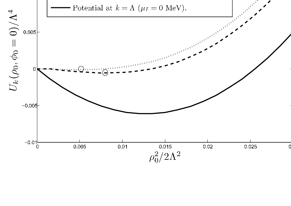
In Fig. 2 we show the real part ³³ 3 Note that the effective potential in the broken phase has an imaginary part to the left of the minimum. of the scaled effective potential as function of $\phi_{0}^{2}/2\Lambda^{2}$ in the chiral limit and for $T=0$ at $\mu_{I}=0$ and $\mu_{I}=30$ MeV.

We use the experimental value $f_{\pi}=93$ MeV and $m_{\sigma}=400$ MeV to tune the bare parameters in this case. We chose the cutoff $\Lambda^{2}=5m_{\sigma}^{2}$. This gives the values $m^{2}_{\Lambda}=-0.96\Lambda^{2}$ and $g_{\Lambda}^{2}=37.56$. We find that the inclusion of a finite chemical potential has the effect of increasing the $\rho_{0}$ value for which $U_{k}(\phi)$ takes its minimum. We also see that including the quantum fluctuations from the bosons reduces the amount of symmetry breaking. For fermions, the effect is opposite due a sign change of the vacuum term in the flow equation. Moreover, if the symmetry is restored for some values of $T$ and $\mu_{I}$ at $k=0$, there exists a scale $k=k_{\rm SSB}$ such $\Gamma[\phi]_{k}$ still displays symmetry breaking when $k>k_{\rm SSB}$.

In Fig. 3, we show the chiral condensate and pion condensate as function of $\mu_{I}$ at zero temperature. We have used the parameters $f_{\pi}=93$ MeV, $m_{\sigma}=600$ MeV, $m_{\pi}=140$ MeV, and $\Lambda=600$ MeV. The solid line is the local-potential approximation with $N=2$, the dashed line is the large-$N$ result, and the dotted line is the mean-field result. In the chiral limit the charged pion condensate is the only condensate present at nonzero chemical potential when $T=0$. If we go to the physical point however, we see that a chiral condensate appears in the direction of $\phi_{0}$. For small chemical potentials, we find that the chiral condensate is the only existing condensate, that is, the minimum of $U_{k}(\phi)$ lies on the $\phi_{0}$-axis and no charged pion condensation takes place. As we increase the chemical potential however, the minimum eventually moves away from the $\phi_{0}$-axis and a charged pion condensate is formed, i.e. the chiral condensate is (partly) rotated into a condensate of charged pions. At $T=0$ we find that this happens when the chemical potential is about the vacuum pion mass. This is in agreement with the results of e.g. [10, 12, 16, 17, 26] (but see the discussion below).

In Fig. 4, we plot the phase diagram as function of temperature and isospin chemical potential in the chiral limit (dashed line) and at the physical point (solid line). We use the same parameters as before. The phase diagram is in qualitative agreement with previous results [12, 16, 17, 26]. In particular, the phase transition to a condensate of pions is of second order and this is in accord with universality-class arguments. Note, however, that the critical chemical potential for $T=0$ and at the physical point is different from the pion mass $m_{\pi}$ and this is in disagreement with exact results. In fact, it can be shown that the critical chemical potential for Bose condensation at $T=0$ is equal to the mass of the condensing mode. Using the bare parameters we found at $T=\mu_{I}=0$, we see from Fig. 4 that we obtain a slightly different value for the critical chemical potential, namely $\mu_{I}^{c}=135$ MeV. The reason we do not get the pion mass is that we are working in the local-potential approximation, where wave-function renormalization is neglected. Recall that to include an isospin chemical potential we should let $\partial_{0}\Phi\rightarrow(\partial_{0}-\mu_{I})\Phi$, where we view the Lagrangian as a function of complex field variables. This term remains unrenormalized in the local-potential approximation and so the effective action is not gauge invariant under the transformations (5) - (6). This is in contrast to the full quantum effective action at $T=0$ [55].

A simple solution to this problem is to first solve the flow equation for the effective potential $U_{k}(\phi)$ in the absence of the isospin chemical potential and then gauge the effective action in the local-potential approximation by the substitution $\partial_{0}\Phi\rightarrow(\partial_{0}-\mu_{I})\Phi$. The effective potential at scale $k$ may then be written as

where $\tilde{U}_{k}(\phi)$ denotes the $O(4)$-symmetric potential, i.e. the potential satisfying Eq. (9) with $\mu_{I}=0$, that is Eq. (38) in the Appendix. We call this the $O(4)$-approximation. In order to get a charged pion condensate at $k=0$, one needs a negative partial derivative in the $\rho_{0}$ direction at the minimum of $U_{k}(\phi)$. When $\mu_{I}$ is just large enough for this to happen, we obtain

Using the $O(4)$-invariance of $\tilde{U}_{k}(\phi)$ and combining Eq. (15) with Eq. (12), this yields a critical chemical potential

While the effective potential $U_{k}(\phi)$ defined by Eq. (14) is in agreement with exact results, its dependence on the isospin chemical potential is of course trivial.

The large-$N$ limit provides us with another flow equation for $U_{k}(\phi)$ which is independent of the chemical potential. It is given by Eq. (39) in the Appendix:

Thus using the same arguments as above, we obtain the critical chemical potential for pion condensation which is equal to the pion mass.

In Fig. 5, we show the phase diagram obtained by solving the flow equation for $U_{k}(\phi)$ in the $O(4)$-approximation and in the large-$N$ limit. For comparison, we also show the phase diagram obtained by solving Eq. (9) and was shown in Fig. 4 albeit with a different cutoff $\Lambda$. In this plot, we used $\Lambda=1500$ MeV (Note that the dotted lines are from Fig. 4 with $\Lambda=600$ MeV). We would like to point out that both the $O(4)$ approximation and the large-$N$ approximation yield a second-order transition and adding the term $-\mbox{$1\over 2$}\mu_{I}\rho_{0}^{2}$ does not change this. Hence all three approximations predict the correct order of the transition.

In closing, we remark that it would be interesting to include the effects of wavefunction renormalization. This would lead to a set of coupled equations for $Z_{k}^{i}$ and $U_{k}(\phi)$. Hopefully it would close the gap between the value $\mu_{I}^{c}=135$ MeV obtained in this work and the exact result $\mu_{I}^{c}=m_{\pi}=140$ MeV and so perhaps provide a practical solution to the problems of the local-potential approximation. Similarly, it would be interesting to apply the method to the chiral quark model. Since this model has quark degrees of freedom, one can simultaneously study the effects of a baryon and an isospin chemical potential. In particular, one can investigate the BEC-BCS transition as one increases $\mu_{I}$. For small values of $\mu_{I}$, but larger than $m_{\pi}$, there is a condensate of pions. For asymptotically large values of $\mu_{I}$, and therefore large densities, the system is weakly coupled due to asymptotic freedom. In that case, the weak attraction gives rise to Cooper pairs and a BCS state. The order parameter has the same quantum numbers as the BEC state and so the transition is a crossover [1].

The BEC-BCS transition has been discussed at length in the functional renormalization group framework for ultracold atomic gases [56, 57, 58]. The crossover in these nonrelativistic systems is realized by changing the $s$-wave scattering length. This is done by varying an external magnetic field $B$ and exploiting the existence of a Feshbach resonance at $B_{0}=834$ Gauss. In this way one can basically change the coupling constant from minus infinity to plus infinity. A BEC state is obtained for positive scattering lengths and a BCS state for negative scattering lengths, i. e. on each side of the resonance.

The authors would like to thank Tomas Brauner, Holger Gies, and Michael Strickland for useful discussions.

In this Appendix, we derive the flow equation (9). The starting point is the exact flow equation (1) [31]

The effective potential $U_{k}(\phi)$ is defined by evaluating the effective action $\Gamma_{k}[\phi]$ for space-time independent values of the fields, i. e.

where $VT$ is the spacetime volume of the system and $\phi_{\rm uni}$ is constant. Taking the derivative of Eq. (19) with respect to $k$, we obtain the RG-equation for the effective potential

In the remainder we drop the subscript ${\rm uni}$. With $\Gamma_{k}[\phi]$ given as in Eq. (18), we find the Fourier transform of $\Gamma^{(2)}_{k}[\phi]$ to be

where $d$ denotes the spacetime dimension and $i,j$ are the indices of the propagator. Note that by the presence of the chemical potential, $\Gamma^{(2)}_{k,i,j,q,q^{\prime}}$ is not a diagonal matrix. Also note that we cannot rotate the field vector $\phi=(\phi_{1},..,\phi_{2N})$ to point in one specific direction as we do not have $O(2N)$ symmetry. This has been explicitly broken to a $O(2)\times O(2N-2)$ by the isospin chemical potential $\mu_{I}$. The best we can do is to write $\phi=(\phi_{0},0,\rho_{0},,0,..,0)$ to incorporate both a chiral condensate and a charged pion condensate. This will also give rise to off-diagonal entries in the matrix. We now set $N=2$ in order to simplify the derivation. Returning to a general $N$ is straightforward.

We may assume, because of the $O(2)\times O(2)$ symmetry, that $U_{k}(\phi)=U_{k}(\rho_{1},\rho_{2})$ where

If we denote the fields by double indices $\phi=(\phi_{11},\phi_{12},\phi_{21},\phi_{22})$, we can derive the identity

The Fourier transform of $R_{k}(x-y)$ is $(2\pi)^{d}\delta(q+q^{\prime})R_{k}(q)=R_{k,q,q^{\prime}}$. If we add $\delta_{ij}R_{k,q,q^{\prime}}$ to $\Gamma^{(2)}_{k,i,j,q,q^{\prime}}$, we obtain the matrix

where $F_{k}(q)=q^{2}+R_{k}(q)$. Using the fact that the inverse in Fourier space satisfies

we may invert $\big[\Gamma^{(2)}_{k}+R_{k}\big]_{q,q^{\prime}}$ to obtain the full $k$-dependent propagator. This may then be inserted into Eq. (20) in order to obtain the RG equation for the effective potential. Going to imaginary time we replace the integral over $q_{0}$ by a Matsubara sum $T\sum_{n}$. This yields

where now $q^{2}=\omega_{n}^{2}+\mathbf{q}^{2}$ and $\omega_{n}=2\pi nT$ denotes the Matsubara frequencies. The difference between this and arbitrary $N$ is that there would be $2N-3$ propagators of the form of the last term in the above expression.

Performing the integral over $\mathbf{q}$ and returning to arbitrary $N$, we may simplify this by writing

where we have defined

The denominator $D(\omega_{n}^{2})$ is a third-degree polynomial in $\omega_{n}^{2}$. Writing out its roots $P_{i}$ would take several pages. However, they can in principle be found, so we may for the sake of argument assume that we have found them. If we denote by $R_{i}$ the residue of the three poles $P_{i}$ of $1/D(\omega_{n}^{2})$, we may write

Summing over the Matsubara frequencies yields

Finding the poles $P_{i}$ and the residues $R_{i}$ is done numerically, by use of the residue function in Matlab.

In the case of zero chemical potential there is only the possibility of a chiral condensate. The situation is again $O(2N)$ symmetric. Eq. (35) then reduces to

The equation thus obtained is

where $\omega_{1}=\sqrt{k^{2}+\partial_{1}U_{k}(\rho_{1})+2\rho_{1}\partial^{2}U_{k}(\rho_{1})}$ and $\omega_{2}=\sqrt{k^{2}+\partial_{1}U_{k}(\rho_{1})}$.

The large-$N$ limit of Eq. (36) is obtained by scaling the fields $\phi_{i}\rightarrow\sqrt{N}\phi_{i}$. This implies that $U_{k}\rightarrow NU_{k}$ on the left-hand side of Eq. (36). Letting $N\rightarrow\infty$, we obtain

Note that the flow equation (39) is independent of the isospin chemical potential.

References

- [1] D. T. Son and M. A. Stephanov, Phys. Rev. Lett. 86 (2001) 592.
- [2] J. B. Kogut, M. A. Stephanov, and D. Toublan, Phys. Lett. B 464 (1999) 183;J. B. Kogut, M. A. Stephanov, D. Toublan, J. J. M. Verbaarschot, and A. Zhitnitsky, Nucl. Phys. B 582 (2000) 477.
- [3] J. B. Kogut and D. K. Sinclair, Phys. Rev. D 64 (2001) 034508; ibid D 66 34505 (2002); ibid D 70 (2004) 094501.
- [4] S. Gupta, e-Print: arXiv:hep-lat/0202005.
- [5] P. de Forcrand, M. A. Stephanov, U. Wenger, PoS LAT2007 (2007) 237.
- [6] W. Detmold, M. J. Savage, A. Torok, S. R. Beane, T. C. Luu, K. Orginos, and A. Parreno, Phys. Rev. D 78, (2008) 014507.
- [7] S. R. Beane, W. Detmold, T. C. Luu, K. Orginos, M. J. Savage, and A. Torok, Phys. Rev. Lett. 100, (2008) 082004.
- [8] K. Splittorff, D. T. Son and M. Stephanov, Phys. Rev. D 64 (2001) 016003.
- [9] M. Loewe and C. Villavicencio, Phys. Rev. D 67 (2003) 074034; ibid D 70 (2004) 074005; ibid D 71 (2005) 094001.
- [10] A. Barducci, R. Casalbuoni, G. Pettini, and L. Ravagli, Phys. Lett. B 564 (2003) 217.
- [11] A. Jakovac, A. Patkos, Z. Szep, and P. Szepfalusy, Phys. Lett. B 582 (2004) 179.
- [12] T. Herpay and P. Kovacs, Phys. Rev. D 78 (2008) 116008.
- [13] M. Matsuzaki, Phys. Rev. D 82 (2010) 016005.
- [14] J. I. Kapusta, Phys. Rev. D 24 (1981) 426.
- [15] H. E. Haber and H. A. Weldon, Phys. Rev. D 25 (1982) 502.
- [16] L. He, M. Jin, and P. Zhuang, Phys. Rev. D 71 (2005) 116001.
- [17] J. O. Andersen, Phys. Rev. D 75 (2007) 065011.
- [18] J. O. Andersen and T. Brauner, Phys. Rev. D 78 (2008) 014030.
- [19] S. Shu and J.-R. Li, J.Phys. G 34 (2007) 2727.
- [20] Z. Zhang and Y.-X. Liu, Phys. Rev. C 75 (2007) 035201.
- [21] A. Barducci, R. Casalbuoni, G. Pettini, and L. Ravagli, Phys. Rev. D 69 (2004) 096004.
- [22] D. Ebert and K.G. Klimenko, J. Phys. G Nucl. Part. Phys. 32 (2006) 599.
- [23] D. Ebert and K.G. Klimenko, Eur. Phys. J. C 46 (2006) 771.
- [24] S. Lawley, W. Bentz, and A. W. Thomas, Phys. Lett. B 632 (2006) 495.
- [25] X. Hao and P. Zhuang, Phys.Lett. B 652 (2007) 275.
- [26] J. O. Andersen and L. T. Kyllingstad, J. Phys. G 37 (2010) 015003.
- [27] H. Abuki, R. Anglani, M. Pellicoro, and M. Ruggieri, Phys. Rev. D 79 (2009) 034032.
- [28] Z. Zhang and Yu-xin Liu, Phys. Rev. C 75, (2007) 064910.
- [29] H. Abuki, M. Ciminale, R. Gatto, N.D. Ippolito, G. Nardulli, and M. Ruggieri, Phys. Rev. D 78 (2008) 014002; M. Ruggieri, Prog. Theor. Phys. Suppl. 174, (2008) 60.
- [30] G.-F Sun, L. He, and P. Zhuang, Phys. Rev. D 75 (2007) 096004.
- [31] C. Wetterich, Nucl. Phys. B. 352 (1991) 529.
- [32] D. F. Litim and J. M. Pawlowski, Presented at Workshop on the Exact Renormalization Group, Faro, Portugal, 10-12 Sep 1998. Published in Faro 1998, The exact renormalization group, 168-185, e-Print: arXiv:hep-th/9901063.
- [33] J. Polonyi, Central Eur. J. Phys. 1 (2003) 1.
- [34] J. Berges, N. Tetradis, and C. Wetterich, Phys. Rep. 363 (2002) 223.
- [35] H. Gies, ECT School on Renormalization Group and Effective Field Theory Approaches to Many-Body Systems, Trento, Italy, 27 Feb-10 Mar 2006, e-Print: arXiv:hep-ph/0611146.
- [36] J. M. Pawlowski, Annals Phys. 322 (2007) 2831.
- [37] B.-J. Schaefer and J. Wambach, Phys. Part. Nucl. 39 (2008) 1025.
- [38] P. Kopietz, L. Bartosch, and F. Schütz, Introduction to the Functional Renormalization group, Springer-Verlag, Berlin Heidelberg, 2010.
- [39] O. J. Rosten, e-Print: arXiv:1003.1366 [hep-th].
- [40] E. E. Svanes, Masters’ thesis NTNU 2010: The Non-Perturbative Rnormalization Group with Applications, http://www.nt.ntnu.no/users/jensoa/svanes.pdf.
- [41] T. R. Morris and M. D. Turner, Nucl. Phys. B 509 (1998) 637.
- [42] J. Berges, D.-U. Jungnickel, and C. Wetterich, Eur. Phys. J. C 13 (2000) 323.
- [43] B.-J.Schaefer and J. Wambach, Nucl. Phys. A 757 (2005) 479.
- [44] J. Braun, Phys. Rev. D 81 (2010) 016008.
- [45] T. K. Herbst, J. M. Pawlowski, B.-J. Schaefer, Phys. Lett. B 696 (2011) 58.
- [46] J.-P. Blaizot, A. Ipp, and N. Wschebor, Nucl. Phys. A 849 (2011) 165.
- [47] J.-P. Blaizot, A. Ipp, R. Mendez-Galain, N. Wschebor, Nucl. Phys. A 784 (2007) 376.
- [48] F. Benitez, J.-P. Blaizot, H. Chate, B. Delamotte, Phys. Rev. E 80 (2009) 030103.
- [49] R. D. Ball, P. E. Haagensen, J. I. Latorre, E. Moreno, Phys. Lett. B 347, 80 (1995).
- [50] J. O. Andersen and M. Strickland, Phys. Rev. A 60 (1999) 1442.
- [51] D. Litim, Phys. Rev. D 64 (2001) 105007.
- [52] L. Canet, B. Delamotte, D. Mouhanna, and J. Vidal, Phys. Rev. D 67 (2003) 065004.
- [53] D. F. Litim and J. M. Pawlowski, JHEP 026, (2006) 11.
- [54] C. Vafa and E. Witten, Nucl. Phys. B 234 (1984) 173.
- [55] D.T. Son, e-Print: arXiv:hep-ph/0204199.
- [56] S. Floerchinger, PhD thesis, University of Heidelberg, (2009), e-Print: arXiv:0909.0416 [cond-mat.quant-gas].
- [57] S. Diehl, S. Floerchinger, H. Gies, J. M. Pawlowski, and C. Wetterich, Ann. Phys. 522, (2010) 615.
- [58] M. M. Scherer, S. Floerchinger, and H. Gies, http://arxiv.org/abs/1010.2890.