Categorification of a frieze pattern determinantThanks: This work was supported by the Engineering and Physical Sciences Research Council [grant numbers EP/S35387/01 and EP/G007497/1] and the Forschungsinstitut für Mathematik (FIM) at the ETH, Zürich. Karin Baur was supported by the Swiss National Science Foundation (grant PP0022-114794).

Consider a generic $2\times n$ matrix, i.e. a matrix

whose entries are indeterminates. For a choice of two columns of $X$, $1\leq i,j\leq n$, let

be the corresponding minor of $X$ (so $\Delta_{ii}=0$). Let $A$ be the symmetric matrix with entries $A_{ij}$ given by:

Our main result is the following.

Our motivation comes from a result of Broline, Crowe and Isaacs [BCI] concerning frieze patterns of integers. Theorem 1.1 can be regarded as a generalisation of this result, which we now describe.

Frieze patterns of integers in the plane were considered in [Cox, CoCox1, CoCox2] by Conway and Coxeter. Such a frieze pattern consists of a finite number of infinite rows of integers, with each row interlacing its neighbouring rows, and satisfies the unimodular rule, which states that for every four adjacent numbers forming a square:

the relation $ad-bc=1$ is satisfied. The entries in the first and last row are zero; the entries in the second and penultimate rows are $1$, and all other entries should be positive.

Fix an integer $n\geq 3$. A frieze pattern is said to be of order $n$ if it has $n+1$ rows. We fix a regular $n$-sided polygon $\PP_{n}$, with vertices $1,2,\ldots,n$ numbered in cyclic order, arranged clockwise around the boundary (we work with the vertices modulo $n$, with representatives in $\{1,2,\ldots,n\}$). In [CoCox1, CoCox2] it is shown that a frieze pattern can be obtained from a triangulation $\pi$ of $\PP_{n}$ in the following way. For each pair of integers $i,j\in\{1,2,\ldots,n\}$, define an integer $m_{ij}$ as follows. Set $m_{ii}=0$ and $m_{i,i+1}=1$ for all $i$. Then let $m_{i-1,i+1}$ be the number of triangles in $\pi$ incident with vertex $i$. Define $m_{ij}$ for all $i<j$ inductively using the formula

Then set $m_{ji}=m_{ij}$ for all $i<j$. The numbers $m_{ij}$ are all positive integers and, when arranged as in Figure 1, form a frieze pattern. Furthermore, every frieze pattern of order $n$ arises from a triangulation of $\PP_{n}$ in this way.

Note that the entries lying in a triangle below $m_{1,n}$ form a fundamental domain for a glide reflection preserving the pattern. This fundamental domain is indicated by a dashed line triangle (together with its shift to the right).

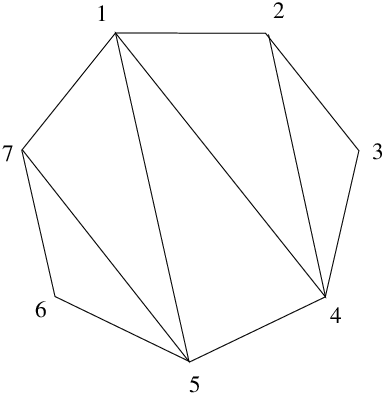
For example, the frieze pattern corresponding to the triangulation in Figure 2 is shown in Figure 3. The middle triangle indicates the fundamental domain mentioned above; its images under the glide reflection and its inverse are also displayed.

The result of Broline, Crowe and Isaacs can be stated as follows.

For the example in Figure 2, we have

which has determinant $-(-2)^{5}=32$. In addition, a geometric interpretation of all of the entries in the frieze pattern in terms of $\pi$ is given in [BCI].

We note that frieze patterns of integers of various kinds have been studied recently; see, for example [ARS, BM2, BR, G, KS, M-G, MOT, P].

A connection between cluster algebras and frieze patterns was established in the article [CaCh], which showed that the frieze patterns above can be obtained from cluster algebras of type $A$.

The homogeneous coordinate ring of the Grassmannian of $2$-planes in a $n$-dimensional vector space is a cluster algebra of type $A_{n-3}$ [FZ2, 12.6] (see also [FZ1, §1]). The cluster variables are in bijection with the diagonals of $\PP_{n}$. If $i,j$ are the end-points of such a diagonal, we write $u_{ij}$ for the corresponding cluster variable (so $u_{ij}=u_{ji}$). It has stable variables $u_{ij}$ where $i,j$ are the end-points of a boundary edge. We set $u_{ii}=0$ for all $i$ and $u_{ij}=u_{ji}$ for $i>j$.

Via the above bijection, the clusters are in bijection with the triangulations of $\PP_{n}$. We fix such a triangulation $\pi$ and corresponding cluster. By the Laurent Phenomenon [FZ1, 3.1], each cluster variable can be written as a Laurent polynomial in the elements of the cluster with the coefficients of the polynomial given by polynomials in the stable variables.

When the variables in the cluster and the stable variables are specialised to $1$, the resulting integers, when arranged correctly, produce the corresponding frieze pattern.

Theorem 1.1 can be reinterpreted in terms of this cluster algebra as follows. In this way we see that it is in fact a generalisation of Theorem 1.2.

We go on to show that this result can be given a categorical interpretation in terms of the root category of type $A_{n-1}$. By interpreting this category as a category of oriented edges between vertices of $\PP_{n}$ (using methods similar to those in [CaChS]) we show that the above determinant can be reinterpreted as a sum over configurations of indecomposable objects in the root category. Each configuration is a maximal collection of indecomposable objects such that no object lies in the frame of the other (see Section 7 for the definition of frame) which is also of maximal cardinality.

In this section, we prove our main result:

Note that the identity in Theorem 2.1 can be restated as:

since $A_{n1}=\Delta_{1n}=-\Delta_{n1}$.

We consider a cluster algebra $\mathcal{A}$ of type $A_{n-3}$ associated to $\PP_{n}$, defined over the complex numbers. This cluster algebra appears in [FZ1, §1] and is described in detail in [FZ3, 12.2]; see alternatively [P, 3.2] (using a perfect matching model for frieze patterns due to Gabriel Carroll and Gregory Price; see [loc. cit.] for details).

Let $\pi$ be a triangulation of $\PP_{n}$ and let $\mathbb{F}$ be the field of rational functions in the variables $u_{ij}$ where $i,j$ are the end-points of a diagonal in $\pi$ or a boundary edge of $\PP_{n}$ (regarding $u_{ij}$ and $u_{ji}$ as equal). Define elements $u_{ij}\in\mathbb{F}$, for $i,j$ the end-points of an arbitrary diagonal of $\PP_{n}$, inductively as follows (again with $u_{ij}=u_{ji}$). If $i,j,k,l$ are vertices of $\PP_{n}$, arranged clockwise around the boundary, and $u_{ij},u_{jk},u_{kl},u_{li}$ and $u_{ik}$ are defined but $u_{jl}$ is not, define $u_{jl}$ by the following exchange relation:

It turns out that the elements $u_{ij}$ are well-defined. The cluster algebra $\mathcal{A}$ is the $\mathbb{C}$-subalgebra of $\mathbb{F}$ generated by the $u_{ij}$ for $i,j$ the end-points of any diagonal or boundary edge of $\PP_{n}$. The generators corresponding to diagonals are known as cluster variables and those corresponding to boundary edges are known as stable variables. For $n=3$ there are no cluster variables, only stable variables. The exchange relation (6) holds for any choice of $i,j,k,l$ arranged clockwise around the boundary of $\PP_{n}$.

The diagonals in a triangulation of $\PP_{n}$ determine a corresponding set of cluster variables of $\mathcal{A}$ known as a cluster. The cluster corresponding to $\pi$ is the initial cluster. By [FZ1, 3.1], the cluster variables can be written as Laurent polynomials in any fixed cluster, with coefficients given by polynomials in the stable variables.

The cluster algebra $\mathcal{A}$ is independent (up to isomorphism) of the choice of $\pi$. In fact, it is isomorphic to the homogeneous coordinate ring $\mathbb{C}[Gr_{2}(n)]$ of the Grassmannian of $2$-dimensional subspaces of an $n$-dimensional vector space; see [FZ2, 12.6]. Such a subspace can be described by a $2\times n$ matrix, with rows given by a choice of spanning vectors, and the $2\times 2$ minors of the matrix give homogeneous coordinates on the Grassmannian.

The homogeneous coordinate ring is generated by these minors, subject to the Plücker relations, and under the isomorphism, $u_{ij}$, for $i<j$, maps to the minor associated to columns $i$ and $j$ of the matrix. The exchange relations above map to the Plücker relations.

Fix a triangulation $\pi$ of $\PP_{n}$. Setting $u_{ii}=0$ for all $i$, we consider the symmetric matrix $U(\pi)=(u_{ij})$, where the $u_{ij}$ are regarded as Laurent polynomials in the $u_{ij}$ for $i,j$ the end-points of an edge in $\pi$ with coefficients given by polynomials in the stable variables.

We note the following:

Caldero-Chapoton prove this by first showing that, for each $i$, $u_{i-1,i+1}$ specialises to the number of triangles in $\pi$ incident with vertex $i$, which coincides with $m_{i-1,i+1}$ in the above definition. The result then follows from a comparison of formulas (1) and (6).

We can now restate Theorem 2.1 in this context. The proof of this version is the same, using the exchange relations (6) (and noting equation (5)).

We have thus interpreted Theorem 2.1 as a generalisation of Theorem 1.2.

Here we give an example of the result in the previous section. Let $\pi$ be the triangulation of a pentagon shown in Figure 5.

Then the corresponding matrix is given by:

where

By Theorem 3.2, we have that

Let $n\geq 3$ be an integer and let $Q$ be a quiver of type $A_{n-1}$. Let $k$ be an algebraically closed field. Let $D^{b}(kQ)$ denote the bounded derived category of modules over $kQ$, with shift functor $[1]$. Let $\mathcal{R}_{n}=D^{b}(kQ)/[2]$ denote the quotient of $D^{b}(kQ)$ by the square $[2]$ of the shift. In this section we shall exhibit a geometric construction of this category (along the lines of [CaChS]). We remark that this category is sometimes referred to as the root category (of type $A$) since its objects can be put into one-to-one correspondence with the roots in the corresponding root system (by Gabriel’s Theorem). It was considered in [H1].

We now consider oriented edges between vertices of $\PP_{n}$, denoting the edge oriented from $i$ to $j$ by $[i,j]$, for any $1\leq i,j\leq n$ with $i\neq j$ (thus boundary edges are included).

Recall that a stable translation quiver is a pair $(\Gamma,\tau)$ where $\Gamma$ is a locally finite quiver and $\tau:\Gamma_{0}\rightarrow\Gamma_{0}$ is a bijection such that for any $X,Y\in\Gamma_{0}$, the number of arrows from $X$ to $Y$ is the same as the number of arrows from $\tau(Y)$ to $X$.

Let $\Gamma=\Gamma(n)$ be the quiver defined as follows. The set of vertices, $\Gamma_{0}$, is the set of all possible oriented edges between distinct vertices of $\PP_{n}$ as above. The arrows, $\Gamma_{1}$, are of the form $[i,j]\rightarrow[i,j+1]$ and $[i,j]\rightarrow[i+1,j]$ (where $j+1$ is interpreted as $1$ if $j=n+1$ and similarly for $i+1$), whenever $[i,j]$ and $[i,j+1]$ (respectively, $[i,j]$ and $[i+1,j]$) are vertices of $\Gamma$. Thus an arrow comes from rotating an oriented edge clockwise about one of its end-points so that the other end-point moves to an adjacent vertex on the boundary of $\PP_{n}$.

Let $\tau$ be the automorphism of $\Gamma$ obtained by rotating $\PP_{n}$ through $2\pi/n$ anticlockwise; thus $\tau([i,j])=[i-1,j-1]$.

The proof is as in [BM1, 2.2]: note that this proof also works in the oriented case we have here.

By [PX, 2.3] (see also [K, 9.9]), $\mathcal{R}_{n}$ is a triangulated category, and, by [BMRRT, 1.3], it has Auslander-Reiten triangles and its Auslander-Reiten quiver, $\Gamma(\mathcal{R}_{n})$ is the quotient of the Auslander-Reiten quiver of $D^{b}(kQ)$ by the automorphism induced by $[2]$. We have the following:

We note that, as for the cluster category (see [BMRRT, §1]), the category $\mathcal{R}_{n}$ is standard. We thus have the following corollary of Proposition 5.3, giving a geometric realisation of $\mathcal{R}_{n}$.

We shall identify indecomposable objects in $\mathcal{R}_{n}$, up to isomorphism, with the corresponding oriented edges between vertices of $\PP_{n}$, in the sequel, and we shall freely switch between objects and oriented edges between vertices in $\PP_{n}$.

In this section we indicate how the dimensions of $\Ext^{1}$-groups between indecomposable objects of $\mathcal{R}_{n}$ can be read off from the geometric model. We fix $i,j$ with $1\leq i,j\leq n$, $i\neq j$, and consider the corresponding indecomposable object $[i,j]$.

Consider the two rectangles $R_{B}=R_{B}(i,j)$, with corners $[j,i]$, $[j,j-1]$, $[i-1,j-1]$ and $[i-1,i]$, and $R_{F}=R_{F}(i,j)$, with corners $[i+1,j+1]$, $[i+1,i]$, $[j,i]$ and $[j,j+1]$, in $\mathcal{R}_{n}$.

Note that the Auslander-Reiten formula holds in $D^{b}(kQ)$. This states that, for two indecomposable objects $X,Y$ in $D^{b}(kQ)$,

where $D=\Hom_{k}(-,k)$. This passes down to the root category $\mathcal{R}_{n}$ and it follows that the dimensions of $\Ext^{1}_{\mathcal{R}_{n}}(X,Y)$ and $\Hom_{\mathcal{R}_{n}}(Y,\tau X)$ coincide for any two indecomposable objects $X,Y$ in $\mathcal{R}_{n}$.

Using [B] or the mesh relations and the Auslander-Reiten formula in $\mathcal{R}_{n}$ directly, we see that:

As an example, we show in Figure 8 (by underlining) those indecomposable objects $Y$ such that $\Ext^{1}_{\mathcal{R}_{5}}([3,1],Y)\neq 0$ for the case $n=5$, and (by overlining) those indecomposable objects $X$ such that $\Ext^{1}_{\mathcal{R}_{5}}(X,[3,1])\neq 0$. In each case the objects in question are written in bold font. Note that $[1,3]$ is the only object satisfying both conditions.

Let $X,Y$ be two indecomposable objects of $\mathcal{R}_{n}$, regarded as oriented edges between vertices of $\PP_{n}$. Then $X$ and $Y$ may cross each other in two different ways. If the tangents to $X,Y$ (in that order) form a pair of axes corresponding to the usual orientation on $\mathbb{R}^{2}$ we say that the crossing of $X$ and $Y$ is positive, otherwise negative. See Figure 7.

Lemma 6.1 can be reinterpreted geometrically as follows.

As an example, consider the objects $Y$ such that $\Ext^{1}_{\mathcal{R}_{5}}([3,1],Y)\not=0$, displayed in Figure 8 (by underlining). Note that the crossing of $[3,1]$ with $[2,5]$ or with $[2,4]$ is positive; both $[1,4]$ and $[1,5]$ start at the terminal vertex of $[3,1]$ and lie to its left; $[2,3]$ has terminal vertex coinciding with the initial vertex of $[3,1]$ and lies to its right, and $[1,3]$ is the reverse of $[3,1]$.

In this section we consider starting and ending frames of indecomposable objects in $\mathcal{R}_{n}$ (following [BMRRT, 8.4]). Let $\ind(\mathcal{R}_{n})$ denote the set of (isomorphism classes of) indecomposable objects of $\mathcal{R}_{n}$. Let $X$ be an indecomposable object in $\mathcal{R}_{n}$. Then the starting frame $S(X)$ of $X$ is the set

The ending frame $E(X)$ of $X$ is the set

We define the frame $F(X)$ of $X$ to be the union:

The following can be checked by direct calculation or using Proposition 6.2 and the Auslander-Reiten formula.

We also note that, if $\overline{X}$ denotes the reverse of $X$, then

and

Fix again a triangulation $\pi$ of $\PP_{n}$. For $1\leq i,j\leq n$ with $i\neq j$, we associate the indecomposable object $[i,j]$ (or oriented edge) with the $i,j$ position in the $n\times n$ matrix $U(\pi)$ considered in Section 1. The indecomposable $kQ$-modules (with $i<j$) correspond to the part of $U(\pi)$ above the leading diagonal and their shifts (with $i>j$) correspond to the part of $U(\pi)$ below the leading diagonal.

Reinterpreting Proposition 7.1 in these terms, we obtain:

Define a frame-free configuration of $\mathcal{R}_{n}$ to be a maximal collection $C$ of (isomorphism classes of) indecomposable objects of $\ind\mathcal{R}_{n}$ such that $Y\not\in F(X)$ for all $X,Y$ in $C$. Thus frame-free configurations of $\mathcal{R}_{n}$ correspond to maximal collections of positions in $U(\pi)$ which do not lie in the same row or column as each other and contain no diagonal entries.

Given a fixed-point free permutation, $\sigma$ (sometimes known as a derangement), let $C(\sigma)$ be the set of objects $[i,\sigma(i)]$ for $1\leq i\leq n$. Since $\sigma$ is fixed-point free, it follows from Proposition 7.1(c) that $C(\sigma)$ is a frame-free configuration; it has cardinality $n$. It is clear that this gives a bijection between fixed-point free permutations and frame-free configurations of cardinality $n$.

Thus, as a collection of oriented edges between vertices of $\PP_{n}$, a frame-free configuration in $\mathcal{R}_{n}$ of cardinality $n$ is a union of oriented cycles (with no cycles of cardinality $1$).

Similarly, a permutation $\sigma$ with one fixed point, $p$, say, corresponds to a configuration of cardinality $n-1$ consisting of the objects $[i,\sigma(i)]$ for $i\neq p$. This gives a bijection between the permutations with a single fixed point and the frame-free configurations of cardinality $n-1$.

The number of permutations with a given number of fixed points is well-known (see e.g. [S, A008290]). We thus have the following:

Thus the number of frame-free configurations in $\mathcal{R}_{n}$ of cardinality $n$ for $n=2,3,\ldots$, is $1,2,9,44,265,1854$ (see [S, A000166]) and the number of frame-free configurations in $\mathcal{R}_{n}$ of cardinality $n-1$ is $0,3,8,45,264,1855$ (see [S, A000240]). The $9$ frame-free configurations of $\mathcal{R}_{4}$ of cardinality $4$ are shown in Figure 9 as collections of vertices in the AR-quiver (filled in vertices indicate those indecomposable objects in the collection) and as collections of oriented arcs between vertices of a square.

We see that the frame-free configurations of $\mathcal{R}_{n}$ of cardinality $n$ correspond bijectively to the non-zero terms in the expansion

References

• [ARS] I. Assem, C. Reutenauer and D. Smith. Friezes. Adv. Math. 225 (2010), no. 6, 3134–3165.
• [BM1] K. Baur and R. J. Marsh. A geometric description of m-cluster categories. Trans. Amer. Math. Soc. 360 (2008), 5789-5803.
• [BM2] K. Baur and R. J. Marsh. Frieze patterns for punctured discs. J. Algebraic Combin. 30 (2009), no. 3, 349–379.
• [BR] F. Bergeron and C. Reutenauer, S​LkSL_{k}-Tilings of the Plane. Illinois J. Math. 54 (2010), no.1, 263–300.
• [B] K. Bongartz. Critical simply connected algebras. Manuscripta Math. 46 (1-3) (1984) 117–136.
• [BCI] D. Broline, D. W. Crowe and I. M. Isaacs. The geometry of frieze patterns. Geom. Ded. 3 (1974), 171–176.
• [BMRRT] A. B. Buan, R. Marsh, M. Reineke, I. Reiten and G. Todorov, Tilting theory and cluster combinatorics. Adv. Math. 204 (2006), no. 2, 572–618.
• [CaCh] P. Caldero and F. Chapoton. Cluster algebras as Hall algebras of quiver representations. Commentarii Mathematici Helvetici, 81, (2006), 595-616.
• [CaChS] P. Caldero, F. Chapoton and R. Schiffler. Quivers with relations arising from clusters (AnA_{n} case). Trans. Amer. Math. Soc. 358 (2006), no. 3, 1347–1364.
• [Cox] H. S. M. Coxeter. Frieze patterns. Acta Arith. XVIII (1971), 297–310.
• [CoCox1] J. H. Conway and H. S. M. Coxeter, Triangulated polygons and frieze patterns. Math. Gaz. 57 (1973), 87–94.
• [CoCox2] J. H. Conway and H. S. M. Coxeter, Triangulated polygons and frieze patterns. Math. Gaz. 57 (1973), 175–186.
• [FZ1] S. Fomin and A. Zelevinsky, Cluster algebras. I. Foundations. J. Amer. Math. Soc. 15 (2002), no. 2, 497–529.
• [FZ2] S. Fomin and A. Zelevinsky, Cluster algebras II: Finite type classification. Invent. Math. 154 (2003), no. 1, 63–121.
• [FZ3] S. Fomin and A. Zelevinsky. YY-systems and generalized associahedra. Ann. Math. 158 (2003), no. 3, 977–1018.
• [G] L. Guo. On tropical friezes associated with Dynkin diagrams. Preprint arXiv:1201.1805v2 [math.RT], 2012.
• [H1] D. Happel, Tilting sets on cylinders. Proc. London Math. Soc. (3) 51 (1985), no. 1, 21–55.
• [H2] D. Happel, Triangulated categories in the representation theory of finite-dimensional algebras. London Mathematical Society Lecture Note Series, 119. Cambridge University Press, Cambridge, 1988.
• [K] B. Keller, On triangulated orbit categories. Doc. Math. 10 (2005), 551–581.
• [KS] B. Keller and S. Scherotzke, Linear recurrence relations for cluster variables of affine quivers. Adv. Math. 228 (2011), no. 3, 1842–-1862.
• [M-G] S. Morier-Genoud, Arithmetics of 2-friezes. Preprint arXiv:1109.0917v2 [math.CO], 2011. To appear in J. Algebraic Combin.
• [MOT] S. Morier-Genoud, V. Ovsienko and S. Tabachnikov, 22-frieze patterns and the cluster structure of the space of polygons. Preprint arXiv:1008.3359v2 [math.AG], 2010. To appear in Annales de l’Institut Fourier.
• [PX] L. Peng and J. Xiao, Root categories and simple Lie algebras. J. Algebra 198 (1997), no. 1, 19–56.
• [P] J. Propp. The combinatorics of frieze patterns and Markoff numbers. Preprint arxiv:math.CO/0511633, November 2005.
• [S] N. J. A. Sloane, Ed. (2008), The On-Line Encyclopedia of Integer Sequences, published electronically at www.research.att.com/∼\simnjas/sequences/.