Intra- and Inter-Session Network Coding
in Wireless Networks Thanks: H. Seferoglu is with the Laboratory for Information and Decision Systems (LIDS), Massachusetts Institute of Technology. Email: hseferog@mit.edu. Mail: 77 Massachusetts Avenue, Room 32-D671, Cambridge, MA 02139.Thanks: A. Markopoulou is with the Electrical Engineering and Computer Science Department, University of California, Irvine. Email: athina@uci.edu. Mail: CalIT2 Bldg, Suite 4100, Irvine, CA 92697.Thanks: K. K. Ramakrishnan is with AT&T Labs Research. Email: kkrama@research.att.com. Mail: 180 Park Avenue, Building 103 Florham Park, NJ 07932.

Let $\mathcal{S}$ be the set of unicast flows between source-destination pairs in the network. Each flow $s\in\mathcal{S}$ is associated with a rate $x_{s}$ and a utility function $U_{s}(x_{s})$, which we assume to be a strictly concave function of $x_{s}$.

Packets from a source (e.g., $S_{1}$ in Fig. 1) traverse potentially multiple wireless hops before being received by the receiver (e.g., $R_{1}$). We consider a model for interference described in [22]: each node can either transmit or receive at the same time, and all transmissions in the range of the receiver are considered as interfering.

We use the following terminology for wireless. A hyperarc $(i,\mathcal{J})$ is a collection of links from node $i\in\mathcal{N}$ to a non-empty set of next-hop nodes $\mathcal{J}\subseteq\mathcal{N}$. A hypergraph $\mathcal{H}=(\mathcal{N},\mathcal{A})$ represents a wireless mesh network, where $\mathcal{N}$ is the set of nodes and $\mathcal{A}$ is the set of hyperarcs. For simplicity, $h=(i,\mathcal{J})$ denotes a hyperarc, $h(i)$ denotes node $i$ and $h(\mathcal{J})$ denotes the set of nodes in $\mathcal{J}$, i.e., $h(i)=i$ and $h(\mathcal{J})=\mathcal{J}$. We use these notations interchangeably in the rest of the paper. Each hyperarc $h$ is associated with a channel capacity $R_{h}$. Since $h$ is a set of links, $R_{h}$ is the minimum capacity of all the links in the hyperarc, i.e., $R_{h}=\min_{j\in h(J)}\{R_{i,j}\}$ s.t. $i\in\mathcal{N}$. In the example of node $I$ in Fig. 1, $h=(I,\{B_{2},A_{2}\})$ is one of the hyperarcs, and its capacity is $\min\{R_{\{I,B_{2}\}},R_{\{I,A_{2}\}}\}$.

Note that with both intra- and inter-session NC, it is possible to construct more than one code over a hyperarc $h$. Let $\mathcal{K}_{h}$ be the set of inter-session network codes over a hyperarc $h$. $\mathcal{S}_{k}\subseteq\mathcal{S}$ be the set of flows coded together using code $k\in\mathcal{K}_{h}$ and broadcast over $h$.²² 2 Note that we consider constructive inter-session NC, i.e., network codes $k\in\mathcal{K}_{i,\mathcal{J}}$ as well as $h=(i,\mathcal{J})$ is determined at each node with periodic control packet exchanges or estimated through routing table.

Given $\mathcal{H}$, we can construct the conflict graph $\mathcal{C}=(\mathcal{A},\mathcal{I})$, whose vertices are the hyperarcs of $\mathcal{H}$ and edges indicate interference between hyperarcs. A clique $\mathcal{C}_{q}\subseteq\mathcal{A}$ consists of several hyperarcs, at most one of which can transmit without interference, i.e., a transmission over a hyperarc interferes with transmissions over other hyperarcs in the same clique.

A flow $s$ may experience loss in two forms: loss $\rho_{h}^{s}$ over the direct transmission links; or loss $\rho_{h,k}^{s,s^{\prime}}$ of antidotes³³ 3 Following the poison-antidote terminology of [4], we call “antidotes” the packets of flows $s^{\prime}$ that are coded together with $s$, and thus are needed for the next hop of $s$ to be able to decode. E.g., in Fig.1, $a$ is the “antidote” that $B_{2}$ needs to overhear over link $A_{1}-B_{2}$, to decode $a+b$ and obtain $b$. on overhearing links. These two types of loss have different impact on network coded flows.

First, let us discuss loss on the direct links. A flow $s$ transmitted over hyperarc $h$ experiences loss with probability $\rho_{h}^{s}$. This probability is different per flow $s$, even if several flows are coded and transmitted over the same hyperarc $h$, because different flows are transmitted to different next hops, thus see different channels. For example, in Fig. 1, $\rho_{(I,\{B_{2},A_{2}\})}^{S_{1}}$ is equal to the loss probability over link $I-A_{2}$ and $\rho_{(I,\{B_{2},A_{2}\})}^{S_{2}}$ is equal to the loss probability over link $I-B_{2}$.

Second, let us discuss the effect of lost antidotes on the overhearing link. Consider that flow $s$ is combined with flow $s^{\prime}$ s.t. $s\neq s^{\prime}$, and that some packets of flow $s^{\prime}$ are lost on the overhearing link to the next hop of $s$. Then, coded packets cannot be decoded at the next hop and flow $s$ loses packets, with probability $\rho_{h,k}^{s,s^{\prime}}$. For example, in Fig. 1, packets from flow $S_{1}$ cannot be decoded (hence are lost) at node $A_{2}$ due to loss of antidotes from flow $S_{2}$ on the overhearing link $B_{1}-A_{2}$.

In our formulation and analysis, we assume that $\rho_{h}^{s}$ and $\rho_{h,k}^{s,s^{\prime}}$ are i.i.d. according to a uniform distribution. However, in our simulations, we consider a Rayleigh fading channel model. The loss probabilities are calculated at each intermediate node as explained later in this section.

Each flow $s\in\mathcal{S}$ follows a single path $\mathcal{P}_{s}\subseteq\mathcal{N}$ from the source to the destination, which is pre-determined by a routing protocol, e.g., OLSR or AODV, and given as input to our problem. Note that the nature of wireless networks is time varying, i.e., nodes join and leave the system dynamically. In such cases, the routing protocol actively determines new paths which are used as input to our problem. It is not critical that the paths remain fixed, neither from a theoretical nor from a practical point of view, as explained in the following sections. Also, note that several different hyperarcs may connect two consecutive nodes along the path. We define $H_{h,k}^{s}=1$ if $s$ is transmitted through hyperarc $h$ using network code $k\in\mathcal{K}_{h}$; and $H_{h,k}^{s}\!=\!0$, otherwise.

Consider the commonly used generation-based NC [23]: packets from flow $s\in\mathcal{S}$ are divided into generations (note that we use “generation” and “block” terms interchangeably), with size $G^{s}$. At the source $s$, packets within the same generation are linearly combined (assuming large enough field size) to generate $G^{s}$ network coded packets. Each intermediate node along the path of flow $s$ adds $P^{s}$ parity packets, depending on the loss rates of the links involved in this hop. At the next hop, it is sufficient to receive $G^{s}$ out of $G^{s}+P^{s}$ packets. The same process is repeated at every intermediate node until the receiver receives $G^{s}$ error-free packets, which can then be decoded and be passed on to the application.

There are many ways to generate parities ($P^{s}$) in practice. We use generation based intra-session NC [23] for this purpose. Although one could use various coding techniques, such as Reed-Solomon or Fountain codes, using intra-session NC has several advantages. First, it has lower computational complexity. Second, in systems like COPE that already implement inter-session NC, it is natural to incrementally add intra-session NC functionality. Moreover, in this setting, hop-by-hop intra-session coding (in which redundant packets are generated at each hop) is clearly a better choice than end-to-end coding for dealing with loss. In terms of performance, hop-by-hop coding achieves higher end-to-end throughput (thanks to introducing less redundancy than end-to-end coding), without adding high complexity (and thus delay) to the intermediate nodes. Furthermore, in terms of system implementation, our hop-by-hop scheme requires minimal modifications on top of the inter-session NC, which is already implemented.

After an intermediate node has added redundancy ($P^{s}$) to flow $s$, it treats all ($G^{s}+P^{s}$) packets as indistinguishable parts of the same flow. Inter-session NC is applied on top of the already intra-coded flows, as a thin layer between MAC and IP (similar to COPE), shown in Fig. 2. We design two schemes, I²NC-state and I²NC-stateless, depending on the type of information that is needed to make network coding decisions. We define as state of a node the information about which exact packets have been overheard at that node.

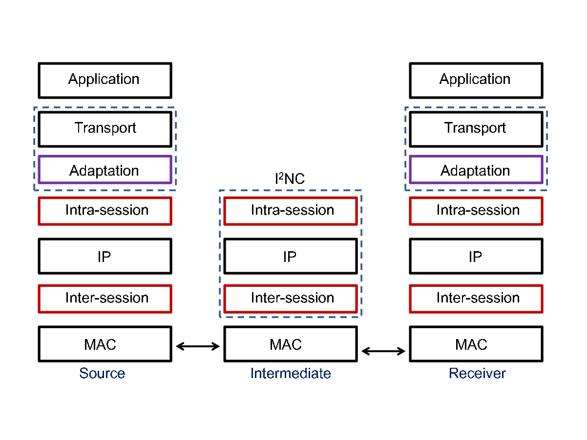
I²NC-state: First, we assume that intermediate nodes use COPE [2] for inter-session coding. Each node $i$ listens all transmissions in its neighborhood, stores the overheard packets in its decoding buffer, and periodically advertises the content of this buffer to its neighbors. When a node $i$ wants to transmit a packet, it checks or estimates the contents of the decoding buffer of its neighbors. If there is a coding opportunity, the node combines the relevant packets using simple coding operations (XOR) and broadcasts the combination to $\mathcal{J}$. The content of the decoding buffers needs to be exchanged, in order to make NC decisions, i.e., state synchronization is required.

I²NC-stateless: Second, we design an improved version of COPE, which no longer requires state synchronization. The key idea is to exploit the fact that the redundancy already introduced by intra-session coding makes all $G^{s}+P^{s}$ packets in a generation equally important.⁴⁴ 4 It no longer matters which exact packets a node has. As long as a node has any $G^{s}$ out of $G^{s}+P^{s}$, it can decode with high probability. As long as it knows the percentage of received packets it can make coding decisions. In this improved scheme, each node $i$ still listens to all transmissions in its neighborhood and stores the overheard packets.⁵⁵ 5 Note that when inter-session network coded packets are overheard, they are not stored in the “decoding buffer”, but discarded. The node periodically advertises the loss rate for each received and overheard flow, which is then provided as input to the intra-session NC module to determine the amount of redundancy needed. In particular, the loss rates are calculated at each intermediate node as one minus the ratio of correctly received packets over all the packets in a generation. Also, the loss rate over overhearing links is calculated as effective loss rate. E.g., in Fig. 1, the loss rate at node $A_{2}$ is calculated as follows. If $G^{S_{1}}+P^{S_{1}}$ packets are sent by $B_{1}$ and at least $G^{S_{1}}$ packets are received at $A_{2}$, then the loss rate is set to 0. If $G^{S_{1}}-u$ packets are received by $A_{2}$ such that $u\leq G^{S_{1}}$, then the loss rate is set to $u/G^{S_{1}}$. The loss rates calculated for each generation are advertised to other nodes in the neighborhood. Then, each node calculates its loss probabilities ($\rho_{h}^{s}$ and $\rho_{h,k}^{s,s^{\prime}}$) as weighted average of the loss rates it has received.

In summary, there is a synergy between intra- and inter-session NC. Intra-session makes the process sequence agnostic, which allows inter-session coding to operate using only information about the loss rates, not about the identity of the packets. The loss rates can be used as input for tuning the amount of redundancy in intra-session NC. In terms of implementation, the two modules are separable: an intermediate node first performs intra-session, then inter-session NC.

Our objective is to maximize the total utility function by optimally choosing the flow rates $x_{s}$ at sources $s\in\mathcal{S}$, as well as the following variables at the intermediate nodes: the fraction $\alpha_{h,k}^{s}$ (or “traffic splitting” parameters, following the terminology of [24]) of flows inter-session coded using code $k\in\mathcal{K}_{h}$ over hyperarc $h$; and the percentage of time $\tau_{h,k}$ each hyperarc is used.

The first constraint is the capacity constraint for each flow $s\in\mathcal{S}_{k}$. It is well-known, [25], that NC allows flows that are coded together in code $k\in\mathcal{K}_{h}$, to coexist, i.e., each have rate up to the rate allocated to that code $k$. The right hand side, $R_{h}\tau_{h,k}$, is the capacity of hyperarc $h$; $\tau_{h,k}$ is the percentage of time hyperarc $h$ can be used for transmitting the $k$-th network code. $\tau_{h,k}$ is determined by scheduling in the third constraint, taking into account interference: all hyperarcs in a clique interfere and should time-share the medium. Therefore, the sum of the time allocated to all hyperarcs in a clique should be less than an over-provisioning factor, $\gamma\leq 1$. The second constraint is the flow conservation: at every node $i$ on the path $\mathcal{P}_{s}$ of source $s$, the sum of $\alpha_{h,k}^{s}$ over all network codes and hyperarcs should be equal to 1. Indeed, when a flow enters a particular node $i$, it can be transmitted to its next hop $j$ as part of different network coded and uncoded flows.

The first constraint is key to our work because it determines how to deal with loss on the direct ($\rho_{h}^{s}$) and overhearing ($\rho_{h,k}^{s,s^{\prime}}$) links and how large a fraction ($\alpha_{h,k}^{s}$) of flow rate ($x_{s}$) to code in the $k$-th code over hyperarc $h$. Let us discuss the left hand side in more detail.⁶⁶ 6 Note that our formulation has two novel aspects, compared to prior work, which allow us to better handle loss and parities. First, we allow for flows coded together to have different rates (in the first constraint in Eq. (1)). Second, we allow for loss rates of each link to be specified separately, even for links in the same hyperarc.

The first term refers to the direct link of flow $s$. $H_{h,k}^{s}\alpha_{h,k}^{s}x_{s}$ is the fraction of flow rate $x_{s}$ allocated to code $k$ and hyperarc $h$. It is scaled by $1-\rho_{h}^{s}$ to indicate that we use redundancy to protect against loss that flow $s$ experiences with probability $\rho_{h}^{s}$. $(H_{h,k}^{s}\alpha_{h,k}^{s}x_{s})/(1-\rho_{h}^{s})$ is the total rate of flow $s$, including data and redundancy.

The second term refers to loss on the overhearing links. $\sum_{s^{\prime}\in\mathcal{S}_{k}-\{s\}}H_{h,k}^{s^{\prime}}\alpha_{h,k}^{s^{\prime}}x_{s^{\prime}}\rho_{h,k}^{s,s^{\prime}}$ is the amount of redundancy (via intra-session coding) added by the intermediate node on flow(s) $s^{\prime}$ to protect flow $s$ against loss of antidote packets. These antidotes come from other flows ($s^{\prime}\in\mathcal{K}_{h}$) that are coded together with flow $s$, reach the next hop for flow $s$ through the overhearing links, and are needed to decode inter-session coded packets.

Example 1- continued. In Fig. 1, let us consider flow 2 from $B_{1}$ to $B_{2}$, as the flow of interest. The intermediate node $I$ adds redundancy to $S_{2}$ to protect against loss rate $\rho_{(I,\{B_{2},A_{2}\})}^{S_{2}}$ on the direct link $I-B_{2}$. It also adds redundancy to flow 1 to protect against loss rate $\rho_{(I,\{B_{2},A_{2}\})}^{S_{2},S_{1}}$ of antidotes coming to $B_{2}$ from flow 1 over the overhearing link $A_{1}-B_{2}$.

To solve Eq. (1) we follow a similar approach proposed in [36]. First, we relax the capacity constraint in Eq. (1), and we have the Lagrangian function:

where $q_{h,k}^{s}$ is the Lagrange multiplier, which can be interpreted as the queue size for $k$-th network code at hyperarc $h$ for flow $s$. We define $\rho_{h,k}^{s,s^{\prime}}=0$ if $s=s^{\prime},\forall s,s^{\prime}\in\mathcal{S}$ and we rewrite $\sum_{k\in\mathcal{K}_{h}}$ $\sum_{s\in S_{k}}$ as $\sum_{s\in\mathcal{S}}$ $\sum_{k\in K_{h}\mid s\in\mathcal{S}_{k}}$. The Lagrange function is $L(\boldsymbol{x},\boldsymbol{\alpha},\boldsymbol{\tau},\boldsymbol{q})=\sum_{s\in\mathcal{S}}(U_{s}(x_{s})-x_{s}\sum_{h\in\mathcal{A}}\sum_{k\in\mathcal{K}_{h}\mid s\in\mathcal{S}_{k}}H_{h,k}^{s}\alpha_{h,k}^{s}((q_{h,k}^{s})$ $/(1-\rho_{h}^{s})+\sum_{s^{\prime}\in\mathcal{S}_{k}}q_{h,k}^{s^{\prime}}\rho_{h,k}^{s^{\prime},s}))+\sum_{h\in\mathcal{A}}\sum_{k\in\mathcal{K}_{h}}\sum_{s\in\mathcal{S}_{k}}q_{h,k}^{s}R_{h}\tau_{h,k}$. It can be decomposed into several intuitive parts (rate control, traffic splitting, scheduling, and queue update), each of which solves the optimization problem for one variable.

Rate Control. First, we solve the Lagrangian w.r.t $x_{s}$:

where $({U^{\prime}_{s}})^{-1}$ is the inverse function of the derivative of $U_{s}$, and $Q_{i}^{s}$ is the occupancy of flow $s$ at node $i$ and expressed as

where $Q_{h,k}^{s}$ is the queue size of flow $s$ associated with hyperarc and network code pair $\{h,k\}$:

Traffic Splitting. Second, we solve the Lagrangian for $\alpha_{h,k}^{s}$. At each node $i$ along the path (i.e., $i\in\mathcal{P}_{s}$), the traffic splitting problem can be expressed as follows:

Let us assume that $E_{i}[Q(t)]$ is the maximal $\overset{-}{Q}_{i}(t)$ at time $t$ such that $\overset{-}{Q}_{i}(t)=\frac{1}{|\mathcal{A}_{i}^{{}^{\prime}}(t)|}\sum_{\varphi\in\mathcal{A}_{i}^{{}^{\prime}}(t)}H_{h,k}^{s}Q_{h,k}^{s}(t)$ with $\mathcal{A}_{i}^{{}^{\prime}}(t):=\{\varphi=\{h(\mathcal{J}),k\}|\alpha_{h,k}^{s}>0\mbox{ or }H_{h,k}^{s}Q_{h,k}^{s}\leq\overset{-}{Q}_{i}(t),h(\mathcal{J})\in\mathcal{N}\mbox{ s.t. }h\in\mathcal{A},k\in\mathcal{K}_{h}\}$. At each node $i$, the amount of traffic splitting factor $\alpha_{h,k}^{s}$ for flow $s$ over hyperarc $h$ and code $k$ follows; $\overset{.}{\alpha}_{h,k}^{s}=\kappa_{i}[E_{i}[Q]-H_{h,k}^{s}Q_{h,k}^{s}]_{\alpha_{h,k}^{s}}^{+}$, where $\kappa_{i}$ is a positive constant, and $[b]_{z}^{+}=b$ if $z\geq 0$ and $[b]_{z}^{+}=0$ if $b\leq 0$ and $z=0$. It can be seen that $\sum_{h(J)|h\in\mathcal{A}}\sum_{k\in K_{h}|s\in\mathcal{S}_{k}}\overset{.}{\alpha}_{h,k}^{s}=0$ and $\sum_{h(J)|h\in\mathcal{A}}\sum_{k\in K_{h}|s\in\mathcal{S}_{k}}\overset{.}{\alpha}_{h,k}^{s}H_{h,k}^{s}Q_{h,k}^{s}\leq 0$. Also, $\sum_{h(J)|h\in\mathcal{A}}\sum_{k\in K_{h}|s\in\mathcal{S}_{k}}\overset{.}{\alpha}_{h,k}^{s}H_{h,k}^{s}Q_{h,k}^{s}=0$ only if $\overset{.}{\alpha}_{h,k}^{s}=0$ which is possible only if $H_{h,k}^{s}Q_{h,k}^{s}\geq\overset{-}{Q}_{i}$, and $\alpha_{h,k}^{s}(H_{h,k}^{s}Q_{h,k}^{s}-\overset{-}{Q}_{i})=0$.

The structure of the optimal solution of Eq. (6) (i.e., $\overset{.}{\alpha}_{h,k}^{s}=\kappa_{i}[E_{i}[Q]-H_{h,k}^{s}Q_{h,k}^{s}]_{\alpha_{h,k}^{s}}^{+}$) has the following interpretation: the higher the loss rate of antidotes on overhearing links $\rho_{h,k}^{s^{\prime},s}$, the higher $Q_{h,k}^{s}$, and the smaller $\alpha_{h,k}^{s}$. This means that flow $s$ should code fewer packets with packets from flow(s) $s^{\prime}$ in code $k$, when antidotes from $s^{\prime}$ are likely to be lost.

Example 1 - continued: In Fig. 1, this means that $I$ should combine fewer packets from the two flows if there is loss on the overhearing link $A_{1}-B_{2}$. In the extreme case where loss rate is 1 over the link $A_{1}-B_{2}$, inter-session coding should be turned off. At the other extreme, where there is no loss, the two flows should always be combined. $\blacksquare$

Scheduling. Third, we solve the Lagrangian for $\tau_{h,k}$. This problem is solved for every hyperarc and every clique for the conflict graphs in the hypergraph.

Let us assume that $Q_{h,k}=R_{h}\sum_{s\in\mathcal{S}_{k}}q_{h,k}^{s}$, and $E_{\mathcal{C}_{q}}[Q(t)]$ is the minimal $\overset{-}{Q}_{\mathcal{C}_{q}}(t)$ at time $t$ such that; $\overset{-}{Q}_{\mathcal{C}_{q}}(t)=\frac{1}{|\mathcal{A}_{\mathcal{C}_{q}}^{{}^{\prime}}(t)|}\sum_{\phi\in\mathcal{A}_{\mathcal{C}_{q}}^{{}^{\prime}}}Q_{h,k}(t)$ with $\mathcal{A}_{\mathcal{C}_{q}}^{{}^{\prime}}:=\{\phi=\{h,k\}|\tau_{h,k}>0\mbox{ or }Q_{h,k}(t)\geq\overset{-}{Q}_{\mathcal{C}_{q}}(t),h\in\mathcal{A},k\in\mathcal{K}_{h}\}$. At each clique $\mathcal{C}_{q}$, the fraction of the time $\tau_{h,k}$ that is allocated to hyperarc $h$, and code $k$ is as follows; $\overset{.}{\tau}_{h,k}=\varepsilon_{\mathcal{C}_{q}}[Q_{h,k}-E_{\mathcal{C}_{q}}[Q]]_{\tau_{h,k}}^{+}$, where $\varepsilon_{\mathcal{C}_{q}}$ is a positive constant and $[b]_{z}^{+}=b$ if $z\geq 0$ and $[b]_{z}^{+}=0$ if $b\leq 0$ and $z=0$. It can be seen that $\sum_{h\in\mathcal{C}_{q}}\sum_{k\in\mathcal{K}_{h}}\overset{.}{\tau}_{h,k}=0$ and $\sum_{h\in\mathcal{C}_{q}}\sum_{k\in\mathcal{K}_{h}}\overset{.}{\tau}_{h,k}Q_{h,k}\geq 0$. Also, $\sum_{h\in\mathcal{C}_{q}}\sum_{k\in\mathcal{K}_{h}}\overset{.}{\tau}_{h,k}Q_{h,k}=0$ only if $\overset{.}{\tau}_{h,k}=0$ which requires that $Q_{h,k}=\overset{-}{Q}_{\mathcal{C}_{q}}$ or $\tau_{h,k}=0$ and $Q_{h,k}<\overset{-}{Q}_{\mathcal{C}_{q}}$.

Queue Update. We find the Lagrange multipliers (queue sizes) $q_{h,k}^{s}$, using the gradient descent:

where $t$ is the iteration number, $c_{t}$ is a small constant, and the $~{}^{+}$ operator makes the Lagrange multipliers positive. $q_{h,k}^{s}$ is interpreted as the queue for flow $s$ allocated for the $k$-th network code over hyperarc $\forall h\in\mathcal{A}$. Indeed, in Eq. (8), $q_{h,k}^{s}$ is updated with the difference between the incoming $(H_{h,k}^{s}\alpha_{h,k}^{s}x_{s})/(1-\rho_{h}^{s})+\sum_{s^{\prime}\in\mathcal{S}_{k}-\{s\}}H_{h,k}^{s^{\prime}}\alpha_{h,k}^{s^{\prime}}x_{s^{\prime}}\rho_{h,k}^{s,s^{\prime}}$ and outgoing $R_{h}\tau_{h,k}$ traffic rates at $h$.⁷⁷ 7 Note that the queue update in Eq. (8) can be re-written as; $\dot{q}_{h,k}^{s}=\gamma_{h}[\frac{H_{h,k}^{s}\alpha_{h,k}^{s}x_{s}}{1-\rho_{h}^{s}}+\sum_{s^{\prime}\in\mathcal{S}_{k}-\{s\}}$ $H_{h,k}^{s^{\prime}}\alpha_{h,k}^{s^{\prime}}x_{s^{\prime}}\rho_{h,k}^{s,s^{\prime}}-R_{h}\tau_{h,k}]_{q_{h,k}^{s}}^{+}$, where $\gamma_{h}$ is a positive constant.

Buffer packets. A node $i$ may receive a packet from higher layers or from previous hops. In the latter case, if the received packet is inter-coded, it is decoded and the packet with destination to this node is stored (or is passed to transport if it is the last hop). If it is not the last hop, a packet $a_{l}\in\{a_{1},a_{2},...,a_{G^{s}}\}$ is stored in the output queue $\mathcal{Q}_{i}$. In addition to the physical output queue $\mathcal{Q}_{i}$, the node $i$ keeps track of several virtual queues; $Q_{h,k}^{s}$ per (flow, hyperarc, code). The packet $a_{l}$ is labeled with $(h^{*},k^{*},s)$, which essentially indicates whether and how to code this packet according to the traffic splitting in Eq. (6): we pick $\{h^{*},k^{*}\}=\arg\min_{h,k}\{H_{h,k}^{s}Q_{h,k}^{s}\}$, randomly breaking ties. Note that this labeling is local at the node, and does not introduce any transmission overhead.

Note that $H_{h,k}^{s}$ is the indicator whether flow $s$ is transmitted over hyperarc $h$ with code $k$. This indicator is determined at each node using a routing table which has a data structure to determine the next hops (note that paths do not need to be known by the sources or any node in the system). Basically, if a packet from flow $s$ is able to reach to the next hop determined by the routing table when it transmitted over hyperarc $h$ and with code $k$, then the indicator is set to $1$, otherwise $0$. We also note that in this system, as long as paths remain fixed for longer (at least longer than a time required to transmit a packet) time periods, we can see more benefit from NC, because each node will learn which flows can be network coded and estimate the loss rates better as time gets longer. However, even in the extreme case in which paths change very fast (say for example at every packet transmission), our system works well, but it does not fully exploit NC opportunities, since it cannot estimate whether NC is possible or not. However, it works not worse than a system without NC. Therefore, I²NC is designed to adapt to path changes and to exploit NC benefit if possible.

Update Virtual Queue Sizes. When packet $a_{l}$ is selected to be transmitted with the $k^{*}$-th network code over hyperarc $h^{*}$, the virtual queues; $Q_{h^{*},k^{*}}^{s}$ and $q_{h^{*},k^{*}}^{s}$ should be updated. $q_{h^{*},k^{*}}^{s}$ is updated according to Eqs. (8) and (11). $Q_{h^{*},k^{*}}^{s}$ is calculated according to Eq. (5) for I²NC-state and Eq. (10) for I²NC-stateless. $Q_{i}^{s}$ is calculated according to Eq. (4). Then, the number of packets $G_{h^{*},k^{*}}^{s}$ from the same generation that are allocated to $h^{*},k^{*}$ pair is incremented: $G_{h^{*},k^{*}}^{s}=G_{h^{*},k^{*}}^{s}+1$. $G_{h,k}^{s}$ is set to 0 for each new generation.

Generate Parities. After $G^{s}$ packets from a generation of flow $s$ are received at node $i$, $P^{s}$ parity packets are generated via intra-session NC (which is performed according to random linear NC [30]) and labeled with information $(s,h,k)$. There are two types of parities.

• •

  $P_{h,k}^{s,s}=\lceil{G_{h,k}^{s}\rho_{h}^{s}}/(1-\rho_{h}^{s})\rceil$ parities are added on flow $s$’s virtual queue to correct for loss during direct transmission to the next hop over hyperarc $h$.

• •

  $P_{h,k}^{s^{\prime},s}=\lceil{G_{h,k}^{s}\rho_{h,k}^{s^{\prime},s}}\rceil$, $\forall s^{\prime}\in\mathcal{S}_{k}$ parities are added on the virtual queues of other flows $s^{\prime}$ that are inter-session coded together with $s$. This is to help the next hop for $s^{\prime}$ to decode despite losses on the overhearing link.

These parity packets are for I²NC-state. For I²NC-stateless $P_{h,k}^{s,s}$ is the same, but $P_{h,k}^{s^{\prime},s}=\lceil{G_{h,k}^{s}\rho_{h,k}^{s^{\prime},s}}/(1-\rho_{h}^{s^{\prime}})\rceil$, i.e., additional redundancy is used to protect parity packets from loss on the direct link.

We consider the 802.11 MAC. When a node $i$ accesses a channel, $\{h^{{\dagger}},k^{{\dagger}}\}$ is chosen to maximize $Q_{h,k}=R_{h}(\sum_{s\in\mathcal{S}_{k}}q_{h,k}^{s})$ according to Eq. (7), randomly breaking ties. Although the pair $\{h^{{\dagger}},k^{{\dagger}}\}$ determines the hyperarc, code and flows to be coded together in the next transmission, the specific packets from those flows still need to be selected and coded. We call these packets the set $\xi$, and select them using the procedure specified in Alg. 2.⁹⁹ 9 The inter-session NC header includes the number of coded packets together, next hop address, and the packet id’s. Note that this header as well as the IP header of each packet are not network coded.

To achieve this, we first initialize the set of network coded packets $\xi=\emptyset$. For each packet $a_{l}\in\mathcal{Q}_{i}$, check whether $a_{l}$ is labeled with $\{h^{{\dagger}},k^{{\dagger}}\}$. If it is, then we check whether its flow id label already exists in one of the packets in $\xi$, i.e., another packet from the same flow has already been put in $\xi$. If not, there is one more check for I²NC-state for decodability at the next hops of all packets in the network code, based on reports or estimates of overheard packets in the next hops, similarly to [2]. If the packet is decodable with some probability larger than a threshold (default value is 0.20) then, $a_{l}$ is inserted to $\xi$. In I²NC-stateless, the packet $a_{l}$ is inserted to $\xi$ without checking the decodability, which is ensured through the additional redundancy packets. This is the strength of I²NC-stateless: it eliminates the need to exchange detailed state, which is costly and unreliable at high loss rates. After all packets in $\mathcal{Q}_{i}$ are checked, the labels ($h,k,s$) of the packets in $\xi$, inter-session NC header is added, and coded (XORed) and broadcast over $h$.

After a coded packet is transmitted, the virtual queues are updated according to Eqs. (8), (11). The queues $Q_{h^{{\dagger}},k^{{\dagger}}}$ and $Q_{i}^{s}$ are calculated according to Eqs. (5), (10), (4).¹⁰¹⁰ 10 Note that I²NC may cause re-ordering at the receiver, but since we already implemented intra-session NC, and made TCP receiver sequence agnostic in this term, out of packet delivery is not a problem for TCP.

We note that in both I²NC-state and stateless, packets are network coded if some conditions are satisfied. However, if these conditions are not met, a packet without NC is still transmitted, because at least one packet is inserted in $\xi$ (Alg. 2). Thus, we do not delay any packets in our schemes. Yet, delaying packets may create more NC opportunities and there is a tradeoff between delay and throughput. These issues have been considered in some previous work [31], [32]. However, this is an aspect orthogonal to the focus of I²NC (which is the synergy between inter- and intra-session NC) and can potentially be combined with it.

For I²NC-state, intermediate nodes need also to keep track of and exchange information with each other, so as to enable the intra- and inter-session NC modules to make their redundancy and coding decisions and to provide reliability. An approach similar to COPE is used: ACKs are sent after the reception and successful decoding of a packet. Information about overheard packets is piggy-backed on the ACKs. With I²NC-stateless, we only need neighbors to exchange information about the loss rates at the neighboring nodes. Information about the loss rates as well as the number of received packets at a generation is reported through control packets for every generation.¹¹¹¹ 11 In our implementation, the loss probabilities are calculated as weighted average of the loss rates. The weighted average is calculated over a window of 10 samples. The last 10 samples are ordered such that the newest sample is the first sample, and the oldest sample is the $10^{th}$ sample. Each sample is given a weight inversely proportional to its sample number. In order to provide reliability, we consider re-transmissions. In I²NC-state, a packet is removed from the output queue only after an ACK related to the packets is received. Otherwise, the packet is re-transmitted after a round trip time. In I²NC-stateless, packets are removed from the output queue when a control packets is received and confirms the successful transmission of all packets of the corresponding generation. Otherwise, a number of intra-session coded packets from the generation which are missing at the receiver are generated from the packets kept in the queue and transmitted.

End-to-end congestion control (i.e., rate control) is given by Eq. (3) in which if $U_{s}(x_{s})=\log(x_{s})$, then $x_{s}=1/\left(\sum_{i\in\mathcal{P}_{s}}Q_{i}^{s}\right)$. This means that flow rate $x_{s}$ is inversely proportional with increasing queue size over the path of flow $s$. This behavior is similar to TCP’s end-to-end congestion control algorithm, where congestion at a node may result in one or more packets may be dropped from the buffer at this node. TCP reacts to packet drops by reducing its rate. Thus, TCP reduces its flow rate when queue size increases. This gives us intuition that TCP mimics the rate control part of the decomposed solution. This intuition has been validated in [7], [33], [34], [35].

Similarly, we consider that TCP already mimics the structure of the rate control part in Eq. (3). Therefore, upon congestion at node $i$, the per-flow queue sizes $Q_{i}^{s}$ are compared and the last packet from flow $s$ having the largest $Q_{i}^{s}$ is dropped from the queue; in case of a tie, an incoming packet is dropped. We do not make any additional updates to TCP’s end-to-end congestion control algorithm. Also, we do not implement any end-to-end congestion control mechanism for UDP. Our goal is to keep UDP as it is (without any end-to-end control) and show the effectiveness of I²NC-state and I²NC-stateless when there is no end-to-end control.

References

- [1] Y. Wu, P. A. Chou, and S. Y. Kung, “Information exchange in wireless network coding and physical layer broadcast,” in Proc. of CISS, Baltimore, MD, March 2005.
- [2] S. Katti, H. Rahul, W. Hu, D. Katabi, M. Médard, and J. Crowcroft, “XORs in the air: practical wireless network coding,” in IEEE Trans. on Networking, vol. 16(3), June 2008.
- [3] M. Effros, T. Ho and S. Kim, “A tiling approach to network code design for wireless networks,” in Proc. of ITW, Punta del Este, Uruguay, March 2006.
- [4] D. Traskov, N. Ratnakar, D. S. Lun, R. Koetter, and M. Medard, “Network coding for multiple unicasts: an approach based on linear optimization,” in Proc. of ISIT, Seattle, WA, July 2006.
- [5] S. Omiwade, R. Zheng, and C. Hua. “Butterflies in the mesh: lightweight localized wireless network coding,” in Proc. of NetCod, Lausanne, Switzerland, Jan. 2008.
- [6] H. Seferoglu and A. Markopoulou, “Network Coding-Aware Queue Management for Unicast Flows over Coded Wireless Networks,” in Proc. of NetCod, Toronto, Canada, June 2010.
- [7] M. Chiang, S. T. Low, A. R. Calderbank, and J. C. Doyle, “Layering as optimization decomposition: a mathematical theory of network architectures,” in Proceedings of the IEEE, vol. 95(1), Jan. 2007.
- [8] GloMoSim Version 2.0 , “Global Mobile Information Systems Simulation Library,” available at pcl.cs.ucla.edu/projects/glomosim/.
- [9] P. Chaporkar and A. Proutiere, “Adaptive network coding and scheduling for maximizing througput in wireless networks,” in Proc. of ACM Mobicom, Montreal, Canada, Sep. 2007.
- [10] J. Le, J. Lui, and D. M. Chiu, “How many packets can we encode? - an analysis of practical wireless network coding,” in Proc. of Infocom, Phoenix, AZ, April 2008.
- [11] S. Sengupta, S. Rayanchu, and S. Banarjee, “An analysis of wireless network coding for unicast sessions: the case for coding-aware routing,” in Proc. of Infocom, Anchorage, AK, May 2007.
- [12] Q. Dong, J. Wu, W. Hu, and J. Crowcroft, “Practical network coding in wireless networks,” in Proc. of MobiCom, Montreal, Canada, Sept. 2007.
- [13] F. Zhao and M. Medard, “On analyzing and improving COPE performance,” in Proc. of ITA, San Diego, CA, Feb. 2010.
- [14] S. Rayanchu, S. Sen, J. Wu, S. Banerjee, and S. Sengupta, “Loss-aware network coding for unicast wireless sessions: design, implementation, and performance evaluation,” in Proc. of Sigmetrics, Annopolis, MD, June 2008.
- [15] J. Y. Lee, W. J. Kim, J. Y. Baek, and Y. J. Suh, “A wireless network coding scheme with forward error correction code in wireless mesh networks,” in Proc. of Globecom, Honolulu, HI, Dec. 2009.
- [16] K. Ronasi, A. H. Mohsenian-Rad, V. W. S. Wong, S. Gopalakrishnan, and R. Schober, “Reliability-based rate allocation in wireless inter-session network coding systems,” in Proc. of Globecom, Honolulu, HI, Dec. 2009.
- [17] D. Aguayo, J. Bicket, S. Biswas, G. Judd, and R. Morris, “Link-level measurements from an 802.11b mesh network,” in Proc. of ACM SIGCOMM, Portland, OR, Sept. 2004.
- [18] C. Steger, P. Radosavljevic, and J. P. Frantz, “Performance of IEEE 802.11b wireless LAN in an emulated mobile channel,” in Proc. of VTC, Orlando, FL, Oct. 2003.
- [19] O. Tickoo, V. Subramanian, S. Kalyanaraman, and K. K. Ramakrishnan, “LT-TCP: End-to-end framework to improve TCP performance over networks with lossy channels,” in Proc. of IWQoS, Passau, Germany, June 2005.
- [20] J. K. Sundararajan, D. Shah, M. Medard, M. Mitzenmacher, and J. Barros, “Network coding meets TCP,” in Proc. of Infocom, Rio de Janeiro, Brazil, April 2009.
- [21] H. Seferoglu, A. Markopoulou, and K. K. Ramakrishan, “I2NC: Intra- and Inter-Session Network Coding for Unicast Flows in Wireless Networks,” in Proc. of Infocom, Shanghai, China, April 2011.
- [22] P. Gupta and P. R. Kumar, “The capacity of wireless networks,” in IEEE Trans. on Information Theory, vol. 46(2), March 2000.
- [23] P. A. Chou and Y. Wu,“Network coding for the Internet and wireless networks,” in IEEE Signal Proc. Magazine, vol. 24(5), Sept. 2007.
- [24] L. Chen, T. Ho, S. Low, M. Chiang, and J. C. Doyle, “Optimization based rate control for multicast with network coding,” in Proc. of Infocom, Anchorage, AK, May 2007.
- [25] D. S. Lun, N. Ratnakar, M. Medard, R. Koetter, D. R. Karger, T. Ho, E. Ahmed, and F. Zhao, “Minimum-cost multicast over coded packet networks,” in IEEE Trans. on Information Theory, vol. 52(6), June 2006.
- [26] R. Ahlswede, N. Cai, S. Y. R. Li, R. W. Yeung, “Network information flow,” in IEEE Trans. on Information Theory, vol. 46(4), July 2000.
- [27] R. Koetter, M. Médard, “An algebraic approach to network coding,” in IEEE/ACM Trans. on Networking, vol. 11(5), Oct. 2003.
- [28] T. Ho and D. S. Lun, “Network coding: an introduction,” Cambridge University Press, Cambridge, U.K., April 2008.
- [29] V. Sharma, K. K. Ramakrishnan, K. Kar, and S. Kalyanaraman, “Complementing TCP congestion control with forward error correction,” in Proc. of Networking, Aachen, Germany, May 2009.
- [30] T. Ho, M. Medard, R. Koetter, D. R. Karger, M. Effros, J. Shi, and B. Leong, “A random linear network coding approach to multicast,” in IEEE Trans. on Information Theory, vol. 52(10), Oct. 2006.
- [31] Y. Huang, M. Ghaderi, D. Towsley, and W. Gong, “TCP performance in coded wireless mesh networks,” in Proc. of IEEE SECON, San Francisco, CA, June 2008.
- [32] H. Seferoglu and A. Markopoulou, “Delay-optimized network coding for video streaming over wireless networks,” in Proc. of ICC, South Africa, May 2010.
- [33] R. Srikant, “The mathematics of internet congestion control,” Birkhauser, 2004.
- [34] S. H. Low, “A duality model of TCP and queue management algorithms,” in IEEE/ACM Transactions on Networking, vol. 11(4), Aug. 2003.
- [35] S. H. Low, J. Doyle, and F. Paganini, “Internet congestion control,” in IEEE Control Syst. Mag., vol. 21(1), Feb. 2002.
- [36] L. Chen, T. Ho, M. Chiang, S. H. Low, and J. C. Doyle, “Congestion control for multicast network coding,” http://www.princeton.edu/ chiangm/netcod.pdf.
- [37] H. K. Khalil, “Nonlinar Systems,” Prentice-Hall, 1996.
Appendix A: Convergence Analysis
In this section, we analyze the convergence of the distributed solution of the NUM problem, given in Section IV. First, we provide a proof of convergence, and then present some numerical calculations to verify the convergence.
VII-A Proof of Convergence
Let us first consider the optimality conditions below. Note that , , , and are the optimal values.