Charge solitons and their dynamical mass in 1-D arrays of Josephson junctions
Abstract
We investigate the charge transport in one-dimensional arrays of Josephson junctions. In the interesting regime of ”small charge solitons” (polarons), , where is the (electrostatic) screening length, the charge dynamics is strongly influenced by the polaronic effects, i.e., by dressing of a Cooper pair by charge dipoles. In particular, the soliton’s mass in this regime scales approximately as . We employ two theoretical techniques: the many body tight-binding approach and the mean-field approach. Results of the two approaches agree in the regime of ”small charge solitons”.
I Introduction
Physics of one- and two-dimensional arrays of Josephson junctions is surprisingly rich. Both 1-D [1, 2, 3, 4, 5, 6, 7, 8, 9] and 2-D [10, 11, 12, 13, 14] arrays (including granulated superconducting films) have been extensively investigated. Yet, many unanswered questions remain. In particular, transport properties of 1-D arrays of Josephson junctions are still not fully understood. Experiments [4, 7, 8] show various phenomena related to superconductor-insulator transitions, Coulomb blockade, hysteresis, mixed Josephson-quasi-particle effects etc.. One of the challenging questions is the value and the origin of the mass of the charge carriers in the insulating regime. In the theoretical studies of Hermon et al. [5] it was shown that, if the grains have a large kinetic (or geometric) inductance, the system’s dynamics are governed by the sine-Gordon model and, therefore, kink-like topological excitations, i.e., charge solitons, are the charge carriers. In Ref. 9 the domain of applicability of this sine-Gordon description was analyzed. Simultaneous experiments by Haviland and Delsing [4] demonstrated the Coulomb blockade in 1-D arrays of JJs consistent with the existence of charge solitons. In the later experiments of Haviland’s group [7, 8] considerable hysteresis in the - characteristic of the array was observed and attributed to a very large kinetic inductance. The physical origin of this inductance remained unclear. A few years later, Zorin [15] pointed out that a current biased small-capacitance JJ develops an inductive response on top of the capacitive one. This phenomenon was called Bloch inductance. A closely related inductive coupling between two charge qubits was studied in Ref. 16. The role of the Bloch inductance in Josephson arrays was studied in Ref. 15 for the case of an infinite screening length, i.e., when the array serves as a zero-dimensional lumped circuit element.
In this paper we employ two complimentary techniques to study the charge propagation in infinite Josephson arrays with finite but large screening length. We consider arrays free of disorder. Specifically we concentrate on calculating the effective mass of the charge carriers. Both approaches, the many-body tight-binding technique and the mean-field technique agree for not very small ratios . In particular, the effective mass of a charge soliton scales approximately as in this regime. For full transport description one has to treat the effects of the array’s boundaries as well as those of the disorder. Yet, our result about the effective mass is clearly relevant for further investigation of the transport.
II The system
The system under study is shown in Fig. 1.
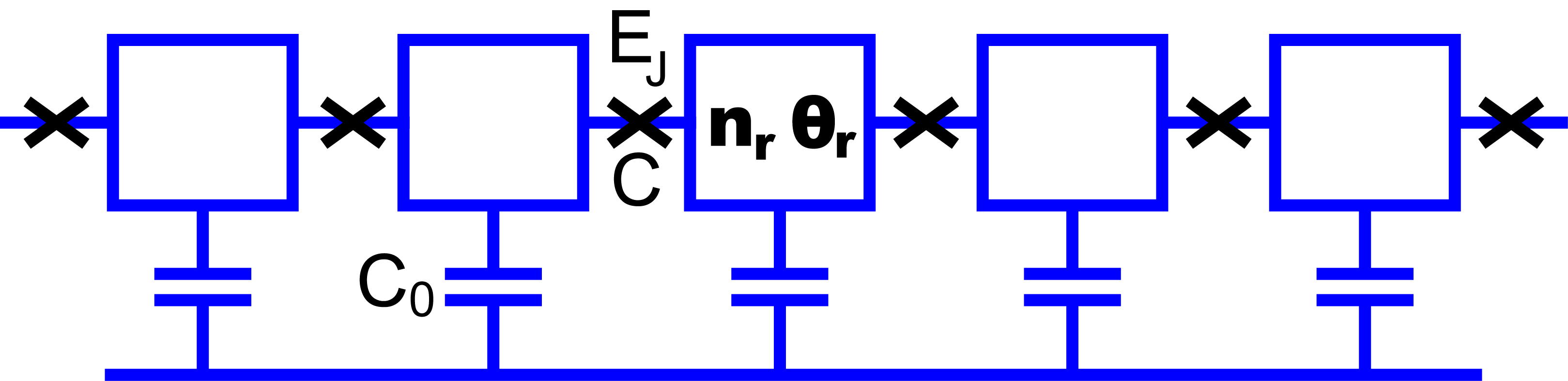
The Josephson junctions with capacitance connect the superconducting grains to each other and each grain has a capacitance to the ground. Typical values are 1fF and aF. The system is governed by the usual Hamiltonian consisting of the Coulomb charging energy (kinetic energy) and the Josephson tunneling (potential energy):
| (1) |
Here are integer-valued island charges (in units of ) and are the corresponding canonically conjugate phases, . The matrix of Coulomb interaction is given by
| (2) |
with being the charging energy and the screening length which determines the spatial extent of the Coulomb interaction. In this paper we consider .
III Tight-binding approach
III.1 Qualitative discussion
In this section we explore the properties of Josephson arrays in the Coulomb blockade regime . We consider the sector of the Hilbert space with exactly one extra Cooper pair in the array. The simplest (and having minimal charging energy) representative of the unit charge sector is the state in which the extra Cooper pair resides on some island with all the other islands being neutral. The charging energy of such a state is given by . This is approximately the energy (rather high!) one has to invest to insert one Cooper pair into the array. Once the Cooper pair has been inserted it is free to move from one site to its neighbor via the hopping provided by the Josephson part of the Hamiltonian. In the limit of vanishingly small only the simplest charge configurations described above are important and we are led to the trivial tight-binding band for an extra Cooper pair in the Josephson chain (cf. [2, 3]).
The peculiarity of the -Josephson chain, first noticed in Refs. [2, 3] and used in Ref. 17, is that the simple picture sketched above is valid only for extremely small . The reason is the presence of a large number of states lying at small energy above the basic states (as opposed to much larger energy which one might expect and which indeed happens in higher dimensions). One particular example is the charge configuration (Cooper pair and a properly oriented dipole nearby) having the energy . Thus, in the parameter range called by the authors of Ref. 17 the small soliton regime, Cooper pair inserted into the chain gets strongly dressed by virtual dipoles and the simplest tight-binding scheme breaks down. Dipole dressing was also mentioned in the context of transport in ion channels [18].
In reference [17] the properties of the small charge solitons were addressed by successive inclusion of the charge configurations (up to states) with larger and larger energies into the tight-binding scheme. A similar scheme was developed for polarons in Ref. 19. In this paper we construct a comprehensive description of the low-lying (with energies much smaller ) states in terms of a particular spin- model. We derive an effective Hamiltonian governing the model dynamics within the low energy subspace. We then develop a tight-binding approach with arbitrary number of the charge states taken into account.
III.2 Structure of the low energy subspace
Let us first define more precisely what we mean under the low lying states in the sector with total charge and construct the complete classification of these states. Let us consider some charge configuration of size . It is clear that the energy of such a configuration will certainly exceed if (from now on we count energies from the energy of a single Cooper pair). Thus for the low-lying configurations and we can expand the charging energy in powers of as
| (3) |
We see that the typical charge configurations have large energy and are not important for the low energy physics. The exceptions are the states nullifying the first term in Eq. (3) and having the energy . Note, that the first term of the expansion (3) can not take negative values. Otherwise there would exist configurations with electrostatic energy smaller than . As long as these charge configurations hybridize effectively with the basic one leading to the formation of the small charge soliton. Thus, the condition
| (4) |
is the mathematical definition of the low energy subspace in the unit charge sector (we call it also the proper space). It can be shown (Appendix A) that the subspace (4) consists of all the configurations with two properties: a) all the islands’ charges equal or ; b) any two charged islands separated by an arbitrary number of neutral islands have opposite charges. For example, the configurations and belong to the low-energy space while the configurations and do not. To describe the proper subspace in a more clear way let us introduce variables defined on the links of the chain (the link is the link connecting islands and )
| (5) |


The connection between variables and charges for two configurations in the low-energy subspace is illustrated in Fig. 2. From the definition of and the properties of the states in the low-energy subspace one immediately concludes that the low-energy configurations are described by for all , i.e., the low-energy subspace is isomorphic to the space of states for a spin- chain with being the z-projections of the spins.
Due to the constraint the variable satisfies the boundary conditions
| (6) |
Thus, extra Cooper pair in the chain is described by a domain wall in the spin language.
III.3 Projecting the Hamiltonian
Having understood the structure of the low-energy space of the model we can project the full Hamiltonian (1) onto the proper subspace. The projection is carried out by noting that Cooper pair tunneling between two neighboring islands corresponds to the spin flip in the link between them. Thus the Josephson part of the Hamiltonian is given by
| (7) |
Rewriting the charging energy in terms of spin variables we arrive at
| (8) |
To determine the spectrum of the single-charge sector of the Hamiltonian (8) we impose the boundary conditions (6) indicating the presence of a domain wall.
The Hamiltonian (8) takes into account the low energy charge configurations of arbitrary width . We understand however that the configurations with are not important at low energies. Thus, we can further reduce the phase space by dropping out all the configurations of the width larger than some . We expect that at the resulting low energy states are independent of and approximate correctly those of Hamiltonian (8).
Any state containing a domain wall of the width less than is completely specified by the position of the first spin up (which we call the coordinate of the charge soliton or domain wall) and the values of the -projections of the next spins . Given the state
| (9) |
one can reconstruct the -projections of all spins in the chain according to
For example, if we choose the states shown on Fig. 2a) and 2b) can be written as
| (15) | |||
| (16) |
In Appendix B we describe how to project the Hamiltonian (8) onto the space of configurations with sizes less or equal than . We also perform a transition from the coordinates to the quasi-momentum . The result reads
| (17) |
where is the operator of the right cyclic shift defined by .
The Hamiltonian (17) constitutes the main result of this section. For it can be shown to produce results equivalent to that of reference [17]. Equation (17) reduces the initial many-body problem to a finite dimensional Hamiltonian, readily accessible to numerics as long as not too large () charge configurations are important. In the next sections we present the results of numerical analysis of the Hamiltonian (17) and compare the results to those of the mean-field approach.
III.4 Results of the tight-binding approach
An example of the band structure obtained within the tight-binding approach is shown in Fig. 3. In Fig. 4 the two lowest bands are shown.


We observe that the lowest band is parabolic for small momenta and flattens in the outer part of the Brillouin zone. This phenomenon was already observed in Ref. 17. To further emphasize the dispersion relation of the lowest band in Fig. 5 we show the group velocity of the soliton (dressed Cooper pair) as compared to the one of an undressed Cooper pair. We find that the flattening of the dispersion relation in the outer region of the Brillouin zone leads to zero group velocity.

In this paper we concentrate mostly on the investigation of the effective mass of the charge carriers. In the tight-binding approach we define , where is the dispersion of the lowest band (ground state). In what follows we will compare this mass with the results of the mean-field theory.
III.4.1 Persistent current
As a first obvious application of our results consider a ring-shaped array of junctions with exactly one extra Cooper pair in it. If an external magnetic flux is applied a persistent current will emerge. The periodic boundary condition for the Bloch wave with wave vector reads
| (18) |
Thus, as the external flux varies between and , the relevant wave vector varies between and . For large enough the interval is safely within the domain of parabolic dispersion relation. Thus we use the effective mass approximation and obtain for the persistent current in the interval
| (19) |
where is the effective mass of the charge carrier (in the tight-binding approach we obtained ). Thus, the amplitude of the persistent current oscillations is given by
| (20) |
With no polaronic effects taken into account, i.e., for a bare Cooper pair we would have and . Thus we obtain
| (21) |
where is the critical current of a single Josephson junction. We observe that the effective mass reduction via the polaronic effects enhances the persistent current.
IV Mean-Field Theory
IV.1 Description in terms of continuous polarization charges
An alternative description of the charge propagation in the array is given in terms of the continuous polarization charges, e.g., the screening charges on the gate capacitances (see Fig. 6). For the system described in the previous section the continuous polarization charges are enslaved to the discrete charges . That is, once a tunneling process occurs and the distribution changes, the polarization charges adjust immediately to the new situation. To allow formally independent dynamics of polarization charges we introduce infinitesimal inductances as shown in Fig. (6).

This leads to two independent degrees of freedom per cell of the array. One quantized charge degree of freedom is the number of Cooper pairs that have tunneled through junction number . Its conjugate phase is given by and the commutation relations read . The second continuous charge degree of freedom is equal to the polarization charge that has arrived at the junction number or, alternatively, the integral of the displacement current flowing into junction . The conjugate variable is the magnetic flux on inductance in cell number . The commutation relation reads . We obtain the following Hamiltonian of the array
| (22) | |||||
IV.2 Mean-field approximation
The mean-field description is based on the Heisenberg equations of motion for the polarization charge following from (22):
| (23) |
We average Eq. (23) over the state of the system and obtain
| (24) |
where is the expectation value of the voltage drop across junction number . In the mean-field approximation we calculate by replacing the operators by their average values in the Hamiltonian (22). Thus the problem factorizes to many single-junction ones. Each junction is governed by the Hamiltonian
| (25) |
where we have dropped the index . The gate charge is a given function of time (to be replaced in each junction by ). For the expectation value of the voltage we then obtain . The problem is now to find the quantum state of the junction in which the average should be evaluated. We do so assuming that is a slow function of time. This assumption should be checked for self-consistency later.
The Hamiltonian (25) possesses the (adiabatic) spectrum with discrete eigenvectors obeying and eigenvalues , cf. Fig. 7. The general wave function is a superposition .

Our aim is to determine for a given function . We restrict ourselves to the adiabatic case, i.e., we keep only terms of order . After a calculation presented in Appendix C we arrive at
| (26) |
Here we defined the Bloch inductance first introduced by Zorin [15]:
| (27) |
(In Ref. 15 only the first excited state () in (27) was taken into account and the contribution in (26) was omitted.) For the Bloch inductance is sharply peaked around (see Fig. 8). In the opposite case, , the Bloch inductance is nearly constant, .

Combining Eq. (26) and the self-consistency equation (24) we obtain
| (28) |
where we substituted for clarity. We observe that the kinetic inductance is superseded by the Bloch inductance at least around and we can safely assume . Yet, in the regime , when is exponentially small in the regions and , a finite geometric or kinetic inductance could be important. In the continuum limit, i.e., after the substitution , equation (28) reads
| (29) |
We now make the very important observation that (29) is the equation of motion for the following Lagrangian density
| (30) |
In the limit , when and we obtain the usual sine-Gordon equation. On the other hand, in the limit equation (29) differs in several aspects from the sine-Gordon equation: i) The first two terms of (29) describe a wave guide with a -dependent “light velocity” . With the Bloch inductance having a peak value at we obtain the minimal light velocity . ii) The ground state energy is still a periodic function of but it is no longer proportional to . iii) Since depends strongly on , the third term of (29) is very important.
IV.3 Solitonic solutions
We are now searching for a solitary wave traveling with velocity by plugging the ansatz into Eq. (29). This gives the following differential equation
| (31) |
Integrating we obtain
| (32) |
Here, is an integration constant and stands for the soliton / antisoliton solution. We impose the boundary conditions and to describe the propagation of a single Cooper pair in the array. This also fixes the integration constant, . The solitonic solutions only exist for .
IV.4 Lorentz contraction
In the limit , Eq. (29) reduces to the sine-Gordon equation and is Lorentz invariant. Thus solitons undergo the usual Lorentz contraction. In the other limit, , Eq. (29) is not Lorentz invariant. The Lorentz contraction of the soliton takes a very peculiar shape. Consider a soliton moving with velocity approaching (we postpone for a moment a discussion on whether this is consistent with adiabaticity). For the center of the soliton, where , the relativistic regime is reached and it is Lorentz contracted (see Fig. 9). In contrast, the soliton’s tales, where or are unaffected by Lorentz contraction.

IV.5 Rest energy and dynamical mass of the soliton
Using the Lagrangian density (30) we find the energy of a soliton
| (33) |
For small velocities we expand and obtain . The rest energy of the soliton is given by
| (34) |
For the kinetic mass we obtain
| (35) |
In the limit , when , we obtain as expected the relativistic relation (in this limit the light velocity is -independent, ).
In the opposite charging limit, , no such relativistic relation exists. A simple estimate then gives
| (36) |
consistent with the result of Sec. III.1.
In the limit the Bloch inductance is sharply peaked around and the integral of Eq. (35) is dominated by a small vicinity of this point. Here a two-state approximation is valid which gives with . As is sharply peaked around , we can replace in (35) by its value at , , leading to
| (37) |
where is the ”naive” tight-binding mass of a single Cooper pair. The polaronic reduction of the mass is evident from (37) in the regime .
IV.6 Comparison with the tight-binding results
In Fig. 10 the mass obtained in the mean-field approach is compared with the mass from the tight-binding calculation.

We observe a good correspondence for . This is the main result of this paper. The mass scales approximately as . As the convergence of the tight-binding approach gets worse with raising ratio we also show the uncertainty of the result by giving the upper boundary for (upper dashed curve in Fig. 10).
IV.7 Adiabaticity condition and the validity of the mean field theory
The analysis above rests on two assumptions: a) the dynamics of is slow and allows us to neglect the Landau-Zener tunneling in the derivation of Eq. (26); b) the field can be regarded as classical.
Since in terms of the solitons are large objects (with the size of the order of ) one can expect the second assumption to hold in a wide parameter range. In particular, at we can estimate the “effective Planck constant” [20] for the Lagrangian (30) as
| (38) |
While at small enough strong suppression of the nonlinear Bloch inductance for may become important, we expect this effect to be of minor significance in the intermidiate range of .
The situation with the assumption a) is much more tricky. First of all, the adiabaticity imposes an upper boundary for the velocity of solitons to be considered. In the limit the probability of a Landau-Zener transition into the first excited level is given by
| (39) |
where , is the difference of the charging energies of the two charge states involved in the process. Thus, and . If we demand , the corresponding limitation on the soliton’s velocity reads
| (40) |
We see that for , the maximal velocity for which adiabaticity still holds goes to zero.
It is obvious that even for a static soliton the adiabaticity condition can be broken by fluctuations around the saddle point. Thus, the precise determination of the applicability region for the adiabatic approximation requires understanding of the characteristic time scale for the two-point correlation function of with the account of the nonlinear Bloch inductance. However, the good agreement between the mean-field theory and the tight-binding approach found in the calculation of the soliton mass for intermediate allows us to expect that adiabaticity indeed holds in this parameter range for small soliton velocities.
V Conclusions
In this paper we studied the dynamical properties of the charge carriers (charge solitons) in infinite one-dimensional Josephson arrays without disorder. We applied two complementary techniques and arrived at our main result: in the parameter regime the polaronic effects strongly reduce the effective mass of the charge solitons which scales approximately as .
VI Acknowledgements
We thank M. Berry, A. Ustinov, H. Rotzinger, R. Schäfer for numerous fruitful discussions. IP acknowledges support from the German-Israeli Foundation (GIF). SR acknowledges support from the Deutsche Forschungsgmeinschaft (DFG) under Grant No. RA 1949/1-1.
Appendix A Low lying excitations and the spin formulation
The aim of the present Appendix is to find an explicit description of the low energy charge configurations satisfying the constraint
| (41) |
Let us consider one such configuration. We try to add a dipole at islands and to this configuration, i.e. we construct a new configuration given by
| (42) |
For the new configuration to belong to the low lying sector we need the following condition to hold:
| (43) |
We can rewrite this condition as
| (44) |
In terms of the spin variable introduced in Sec. III.2, Eq. (44) is equivalent to the condition
| (45) |
After the creation of an additional dipole (i.e. the Cooper pair tunneling from island to island ) the new state is described by
| (46) |
We thus conclude that the Cooper pair tunneling from island to island is allowed (i.e. drives the system into another state within the low energy subspace) if . Such a tunneling corresponds to the spin flip at the link connecting the island and . It is easy to check that the inverse process (tunneling from to ) is allowed only when and also leads to the flip of . Taking into account that a single Cooper pair at island is described in terms of by a domain wall
| (47) |
we conclude that the low energy configurations are those with for all Translated into the charge language this condition gives the conditions mentioned in the main text (Sec. III.2).
Appendix B Projecting the Hamiltonian
We consider the action of the Josephson term in the Hamiltonian (8) on the state (9). Obviously, we can drop all the terms with or from the sum over since acting on the state (9) they inevitably create the configuration of the width greater than . The terms with do not change the position of the first spin up in the chain and, thus, the coordinate of the soliton . Thus, their action is described by
| (48) |
We consider now the action of . It is convenient to introduce the operator of the right cyclic shift acting on the states according to
| (49) |
Assume that in the state exactly first spins are down () (we require now ; the case of spins down will be considered separately). The direction of other spins is arbitrary. In this case the action of on our state is given by
On the other hand, if in the given state exactly first spins are , then
| (51) |
Thus we conclude that for any state (except the state with all spins down)
Finally, taking into account that
| (53) |
we find for the projection of onto the space spaned by the configurations of the width less or equal than
| (54) |
The last part of the Josephson Hamiltonian
| (55) |
after the projection onto the subspace of interest, produces an expression conjugate to (54). Thus, summing up all the contributions we find the projected Josephson Hamiltonian
| (56) |
Going to the momentum domain with respect to the cyclic coordinate and performing some simplifications based on the elementary properties of and , we finally arrive at Eq. (17).
Appendix C Adiabatic calculation
The most direct way is to apply the time-dependent perturbation theory. We will instead use a technique proposed by Berry [21] where we apply several unitary transformations, so that the eigenstates of the transformed Hamiltonians approach asymptotically the actual evolving state.
We consider the adiabatic case and the terms of orders higher than are omitted. The general transformation reads
| (57) |
with being the time-dependent unitary operator that diagonalizes at each time . We can write
| (58) |
where are the eigenvectors satisfying
| (59) |
and time-independent vectors can be chosen arbitrarily, e.g., . We now perform the first step of this process explicitly. As Hamiltonian we take (25) with . From (58) we find
| (60) |
Applying (57) gives the transformed Hamiltonian
| (61) |
We find by applying the usual time-independent perturbation theory with the perturbation being the second term on the RHS of (61). This gives the new transformation matrix because , which can be used for a second transformation to obtain with eigenvectors . After calculating we can go back to the desired basis via
| (62) |
Putting everything together gives
| (63) |
with and .
We are now able to calculate the voltage with , where we set in (63) as we consider our system being initially in the ground state. We use and and arrive
at Eqs. (26,27).
References
- [1] R. M. Bradley and S. Doniach, Phys. Rev. B 30, 1138 (1984).
- [2] A. A. Odintsov, JETP Lett. 60, 738 (1994).
- [3] A. A. Odintsov, Phys. Rev. B 54, 1228 (1996).
- [4] D. B. Haviland and P. Delsing, Phys. Rev. B 54, R6857 (1996).
- [5] Z. Hermon, E. Ben-Jacob, and G. Schön, Phys. Rev. B 54, 1234 (1996).
- [6] L. I. Glazman and A. I. Larkin, Phys. Rev. Lett. 79, 3736 (1997).
- [7] D. B. Haviland, K. Andersson, and P. Ågren, J. of Low Temp. Phys. 118, 733 (2000).
- [8] P. Ågren, K. Andersson, and D. B. Haviland, J. of Low Temp. Phys. 124, 291 (2001).
- [9] V. Gurarie and A. Tsvelik, J. of Low Temp. Phys. 135, 245 (2004).
- [10] K. B. Efetov, Sov. Phys. JETP 51, 1015 (1980).
- [11] J. E. Mooij, B. J. van Wees, L. J. Geerligs, M. Peters, R. Fazio, and G. Schön, Phys. Rev. Lett. 65, 645 (1990).
- [12] M. P. A. Fisher, Phys. Rev. Lett. 65, 923 (1990).
- [13] R. Fazio and G. Schön, Phys. Rev. B 43, 5307 (1991).
- [14] R. Fazio and H. van der Zant, Phys. Rep. 355, 235 (2001).
- [15] A. B. Zorin, Phys. Rev. Lett. 96, 167001 (2006).
- [16] C. Hutter, A. Shnirman, Y. Makhlin, and G. Schön, Europhys. Lett. 74, 1088 (2006).
- [17] S. Rachel and A. Shnirman, Phys. Rev. B 80, 180508 (2009).
- [18] J. Zhang, A. Kamenev, and B. I. Shklovskii, Phys. Rev. Lett. 95, 148101 (2005).
- [19] J. Bonča, S. A. Trugman, and I. Batisti, Phys. Rev. B 60, 1633 (1999).
- [20] S. Coleman, Phys. Rev. D 11, 2088 (1975).
- [21] M. V. Berry, Proc. R. Soc. Lond. A 414, 31 (1987).