.
Superconductivity in the two-dimensional Hubbard model based on the exact pair potential
Abstract
We analyze solutions to a superconducting gap equation based on the two-dimensional Hubbard model with nearest and next-to-nearest neighbor hopping. The Cooper pair potential can be calculated exactly and expressed in terms of standard elliptic functions. The Fermi surfaces at finite temperature and chemical potential are also calculated based on the exact two-body S-matrix of the Hubbard model using the formalism we recently developed[7], which allows variation of hole doping. The resulting solutions to the gap equation are strongly anisotropic, namely largest in the anti-nodal direction, and zero in the nodal directions of the Brillouin zone, but not precisely d-wave. For and , appropriate to BSCO, and a physically natural choice for the cut-off, our self-contained analytic calculations yield and maximum at optimal hole doping . For phenomenological fits to the Fermi surfaces for cuprates, we obtain the comparable value at optimal doping, both in good agreement with experiments. The superconducting gap is non-zero for all hole-doping and increases all the way down to zero doping, suggesting that it evolves smoothly into the pseudogap.
I Introduction
The microscopic physics underlying high superconductivity in the cuprates is believed to be purely electronic in origin, and strongly correlated electron models such as the two-dimensional Hubbard model have been proposed to describe it[1]. A partial list of more recent articles addressing the existence of superconductivity in the Hubbard model is [2, 3, 4], and references therein. The Hubbard model simply describes electrons hopping on a square lattice subject to strong, local, coulombic repulsion. Since it is known that the condensed charge carriers have charge , and thus some kind of Cooper pairing is involved, a central question has become “What provides the glue that pairs the electrons?”. This is especially puzzling since the underlying bare interactions are repulsive. The situation is completely different in the Bardeen-Cooper-Schrieffer (BCS) theory of ordinary superconductors, where the attractive glue is provided by the interaction of the electrons with the lattice phonons[5].
Since the Mott-insulating anti-ferromagnetic phase at half-filling is well understood, a large portion of the theoretical literature starts here and attempts to understand how doping “melts” the anti-ferromagnetic order, and how the resulting state can become superconducting. This has proven to be quite challenging, perhaps in part due to the fact that anti-ferromagnetic order is spatial, whereas superconducting order is in momentum space. Consequently this has led to many interesting and in cases exotic ideas, however the central question, “What is the glue?”, and how it arises from strongly coupled physics, remains unclear. (For a review and other refereces, see [6].) This suggests that it may be more fruitful to begin on the overdoped side, far away from any competing anti-ferromagnetic order, in order to understand the attractive mechanism in a pure form. Here the density is perhaps low enough that one can treat the model as a gas, with superconductivity arising as a condensation of Cooper pairs as in the BCS theory, and we will adopt this point of view in the present work. The observation made in [7] now comes to bear on the problem: multi-loop quantum corrections to the scattering of Cooper pairs can actually lead to effectively attractive interactions, even though the bare model was defined with repulsive interactions. In the work [7], the focus was on the thermodynamics at finite temperature and chemical potential, and evidence was presented for instabilities toward the formation of new phases as the temperature was lowered. However our purely thermodynamic formalism was unable to probe the nature of the ground states of these potentially new phases. The present work attempts to complete the picture. Namely, we explore how the attractive interactions described in [7] can lead to superconductivity, and what its basic properties are.
Our starting point will be the BCS theory, but specialized to the Hubbard model. The original Cooper argument[8] is quite robust, and shows that any attractive interactions near the Fermi surface lead to a pairing instability. We thus assume that the BCS construction of the ground state goes through, leading to the well-known gap equation[5]:
| (1) |
Here, is the energy gap, is the energy of excitations above the ground state, and is the temperature. We will later make some favorable checks on the approximations that lead to the above equation. In the above gap equation, represents the residual interaction of Cooper pairs, and we will refer to it as the (Cooper) pair potential. The main new input is that we compute from the Hubbard model, including quantum corrections, and show that it has attractive regions in the Brillouin zone. The other ingredient is , which represents normal state quasi-particle energies near the Fermi surface, where at the Fermi surface. This can be identified with the “pseudo-energy” in the thermodynamic approach described in [7]. These two ingredients lead to a self-contained analysis of the solutions of the above gap equation based entirely on analytic calculations carried out in the Hubbard model.
An outline of the sequel, along with a summary of our results, goes as follows. In the next section we describe our conventions for the Hubbard model, with hopping strengths and the repulsive coupling , all with units of energy. The pair potential is calculated in section III by summing multi-loop Feynman diagrams; the final result is expressed in terms of elliptic functions. It is demonstrated that, rather surprisingly, when is large enough, there opens up a region of attractive interactions, i.e. negative , near the half-filled Fermi surface. In section IV, the method developed in [9, 7] for the thermodynamics is reviewed, and Fermi surfaces are calculated as a function of doping for and , appropriate to the cuprate BSCO. The results in these sections III, IV constitute the main inputs for the study of the solutions of the gap equation, which is carried out in section V. The values we compute for the gap and are in reasonably good agreement with experiments. The gap is anisotropic, in that it vanishes in the nodal directions and is largest in the anti-nodal, however it is not precisely of d-wave form. Our solutions to the gap equation persist to arbitrarily low doping, and we propose that they evolve into the so-called pseudogap, in accordance with recent experiments. In section VI, we repeat the analysis of the gap equation using a phenomenological fit to the Fermi surfaces.
II The Hubbard model gas
The Hubbard model describes fermionic particles with spin, hopping between the sites of a square lattice, subject to strong local coulombic repulsion. The lattice hamiltonian is
| (2) |
where are sites of the lattice, denotes nearest neighbors, are densities, and satisfy canonical anti-commutation relations. We have also included a next to nearest neighbor hopping term , since it is not difficult to incorporate into the formalism, and it is known to be non-zero for high materials.
The free part of the hamiltonian, i.e. the hopping term, is easily diagonalized:
| (3) |
with the free 1-particle energy
| (4) |
where taken to be positive. In the sequel it is implicit that is restricted to the first Brillouin zone, , where is the lattice spacing.
Since the quartic interaction is local, we introduce the two continuum fields and the action
| (5) |
where is the hamiltonian density. The field has the following expansion characteristic of a non-relativistic theory since it only involves annihilation operators,
| (6) |
and satisfies at equal times . Since we have represented sums over lattice sites as , where is the lattice spacing, . The interaction part of the hamiltonian is approximated as a continuum integral with density
| (7) |
where . Formally, the free part of the hamiltonian density is , where is the differential operator , and is thus non-local. However this non-locality does not obstruct the solution of the model since the free term can be diagonalized exactly. The model can now be treated as a quantum fermionic gas, where the only effect of the lattice is in the free particle energies .
The field has dimensions of inverse length, and the coupling units of . In the sequel we will scale out the dependence on and the lattice spacing , and physical quantities will then depend on the dimensionless coupling
| (8) |
Positive corresponds to repulsive interactions. Henceforth, all energy scales, in particular, the single particle energies , the gap , temperature, and chemical potential, will be implicitly in units of .
For both cuprates LSCO and BSCO, , , and approximately equals and respectively. Therefore, for most of the detailed analysis below, we set and appropriate to BSCO.
III The Cooper pair potential .
The kernel in the gap equation (1) represents the residual interaction of Cooper pairs of momenta and . It is related to the following matrix element of the interaction hamiltonian:
| (9) |
To lowest order, is momentum independent: .
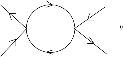
In quantum field theory, the above matrix element of operators, in this case , is generally referred to as a form-factor. Since there is no integration over time, this form-factor does not conserve energy, i.e. there is no overall -function equating to . The form-factor can be calculated using Feynman diagrams as follows. More generally consider the form-factor . Represent the interaction vertex with two incoming arrows for the annihilation operator fields and two outgoing arrows for the creation fields . Furthermore, let such a vertex with a “node” represent the operator . Then is given by the sum over diagrams shown in Figure 1, where represents energy-momentum.

Momentum is conserved at each vertex, however energy is not conserved at the vertex with a node. There is actually no fermionic minus sign associated with each loop since the arrows do not form a closed loop. Diagrams with a closed loop, such as in Figure 2, are zero because the integration over energy inside the loop has poles in the integrand that are either both in the upper or lower half-plane, so that the contour can be closed at infinity without picking up residues. In other words, there is no “crossing-symmetry” as in relativistic theories. (For the contrary, see the non-zero loop integral below.) This fact, which is unique to non-relativistic theories, allows us to calculate the kernel exactly. At order , specializing to Cooper pairs and , the diagram in Figure 1 factorizes and contributes
| (10) |
where is a 1-loop integral
| (11) |
where and are the total incoming energy and momentum, i.e. and . As usual, is infinitestimally small and positive. The extra is due to the over-counting by allowing each loop to be or . Finally, summing over gives
| (12) |
It is important to note that the above is exact and has a smooth limit, i.e. it allows an expansion in the inverse coupling , so is in a sense non-perturbative. One may be concerned that we formally summed a geometric series that potentially does not converge. In answer to this, there are certainly regions where is small enough that the series converges. Also, this summation is known to give the correct, exact, S-matrix for non-relativisitic quantum gases, and this S-matrix has all of the right properties in the strongly coupled unitary limit[10], namely, it gives the correct diverging scattering length at the renormalization group fixed point, and the bound state. The only difference here is that the the kinetic energy is replaced with for the Hubbard model, which does not affect these arguments.
The -integral can be performed by deforming the contour to infinity, giving . Note is imaginary as , thus in the formula (12), is really the imaginary part of as such that is real. Then, integral over can be performed analytically[7]:
| (13) |
with , where is the complete elliptic integral of the first kind. Note that the momentum dependence of the kernel only enters through the variables , i.e. .
Non-zero solutions to the gap equation possibly signifying superconductivity can only arise if the effective interactions are attractive, i.e. if the kernel is negative. For small and positive, the effective coupling remains repulsive. However, as pointed out in [7], for large enough, can become negative in certain regions of the Brillouin zone. Since we are interested in a small band of energies near the Fermi surface, with is a suitable probe of these attractive regions. In Figure 3 we plot this for and at fixed . One sees that for the smaller , is everywhere positive, however for larger it flips sign. As explained in more detail in [7], this feature is reminiscent of what occurs near the fixed point of quantum gases in the unitary limit, where for the same analytic reasons, the effective interactions can be either attractive or repulsive depending on which side of the fixed point of the BEC/BCS crossover[10]. Using the formula (13), one can show that there is a region of negative for . This minimal value of depends on and this dependence was studied in [7] based on the formula (13). Around , the attractive region is a narrow band[7]. It will also be instructive to view a contour plot of in the first Brillouin zone, see Figure 4.


The main effect of a non-zero is the following. For large enough, becomes negative for . Thus when is negative and large, attractive interactions exist deeper inside the half-filled Fermi surface. If superconductivity indeed arises from these attractive interactions, then a non-zero can play a significant role, otherwise the attractive interactions only exist too close to the vicinity of the half-filled Fermi surface where it has to compete with the known Mott-insulator phase. There is actually some evidence that superconductivity does not exist for [11].
IV The Fermi surfaces as a function of doping
We will utilize the approach to the thermodynamics of particles developed in [9, 7], which is based on a self-consistent re-summation of the exact 2-body scattering. The occupation numbers are parameterized by two pseudo-energies , which satisfy 2 coupled integral equations with a kernel related to the scattering of spin up with spin down. For equal chemical potentials, due to the SU(2) symmetry, , and both occupation numbers are given by
| (14) |
where satisfies the single integral equation:
| (15) |
The kernel is related to the logarithm of the 2-body S-matrix, and is built from the same ingredients as the kernel in the gap equation, since it also involves a sum of Feynman diagrams of the kind shown in Figure 1. It is somewhat more complicated than the pair potential since the total incoming momentum is not zero. Namely, consider the same loop integral as in the previous section but with :
| (16) |
where and are defined to be real. Then the kernel takes the following form
| (17) |
where the renormalized coupling is . (We are not displaying the momentum dependence; it is implicit that .) The renormalized coupling is related to the gap equation kernel of the last section as follows: . The quantity represents the phase space available for 2-body scattering. The argument of the is the exact 2-body S-matrix.
We define the hole doping as the number of holes per plaquette, which is related to the density as follows:
| (18) |
where is the lattice spacing.
The integral equation (15) was solved numerically using an iterative procedure, as explained in [7]. The solution for the pseudo-energy yields the relation between the chemical potential and the hole doping . For a given , of course depends on temperature, but only weakly[7]. For the subsequent analysis we determine at the low reference temperature . The result is shown in Figure 5.

As described in [7], for low enough , there are regions of where there are no solutions to the integral equation at low enough . Regions of the non-existence of solutions are very similar to that shown in Figure 8 in[7], For hole dopings , there are no solutions for temperatures in the range . (This is why we chose the reference temperature to be above these potential transition temperatures.) It was suggested in [7] that the non-existence of solutions could represent an instability toward the formation of a new phase, however the nature of these new phases cannot be determined based on what we have done so far; one needs a complementary bottom up approach that is based on the zero temperature ground state. This is the subject of the next section. As we will see, the critical temperatures inferred from this thermodynamic analysis are consistent with the critical tempertures computed from the gap equation in the next section.
The Fermi surfaces are the contours that are solutions to , where depends on hole doping as in Figure 5. The pseudo-energy thus represents the quasi-particle dispersion relation in the normal state. These Fermi surfaces are shown in Figure 6 for . These calculated Fermi surfaces are in reasonably good agreement with experiments. Comparison with Figure 10, which is based on a phenomenological fit to the data, suggests that one needs to include additional hopping terms in the bare hamiltonian, such as next-to-next neighbor. We will refer to wave-vectors that point to (and rotations thereof) as being in the nodal direction, whereas those pointing to as in the anti-nodal direction.
In the same Figure 6 we also display the region of attractive interactions based on the Cooper pair potential calculated in the last section. Before even solving the gap equation, one can make some predictions concerning the existence of superconductivity based on the attractive region of . Namely, for high enough hole doping, about , there is no attractive region near the Fermi surface, and thus no superconductivity. It is also clear from Figure 6 that the regions of the Fermi surface in the anti-nodal direction are the most important since this is the direction with the greatest overlap with the attractive region. As we will show in the next section, this feature is primarily responsible for the anisotropy of the gap , and explains why the gap is zero in the nodal direction, at least for moderately high doping .

V Solutions to the gap equation
The gap is defined and measured for along the Fermi surface. However near half-filling, there is no from the origin that intersects the Fermi surface in the anti-nodal direction; see Figure 6. Consequently, polar plots of for originating from the center of the Brillouin zone, and covering all of it, are potentially misleading, since is not well-defined in the anti-nodal directions. In fact, this also implies that cannot be strictly d-wave as defined from the origin, for example, it cannot be of the simple form , where is measured from the origin. Thus, in the first quadrant of the Brillouin zone, it is more convenient to work with the vector originating from the node , i.e. , where .
In the integral gap equation (1), one must integrate over a narrow band around the Fermi surface . Let be the angle of relative to the horizontal line through the node: . If the integration is over a narrow band of width around the Fermi surface, then the gap equation takes the following form in the first quadrant:
| (19) |
where , and is the length of along the Fermi surface. Here is the negative (attractive) part of since only when is negative are there solutions; the repulsive parts of are already incorporated in determining the Fermi surfaces. The doping dependence of the above equation is implicit in .
It remains to determine the cut-off . There is some arbitariness in the choice of , and this is the weakest aspect of our calculation since certainly depends on it, just as depends on the Debye frequency in ordinary superconductors. It could be viewed as a free parameter that needs to be fit to the data. Or, one could carry out a sophisticated renormalization group analysis requiring to be independent of , but this is at the expense of introducing an arbitrary scale that has to be fit to experiments. Instead, we found the following choice to be physically meaningful and well-motivated. As in the BCS theory, should be related to the properties of the potential itself, namely the region in which it is attractive relative to the Fermi surface11 1 In the BCS theory, the cut-off is the Debye frequency , and is a measure of the width of the attractive region.. Define such that is attractive for in the nodal direction. For , . We then take as a measure of the distance of the Fermi surface to the edge of the region of attractive interactions in the nodal direction: . From the Figure 6, one sees that is quite small, so that our choice does correspond to a narrow band. For the Fermi surfaces computed in the last section, for doping and this value will be used in the subsequent analysis.
The function in the gap equation represents the quasi-particle dispersion relation of the normal state, and is zero along the Fermi surface. We wish to carry out a self-contained calculation, thus we equate with the pseudo-energy of the last section. On the other hand, one can infer from experiments, and we will repeat the analysis with such a in the next section.
A measure of the validity of the BCS approximation is the combination of the effective coupling and the phase space integration in the gap equation, i.e. the parameter . From Figure 3, , and also . This gives , which appears to be sufficiently small for the BCS approximation to be valid.
We solved the gap equation numerically by discretizing the integrals and solving the resulting set of coupled non-linear equations with Mathematica. In Figure 7 we plot the zero temperature gap as a function of the Fermi surface angle for 3 different hole dopings. One sees that is highly anisotropic in the Brillouin zone: it is largest in the anti-nodal directions, and zero in the nodal direction for high enough doping. At low doping, the anisotropy is less pronounced. This property can be traced to the detailed shape of the Fermi surface in comparison to the region of attractive interactions displayed in Figure 6. More specifically, for high enough doping, the Fermi surface does not intersect the region of negative in the nodal direction, however it always does in the anti-nodal direction. This effect is even more pronounced for the experimentally determined Fermi surfaces, as will be described in the next section.
Our solutions to the gap equation are not exactly d-wave, more specifically, are not proportional to , which is approximately , for the Fermi surface approximated as a circle of radius . Experimental data indicates a gap closer to the d-wave form, however some data does show a tendency for it to flatten out in the nodal direction, as in our solutions. However the precise shape of the gap as a function of will change if the cut-off is made to depend on , instead of a simple constant as we have done here. Some features in Figure 7 are reflected in the data[14], in particular, the central region around where the gap is smallest widens with increasing doping. We also wish to point out that our Figure 6 is suggestive of an observation made in [14]: the Bogoliubov quasiparticle interference, indicative of the existence of Cooper pairs, disappears along the diagonal line connecting the two anti-nodes and . (See Figure 3 in [14].) Interestingly, this diagonal line is very close to the contour that separates attractive from repulsive regions of the pair potential, however we are unable to make a direct connection at present. These observations are more pronounced in Figures 11 and 10.

The gap in the anti-nodal direction is plotted as a function of temperature for in Figure 8. Where it goes to zero defines , in this case . Our results for the zero temperature gap in the anti-nodal direction and for various doping are summarized in the table below. Figure 9 plots both the zero temperature gap and as a function of doping. Moving down from the overdoped side, the maximum occurs first at , in good agreement with experiments. For , one obtains and at , compared with the experimental values and for BSCO.


As explained in the last section, there is a succinct reason for why there is no superconductivity at high enough doping, roughly , since beyond this, no part of the Fermi surface overlaps with . See Figure 6. A slightly lower value of is more typical in experiments. However there is no mechanism in the gap equation to turn off the gap at low enough doping, and it continues to increase all the way down to zero doping. Superconductivity would turn off if were smaller, namely around , since in this case the region of attractive interactions is a narrow band, and at low enough doping the Fermi surface does not overlap with it[7]. However if eq. (8) is accurate, is roughly twice as large, so this does not account for the disappearance of superconductivity at low doping. Although this may appear problematic when one compares with the usual phase diagram of the cuprates, there is growing experimental evidence that this is actually the correct behavior[14, 15]. Namely, it has recently been found that the d-wave superconductivity gap evolves smoothly into a d-wave pseudogap whose magnitude continues to increase to arbitrarily low doping, where superconductivity is not present. In other words, the so-called pseudo-gap energy scale may be the continuation of the superconducting gap, had there been no other other mechanisms to destroy it. As stated explicitly in [15], these results are inconsistent with 2-gap scenarios. One check of this is that if one identifies with , then for at doping , again in reasonable agreement with experiments. This suggests that on the underdoped side, superconductivity is perhaps destroyed by competition with other orders, presumably anti-ferromagnetic, bringing to zero, even though the gap is still physically present. It could also be destroyed by phase decoherence, as suggested in[16, 17]. These effects are of course not implemented in our gap equation, and it is beyond the scope of this paper to address this, for example by comparing the free energies for the competing orders or to study to phase fluctuations.
VI Solutions to the gap equation for phenomenologically determined Fermi surfaces
In this section we repeat the analysis of solutions of the gap equation with the normal state quasi-particle dispersion relation determined from experimental data, but with the same pair potential computed in section III. There is extensive data on the Fermi surfaces for the compound . A tight-binding fit to the data was performed in [12] based on the data in [Ding]. The result is that the Fermi surfaces are the contours for the following function:
| (20) | |||||
We have rescaled the result for in [12] so that . The parameter serves as a renormalized chemical potential. For hole dopings , , respectively.
Let us assume that the underlying Hubbard hamiltonian has the same , i.e. , and still only has nearest and next-nearest neighbor hopping parameters and , where from eq. (20) one reads off . The other terms in eq. (20) should be viewed as generated by the interactions, for example by equations such as in section IV for the pseudo-energy . In Figure 10 we display the resulting Fermi surfaces against the region of attractive interactions as computed in section III, but with . In comparison with Figure 6, one sees that the effect that leads to the anisotropy of the gap is more pronounced: the Fermi surfaces are pulled away from the attractive region in the nodal direction in a stronger manner, which implies that the gap will continue to be zero in the nodal direction for lower values of in comparison to the last section.

In Figure 11 we plot the solution to the gap equation for . The same cut-off as in the last section was used. For the reasons stated above, the gap is zero for a wider region centered at . Plots of the gap as a function of temperature are very similar to those of the last section, and lead to a slightly lower , i.e. at optimal doping .

VII Conclusions
The central proposal of this work is that quantum loop corrections to the Cooper pair potential, as computed here in the two-dimensional Hubbard model, could be responsible for the effectively attractive interactions near the Fermi surface that lead to the phenomenon of high superconductivity. The validity of this idea is easily explored, since the pair potential can be calculated exactly, and the results favor our proposal. We showed that the resulting analysis of the solutions to the superconducting gap equation leads to definite predictions for the anisotropy of the gap, its magnitude, and , all in reasonably good agreement with experiments. We explained in a clear manner why superconductivity disappears at high enough doping; in our calculation .
We found that the non-zero solutions to the gap equation continue undiminished on the underdoped side, all the way down to zero doping, and this appears to be consistent with recent experimental results[14, 15], with the interpretation that the d-wave superconductivity gap evolves smoothly to the d-wave pseudogap. If the attractive interactions considered in this paper are indeed responsible for superconductivity, then this feature suggests two items on the more speculative side:
On the underdoped side, superconductivity is perhaps destroyed by competition with the anti-ferromagnetic phase which is known to exist at very low doping. Here one must bear in mind that we kept only the attractive part of the pair potential for the superconducting gap equation, but inside the Fermi surface the interactions are still largely repulsive. Another possibility is that it is destroyed by phase decoherence of the gap[16, 17].
The pseudo-gap energy scale may thus represent the hypothetical continuation of the superconducting gap had it not been destroyed by the mechanisms suggested above. If one identifies with , then for at zero doping, again in reasonable agreement with experiments.
If these ideas are correct, then the emphasis should shift from trying to understand “doping the Mott insulator” to its opposite, that is to say, understanding how populating the superconducting state can destroy it due to the competing anti-ferromagnetic order, phase decoherence, or perhaps something else. This issue has been studied experimentally in significant detail[14]. The latter approach may be more tractable if based on the concrete description of high superconductivity presented in this paper.
VIII Acknowledgments
I would like to thank Jacob Alldredge, Seamus Davis, Eliot Kapit, Kyle Shen, and Henry Tye for discussions. I also wish to thank members of the Centro Brasileiro de Pesquisas Físicas in Rio de Janeiro, especially Itzhak Roditi, for their kind hospitality during the completion of this work. This work is supported by the National Science Foundation under grant number NSF-PHY-0757868.
References
- [1] P. W. Anderson, The resonating valence bond state in and superconduction, Science 235 (1987) 1196.
- [2] T. A. Maier, M. Jarrell, T. C. Schulthess, P. R. C. Kent, and J. B. White, Systematic Study of d-wave Superconductivity in the 2D Repulsive Hubbard Model, Phys. Rev. Lett. 95 (2005) 237001.
- [3] C. N. Varney, C.-R. Lee, Z. J. Bai, S. Chiesa, M. Jarrell and R. T. Scalettar, Quantum Monte Carlo study of the two-dimensional fermion Hubbard Model, Phys. Rev. B80 (2009) 075116 [arXiv:0903.2519].
- [4] S. Raghu, S. A. Kivelson and D. J. Scalapino, Superconductivity in the repulsive Hubbard model: An asymptotically exact weak-coupling solution, Phys. Rev. B81 (2010) 224505.
- [5] J. R. Schrieffer, Theory of Superconductivity, Addison-Wesley, 1964.
- [6] P. A. Lee, N. Nagaosa and X.-G. Wen, Doping a Mott Insulator: Physics of high temperature superconductivity, Rev. Mod. Phys. 78 (2006) 17 [cond-mat/0410455].
- [7] A. LeClair, Thermodynamics of the two-dimensional Hubbard model in the two-body scattering approximation, arXiv:1007.1195.
- [8] L. N. Cooper, Bound Electron pairs in a Degenerate Fermi Gas, Phys Rev. 104 (1956) 1189.
- [9] P.-T. How and A. LeClair, Critical point of the two-dimensional Bose gas: an S-matrix approach, Nucl. Phys. B824 (2010) 415 [arXiv:0906.0333].
- [10] P.-T. How and A. LeClair, S-matrix approach to quantum gases in the unitary limit I: the two-dimensional case, J. Stat. Mech. (2010) P03025 [arXiv:1001.1121]; S-matrix approach to quantum gases in the unitary limit II: the three-dimensional case, J. Stat. Mech. (2010) P07001 [arXiv:1004.5390].
- [11] L. Simonelli et. al, The Material-Dependent Parameter Controlling the Universal Phase Diagram of the Cuprates, Journal of Superconductivity: Incorporating Novel Magnetism 18 (2005) 773.
- [12] M. Eschrig and M. R. Norman, Effect of the magnetic resonance on the electronic spectra of high superconductors, Phys. Rev. B67 (2003) 144503 [cond-mat/0202083].
- [13] H. Ding, J. C. Campuzano, A. F. Bellman, T. Yokoya, M. R. Norman, M. Randeria, T. Takahashi, H. Katayama-Yoshida, T. Mochiku, K. Kadowaki, and G. Jennings, Momentum Dependence of the Superconducting Gap in . Phys. Rev. Lett. 74 (1995) 2784.
- [14] Y. Kohsaka, C. Taylor, P. Wahl, A. Schmidt, Jhinhwan Lee, K. Fujita, J. Alldredge, Jinho Lee, K. McElroy, H. Eisaki, S. Uchida, D.-H. Lee, and J.C. Davis, How Cooper pairs vanish approaching the Mott insulator in . Nature 454 (2008) 1072.
- [15] U. Chatterjee et. al. Observation of a d-wave nodal liquid in highly underdoped , Nature Phys. 6 (2010) 99 [arXiv:0910.1648].
- [16] Z. Tesanovic, Emergence of Cooper pairs, d-wave duality and the phase diagram of cuprate superconductors, Nature Physics 4 (2008) 408 [arXiv:0705.3836].
- [17] L. Balents, M. P. A. Fisher, and C. Nayak, Nodal Liquid Theory of the Pseudo-Gap Phase of High- Superconductors, Int. J. Mod. Phys. B12 (1998) 1033 [cond-mat/9803086].